Warm Dark Matter in B-L Inverse Seesaw

Abstract

We show that a standard model gauge singlet fermion field, with mass of order keV or larger, and involved in the inverse seesaw mechanism of light neutrino mass generation, can be a good warm dark matter candidate. Our framework is based on $B-L$ extension of the Standard Model. The construction ensures the absence of any mixing between active neutrinos and the aforementioned dark matter field. This circumvents the usual constraints on the mass of warm dark matter imposed by X-ray observations. We show that over-abundance of thermally produced warm dark matter (which nevertheless do not reach chemical equilibrium) can be reduced to an acceptable range in the presence of a moduli field decaying into radiation — though only when the reheat temperature is low enough. Our warm dark matter candidate can also be produced directly from the decay of the moduli field during reheating. In this case, obtaining the right amount of relic abundance, while keeping the reheat temperature high enough as to be consistent with Big Bang nucleosynthesis bounds, places constraints on the branching ratio for the decay of the moduli field into dark matter.

I Introduction

Recent Planck satellite observations of the fluctuations in the cosmic microwave background Ade:2013lta suggest that $26.8\%$ of the content of our Universe is in the form of dark matter (DM). These observations, as well as measurements of large scale structure in the Universe, are consistent with the dark matter being made of relatively heavy (say $\sim 100$ GeV) weakly interacting particles, which were in thermal equilibrium and decoupled while non-relativistic. Indeed, the large scale distribution of galaxies can be quite adequately explained by a model whereby the matter component of the Universe is dominated by such Cold Dark Matter (CDM), with galaxies forming inside the potential well of collapsed dark matter objects (halos), and mass largely following the light traced by the galaxy distribution. This is a scenario that has developed over several decades into a success story when it comes to explaining the gross structure of galaxies and their large scale distribution F-W .

However, at smaller scales ($\lesssim 10$ kpc) the CDM-dominated structure formation scenario starts facing severe problems. Among these is the dearth of observed dwarf galaxies, compared with the abundance of satellite halos inferred from CDM-based simulations Moore:1999nt ; Klypin:1999uc . Though solutions to this problem have been proposed in the context of the astrophysics of galaxy formation Bullock:2000wn ; Benson:2001at ; Somerville:2001km ; Okamoto:2009rw ; Wadepuhl:2010ib ; Brooks:2012ah , a simpler and more natural step toward resolving this problem is to assume that the dark matter is ${\it{warm}}$ wdm instead of cold. In this case, the free streaming length associated with less massive warm dark matter (WDM) particles at the era of matter-radiation equality — when structure formation becomes efficient — is generally larger, because such particles have higher velocities in kinetic equilibrium. And within a distance of the order of the free streaming length free-stream , dark matter (DM) particles can freely travel. Therefore, any structure formation at scales smaller than the free streaming scale are naturally erased.

An accurate determination of the effective cutoff for structure formation at small scales can be obtained from the scale length at which the WDM affects the transfer function, filtering the initial power spectrum of fluctuations BBKS ; Bode:2000gq ; Viel:2005qj ; Moore1 . For a 100 GeV particle that was once in kinetic equilibrium and then decoupled, the cutoff scale turns out to be too small to be relevant as far as galaxy formation is concerned. A 1 keV WDM particle on the other hand will not collapse into bound structures with mass below $10^{7}$ solar masses, and the mass function may be affected on mass scales of two to three orders of magnitude larger Moore1 . Substructure halos made of such particles also have smaller intrinsic concentration, and therefore more in line with observations Lovell:2011rd . Heavier WDM particles may not solve this latter problem but, for masses up to a few tens of keV, the mass function of small galaxy mass halos may still, in principle, be affected. Mass scales smaller than keV on the other hand are rather robustly ruled out by a combination of phase space density constraints Shao:2012cg ; boyarsk1 ; boyarsk2 and Lyman-$\alpha$ observations Viel:2005qj ; Viel:2006kd ; VielN . In this context, a generous mass scale for WDM that achieves kinetic equilibrium seems to be between 1-100 keV . However many current model candidates, e.g. sterile neutrinos, are further constricted because the particles involved, mix with standard model particles. This may give rise to significant X-ray emission, which then constrains their mass below 3.5 keV XR1 . Indeed, barring the possibility that recent X-ray excesses detected by the XMM-Newton satellite are due to 7 keV  sterile neutrinos, these particles seem to be virtually ruled out, given the combination of upper and lower mass constraints from X-ray and Lyman-$\alpha$ observations VielN .

In this paper we consider an alternative candidate for WDM that may be naturally obtained within a simple extension of the Standard Model (SM) gauge group with $U(1)_{B-L}$, where $B,L$ stand for baryon and lepton numbers respectively Marshak:1979fm ; Mohapatra:1980qe ; Khalil:2006yi . The evidence for non-vanishing neutrino masses, based on the observation of neutrino oscillations oscillation , indicates that the SM requires an extension, as its left-handed neutrinos are strictly massless due to the absence of right-handed neutrinos and an exact global baryon minus lepton ($B-L$) number conservation. The $U(1)_{B-L}$ extension of the Standard Model (SM) can generate light neutrino masses through either Type-I seesaw or inverse seesaw mechanism Khalil:2006yi ; Khalil:2010iu . In the type-I seesaw mechanism, right-handed neutrinos acquire Majorana masses at the $B-L$ symmetry breaking scale, while in the inverse seesaw these Majorana masses are not allowed by $B-L$ gauge symmetry; another pair of SM gauge singlet fermions with tiny masses ($\sim O(1)$ keV) must be introduced. One of these two singlet fermions couples to the right handed neutrino and is involved in generating the light neutrino masses. The other singlet is completely decoupled and interacts only through the $B-L$ gauge boson and therefore can serve the role of WDM. Thus, the resulting WDM candidate, being decoupled from the active neutrinos and all other SM particles, is free from constraints such as X-rays bounds.

With typical values of the annihilation cross section associated with keV WDM one finds (within the standard cosmology) that the thermal relic abundance (associated with chemical equilibrium) is quite high, as to be inconsistent with cosmological observations. To circumvent this problem, we consider the presence of a moduli field that decays into radiation, with WDM being produced during reheating. We find that, in order not to overproduce the relic abundance, a very low reheat temperature ($\sim$ 3 MeV) is required for WDM particles of masses of order 1 keV. For heavier candidates, reheat temperatures must be tuned (unrealistically) below this limit in order to produce acceptable relic abundances (unless one goes for a much heavier DM having mass above 1 MeV).

The conclusions change however once we identify this WDM candidate with the sterile neutrino in the inverse seesaw framework, since the annihilation cross section involved is quite suppressed by the heavy mass of the mediating gauge boson. We find that, for a 1 keV particle, the desired relic abundance can be naturally obtained with relatively large reheat temperature ($\sim$ 0.1 GeV), and that proper abundances can be produced for the whole WDM mass range without violating Big Bang nucleosynthesis constraints. We also study the case where a scalar field can decay directly into WDM (along with radiation). It is shown that depending upon the branching ratios of the moduli field decay into WDM, which must be rather modest if small enough abundances are to result, the reheat temperature can vary between 3 MeV to 100 MeV.

The paper is organized as follows: In the following section we discuss the standard WDM production scenario and the associated abundance problem. Section III is devoted to the calculation of WDM relic density in the presence of a heavy field which decays into radiation. We discuss the $B-L$ extension of the SM in the context of inverse seesaw and identify the possible candidate for WDM coming out from the construction itself in section IV. In section V, we estimate the relic density of that WDM candidate in cases ranging pure thermal production to predominantly nonthermal production, due to the decay of the scalar field into WDM particles and briefly discussing the case when the resultant WDM cannot be assumed to have attained kinetic equilibrium. Finally we give our conclusions in section VI.

II WDM as a relic of standard scenario

In this section we briefly point out that the WDM — we generically name the WDM field as $\chi$ here and later on we will identify it with the SM gauge singlet fermion field in the context of inverse seesaw — relic abundance cannot be in line with the cosmological observations if it was in thermal equilibrium. The number density of WDM particles, $n_{\chi}$, which were once in thermal equilibrium in the early Universe, and decoupled when they were semi-relativistic or relativistic, can be found by solving the following Boltzmann equation:

$$\frac{dn_{\chi}}{dt}+3Hn_{\chi}=-\langle\sigma_{\chi}v\rangle\left[n_{\chi}^{2}-(n_{\chi}^{eq})^{2}\right],$$ (1)

where $H$ is the Hubble parameter and $\langle\sigma_{\chi}v\rangle$ is the thermal average of the annihilation cross section of the $\chi$ field multiplied by the relative velocity of the two $\chi$ particles; $n_{\chi}^{eq}$ corresponds to the equilibrium value of $n_{\chi}$. Note that the thermal equilibrium is preserved until the point where the interaction rate $\Gamma(x)=n_{\chi}\langle\sigma_{\chi}v\rangle$ ceases to be larger than $H$ (where the so called decoupling happens). Defining the dimensionless variable $x=\frac{m_{\chi}}{T}$, where $T$ represents the temperature, in a radiation dominated universe with $g_{*}$ relativistic degrees of freedom, $H(x)=\frac{\pi m^{2}_{\chi}}{x^{2}M_{P}}\sqrt{\frac{g_{*}}{90}}$, where $M_{P}$ is the reduced Planck scale ($M_{P}=2.4\times 10^{18}$ GeV). Being a few keV in mass, the particle under consideration may therefore decouple either relativistically ($x_{F}\gg O(1)$) or semirelativistically ($x_{F}\sim O(1)$). The temperature at which $\chi$ decouples is the freeze out temperature $T_{F}$. As standard, we define the ratio of the number density to entropy by $Y$. Since the relic abundance does not change much after decoupling (for a relativistically decoupled relic), the final abundance is given by the equilibrium value, $Y_{\chi}$, and hence

$$Y_{\chi,\infty}\equiv Y_{\chi,eq}(x_{F}).$$ (2)

The relic density is estimated as $\Omega_{\chi}=\frac{m_{\chi}s_{0}Y_{\chi,\infty}}{\rho_{c}}$, where $s_{0}$ and $\rho_{c}$ are the present entropy density and the critical density of the Universe. It turns out that for $m_{\chi}$ in the region of our interest (1-100 keV), $\Omega_{\chi}h^{2}\gg 1$, which is inconsistent with observations; e.g., WMAP wmap and PLANCK Ade:2013lta results suggest $\Omega h^{2}\simeq 0.12$.

If the WDM decouples semi-relativistically, i.e., $T_{F}\sim m_{\chi}$, the final relic abundance would depend on the freeze out temperature. To determine that, we need to know the form of the cross section involved. In drees , it is shown that in this case, a thermally averaged annihilation cross section can be approximated, over a large range in temperature, as

$$\langle\sigma_{\chi}v\rangle\simeq\frac{G_{F}^{2}m_{\chi}^{2}}{16\pi}\ \left(\frac{12}{x^{2}}+\frac{3+6x}{(1+x)^{2}}\right),$$ (3)

where $G_{F}$ is the Fermi coupling constant ($\sim 1.2\times 10^{-5}$ GeV^-2 ) of four-fermion interaction (between the WDMs and SM particles, mostly into light neutrinos when $m_{\chi}\simeq$ few keV). Then it turns out that $\langle\sigma_{\chi}v\rangle_{F}$ is of order $10^{-20}\ {\rm GeV}^{-2}$, which is many order of magnitudes below the desired value, making the final relic density $\Omega_{\chi}h^{2}\gg 0.12$. In this context, one can conclude that it is not possible to get the right amount of relic abundance with WDM that was in thermal equilibrium.

In the next section we show that one may get around the problem of large relic abundance by considering the existence of a long-lived particle that dominates the universe prior to its decay. For example, a scalar field $\phi$ (possibly an inflation or a moduli field in supersymmetric models), oscillating around its true minimum, would dominate the energy density of the universe. We consider that the WDM is produced during this reheating era; and expect that the WDM relic density would be reduced due to the entropy release from the decay of $\phi$. The decay of the field depends on the coupling with the SM fields and other particles. Once the $\phi$-field decays away completely, we are left with radiation domination.

III Nonequilibrium Production of WDM during reheating

Our universe may have gone through one or more inflationary phases, which are followed by a reheating stage, whereby a scalar field $\phi$ decays into radiation Bassett:2005xm ; GKR . The reheat temperature can be related to the decay width ($\Gamma_{\phi}$) of $\phi$ through

$$T_{RH}=\left(\frac{90}{\pi^{2}g_{*}(T_{RH})}\right)^{1/4}(\Gamma_{\phi}M_{P})^{1/2}\ .$$ (4)

We consider the case where our WDM candidate $\chi$ is produced during reheating. To obtain the associated abundance, one has to solve a system of Boltzmann equations for density of the WDM ($\chi$), the $\phi$-field and the radiation ($R$), which (assuming kinetic equilibrium) are given by GKR ; Gelmini:2006pw ; Moroi:1999zb ; Chung:1998rq :

$$\dot{\rho_{\phi}} = -3H\rho_{\phi}-\Gamma_{\phi}\rho_{\phi},$$ (5)

$$\dot{\rho_{R}} = -4H\rho_{R}+\Gamma_{\phi}\rho_{\phi}+\langle\sigma_{\chi}v\rangle 2\langle E_{\chi}\rangle\left[(n_{\chi})^{2}-(n_{\chi}^{eq})^{2}\right],$$ (6)

$$\dot{n_{\chi}} = -3Hn_{\chi}-\langle\sigma_{\chi}v\rangle\left[(n_{\chi})^{2}-(n_{\chi}^{eq})^{2}\right],$$ (7)

where the time derivative is denoted by the dot and $\langle E_{\chi}\rangle$ is the average energy associated with each $\chi$, given by the expression $\simeq\sqrt{{m_{\chi}^{2}}+9T^{2}}$. Here $\rho_{R}$ and $\rho_{\phi}$ represent the energy densities of radiation component and the moduli field $\phi$ respectively. Since our WDM candidate $\chi$ is a stable particle, we do not need to consider its decay.

Following GKR , we introduce the normalized variables involving the scale factor of the Universe ($a$), such that

$$\Phi\equiv\rho_{\phi}T^{-1}_{RH}a^{3};R\equiv\rho_{R}a^{4};X\equiv n_{\chi}a^{3};A\equiv a/a_{I}.$$ (8)

The label $I$ corresponds to the initial condition and $a_{I}$ is chosen to be $T^{-1}_{RH}$ for convenience. In terms of these variables, the above set of Boltzmann equations becomes,

$$\frac{d\Phi}{dA} = -\left(\frac{\pi^{2}g_{*}}{30}\right)^{1/2}\frac{A^{1/2}\Phi}{\sqrt{\Phi+R/A+X\langle E_{\chi}\rangle/T_{RH}}},$$ (9)

$$\frac{dR}{dA} = \left(\frac{\pi^{2}g_{*}}{30}\right)^{1/2}\frac{A^{3/2}\Phi}{\sqrt{\Phi+R/A+X\langle E_{\chi}\rangle/T_{RH}}}+\frac{{\sqrt{3}}M_{P}A^{-3/2}\langle\sigma_{\chi}v\rangle 2\langle E_{\chi}\rangle\left[X^{2}-(X_{eq})^{2}\right]}{\sqrt{\Phi+R/A+X\langle E_{\chi}\rangle/T_{RH}}},$$ (10)

$$\frac{dX}{dA} = -3^{1/2}\frac{A^{-5/2}\langle\sigma_{\chi}v\rangle M_{P}T_{RH}}{\sqrt{\Phi+R/A+X\langle E_{\chi}\rangle/T_{RH}}}\left[X^{2}-(X_{eq})^{2}\right].$$ (11)

The Hubble parameter is $H=\left(\rho_{\phi}+\rho_{R}+\rho_{\chi}\right)^{1/2}/\left({\sqrt{3}M_{P}}\right)$, where we assume that $\rho_{\chi}=\langle E_{\chi}\rangle n_{\chi}$.

Before the onset of $\phi$ decay (characterized by time $H^{-1}_{I}$), the energy density of the universe is completely dominated by the $\phi$ field and thus the following initial conditions can naturally be adopted:

$$\Phi_{I}=\frac{3M^{2}_{P}H^{2}_{I}}{T^{4}_{RH}},R_{I}=X_{I}=0,A_{I}=1.$$ (12)

In the period between $H^{-1}_{I}$ and $\Gamma^{-1}_{\phi}$ (indicating the completion of the $\phi$ decay) the Hubble expansion parameter $H$ can be written as GKR

$$H=\sqrt{\frac{5\pi^{2}g_{*}^{2}(T)}{72g_{*}(T_{RH})}}\frac{T^{4}}{T_{\rm RH}^{2}M_{P}},$$ (13)

from which we can obtain the $H_{I}$ by replacing $T$ by $T_{\rm max}$. Here $T_{\rm\max}$ is the maximum temperature achieved during reheating (it is generally greater than $T_{RH}$). The results are quite insensitive to the choice of $T_{\rm max}$, as long as $T_{\rm max}\gg m_{\chi}$. In our calculations, we assume $T_{\rm max}=10$ GeV. The temperature is inferred from the relation

$$T=\left(\frac{30}{\pi^{2}g_{*}(T)}\right)^{1/4}\frac{R^{1/4}}{A}T_{RH}.$$ (14)

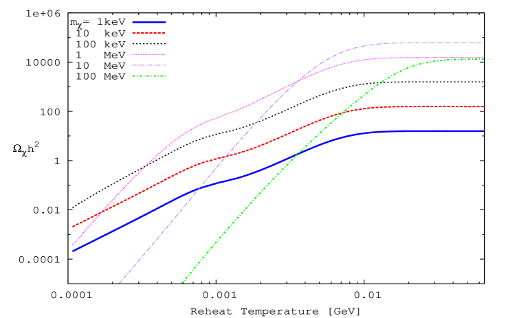
Figure 1: Relic abundance of the dark matter ($\chi$) as function of the reheat temperature for different values of $m_{\chi}$, in the presence of a decaying field $\phi$. The region below the reheat temperature 1 MeV is not of physical importance (kept just for the demonstrative purpose to show the variation), as it would be inconsistent with the Big Bang nucleosynthesis bound.

The behavior of $X$ can be roughly understood by considering Eq. (11), while the $\phi$-field is dominant (during reheating). Assuming that $\chi$ particles do not reach thermal equilibrium before the reheat temperature $T_{RH}$ is reached (${\it{i.e.}}X\ll X_{eq}$), Eq. (11) can be written as

$$\frac{dX}{dA}=CA^{-5/2}\langle\sigma_{\chi}v\rangle X_{eq}^{2},$$ (15)

where $C=\sqrt{\frac{3}{\Phi_{I}}}M_{P}T_{RH}$. Note that in this case $X$ (and hence the final relic abundance $\Omega_{\chi}h^{2}$) is proportional to $\langle\sigma_{\chi}v\rangle$ instead of the standard inverse dependence. The dependence on reheat temperature is also important to notice.

The results are depicted in Fig. 1, where the final contribution of dark matter particles to the mass density as a function of reheat temperature is plotted for different masses of the DM particle. These were obtained numerically (keeping all the terms in the set of Boltzmann equations) where the cross section is characterized by standard Fermi coupling (with cross section largely following Eq. (3); cf. Fig. 3). The number of relativistic degrees of freedom is approximated as a step function of temperature. We start with $g_{*}=2$ and when the temperature increases (or eventually decreases), as the calculation proceeds, $g_{*}$ is accordingly modified. Due to the discontinuity, the calculation is stopped and started with the new value of $T$, keeping other parameters constant. For most of the parameter range discussed here the equations are stiff and require an implicit scheme; we use a backward differentiation method (e.g., NR ), with relative tolerance $10^{-8}$ per time step. The integration is stopped once the comoving density $X$ converges to a constant asymptotic value with the same relative precision as the integration itself, provided reheating is complete (that is when $\phi$ becomes vanishingly small) and all variations in $g_{*}$ have ceased. In this case the present number density of particles is given by

$$n_{\chi}=\frac{X}{a_{c}^{3}}~{}\frac{a_{c}^{3}}{a_{o}^{3}}=\frac{X}{a_{c}^{3}}~{}\frac{T_{0}^{3}}{T_{c}^{3}},$$ (16)

where $T_{0}$ is the current CMB temperature, $T_{c}$ is the temperature at $X$ convergence (during the radiation era) and $a_{c}$ is the corresponding scale factor, given by $a_{c}=a_{I}A_{c}=A_{c}/T_{RH}$. The mass density is $\rho_{\chi}=m_{\chi}n_{\chi}$ and the contribution to the critical density is $\Omega_{\chi}=\rho_{\chi}/\rho_{\rm crit}$, with $\rho_{\rm crit}=3H_{0}^{2}/8\pi G$, so that $\Omega_{\chi}h^{2}=\frac{8\pi G\rho_{\chi}}{3}(\frac{h}{H_{0}})^{2}$. Here the scaled Hubble parameter, $h$, is defined through the Hubble constant at the present epoch, $H_{0}$, by $H_{0}=100h$ km $s^{-1}$ Mpc^-1.

In the cases considered in this section the DM particle production mechanism is thermal, since the $\phi$-field does not decay into WDM. However that does not necessarily imply that the particle has to reach chemical equilibrium, as will become clear from the following discussion. We divide the discussion into two parts. I. Region through which 1  ${\rm{keV}}\leq m_{\chi}<1~{}{\rm{MeV}}$: First note that the physically relevant region in this case corresponds to $m_{\chi}<T_{RH}$ when $T_{RH}>1$ MeV (to satisfy the Big Bang nucleosynthesis bounds). The curves in Fig. 1 can then be explained following the analytical result obtained in GKR . As found in GKR , $\Omega_{\chi}h^{2}$ is proportional to $T_{\rm RH}^{3}/g^{3/2}_{*}(T_{\rm RH})$ once the thermally averaged cross-section in Eq. (3) is considered, with $g_{*}(T_{\rm RH})$ referring to the number of relativistic degrees of freedom at reheating. Deviations from pure power law in our numerical calculations reflect the detailed evolution of $g_{*}$ as the full equations are integrated for different reheat temperatures. The rising sections of the curves correspond to the production of relativistic particles that do not reach chemical equilibrium. The dependence of $\Omega_{\chi}h^{2}$ on $T_{RH}$ flattens for higher range of $T_{RH}$. This is due to the fact that, as the reheat temperature is increased the DM particles come closer and closer to attaining chemical equilibrium. In this regime of relatively large $T_{RH}$, one recovers the abundance estimates associated with the standard scenario, which are again seen to be unrealistically large unless the particle mass is reduced to the eV, or hot dark matter, range. The inferred abundances for WDM particle mass in the keV range can indeed be consistent with observations only for $T_{RH}$ so low as to be marginally compatible with constraints from Big Bang nucleosynthesis.

II. Region through which $1~{}{\rm{MeV}}\leq m_{\chi}\leq 100~{}{\rm{MeV}}$: In this case $m_{\chi}$ could either be larger or smaller than $T_{RH}$. For large particle masses relative to $T_{\rm RH}$, the bulk of particle production occurs while the DM particle in consideration is non-relativistic and the inferred densities are proportional to $T_{\rm RH}^{7}$ GKR . The curve again flattens off as chemical equilibrium is reached after reheating. The case of $m_{\chi}=1~{}{\rm MeV}$ is intermediate; particle production is predominately in the relativistic regime for large $T_{\rm RH}$ and non-relativistic for smaller $T_{RH}$, with a transition around $T_{\rm RH}\sim m_{\chi}=1~{}{\rm MeV}$. The asymptotic densities are in line with estimates inferred in the context of the standard scenario using the same form of the cross-section employed in drees , and are unrealistically large. Thus, from Fig. 1, we conclude that the DM relic densities are only compatible with observations for very low reheat temperatures which is barely consistent with Big Bang nucleosynthesis. Furthermore, this only happens when the particle mass is of order 10 MeV or larger.

Thus, in the context considered here, particle masses are constrained either in the keV range or below and for reheat temperatures marginally consistent with nucleosynthesis constraints, and in possible tension with Lyman-$\alpha$ constraints Viel:2006kd ; VielN , or in the range of 10 MeV or above, in which case they would not ameliorate problems connected with galaxy formation. Below, however, we will replace this Fermi coupling by a $B-L$ one. In that case, since the mediator would be a sufficiently heavy particle (the gauge boson of $B-L$), the corresponding cross section, $\langle\sigma v\rangle$, of $\chi$ will be suppressed. This would further suppress the relic density as it is proportional to $\langle\sigma v\rangle$ for the non-equilibrium production of $\chi$ during reheating. So in that case, we expect $\Omega_{\chi}h^{2}$ to enter within the allowed range by WMAP and PLANCK.

IV WDM in $B-L$ Extension of the SM with Inverse Seesaw

As advocated in the introduction, one of the most attractive mechanisms that can naturally accommodate small neutrino masses with TeV scale right-handed neutrinos is what is known as the “Inverse Seesaw Mechanism”. This class of models predicts the following two types of neutrinos, besides the SM-like light neutrinos: $(i)$ Heavy (TeV) neutrinos, which are quite accessible and have interesting phenomenological implications; $(ii)$ Sterile light (keV) neutrinos, which has zero mixing with active neutrinos.

In this section we first show how the inverse seesaw mechanism can be naturally embedded in a low scale gauged $U(1)_{B-L}$ extension of the standard model. We also argue that it provides a natural candidate for WDM. The $B-L$ extension of the SM is based on the gauge group: $SU(3)_{C}\times SU(2)_{L}\times U(1)_{Y}\times U(1)_{B-L}$ Khalil:2006yi ; b-l ; Khalil:2010iu . The standard model is characterized by global $U(1)_{B-L}$ symmetry. If this symmetry is locally gauged, then the existence of three SM singlet fermions (the right-handed neutrinos) is a quite natural assumption to make in order to cancel the associated anomaly, which is a necessary condition for the consistency of the model. The extra $U(1)_{B-L}$ is spontaneously broken by a SM singlet scalar $\eta$ with $B-L$ charge $=-1$ Khalil:2010iu . The model therefore naturally predicts one extra neutral gauge boson $Z^{\prime}$ corresponding to $B-L$ gauge symmetry. In addition, three SM singlet fermions $\nu_{R_{i}}$ with $B-L$ charge $=-1$ are introduced for the consistency of the model. Finally, three SM pairs of singlet fermions $S_{1,2}$ with $B-L$ charge $=\mp 2$, respectively, are introduced to implement the inverse seesaw mechanism Khalil:2010iu . The $B-L$ quantum numbers of fermions and Higgs bosons of this model are summarized in Table 1. A discrete symmetry $Z_{4}$ is also considered in order to forbid several unwanted terms. The $Z_{4}$ charge assignment is included in Table  1.

Particle	$Q$	$u_{R}$	$d_{R}$	$L$	$e_{R}$	$\nu_{R}$	$h$	$\eta$	$S_{1}$	$S_{2}$
$Y_{B-L}$	$1/3$	$1/3$	$1/3$	$-1$	$-1$	$-1$	$0$	$-1$	$-2$	$+2$
$Z_{4}$	$1$	$1$	$1$	$-i$	$-i$	$-i$	$1$	$i$	$-1$	$1$

Table 1: $B-L$ quantum numbers and $Z_{4}$ charges of fermions and Higgs particles.

The Lagrangian of the leptonic sector in this model is given by Khalil:2010iu

$${\cal L}_{B-L} = -\frac{1}{4}F^{\prime}_{\mu\nu}F^{\prime\mu\nu}+i~{}\bar{L}D_{\mu}\gamma^{\mu}L+i~{}\bar{e}_{R}D_{\mu}\gamma^{\mu}e_{R}+i~{}\bar{\nu}_{R}D_{\mu}\gamma^{\mu}\nu_{R}$$ (17)

$$+ i~{}\bar{S}_{1}D_{\mu}\gamma^{\mu}S_{1}+i~{}\bar{S}_{2}D_{\mu}\gamma^{\mu}S_{2}+(D^{\mu}h)^{\dagger}D_{\mu}h+(D^{\mu}\eta)^{\dagger}D_{\mu}\eta-V(h,\eta)$$

$$- \Big{(}\lambda_{e}\bar{L}h\,e_{R}+\lambda_{\nu}\bar{L}\tilde{h}\nu_{R}+\lambda_{S}\bar{\nu}^{c}_{R}\eta S_{2}\Big{)}+h.c.,$$

where $F^{\prime}_{\mu\nu}$ is the field strength of the $U(1)_{B-L}$ and $h$ is the SM higgs field. Note that the $B-L$ symmetry allows a mixed kinetic term $F_{\mu\nu}F^{\prime\mu\nu}$. This term leads to a mixing between $Z$ and $Z^{\prime}$. However due to the stringent constraint from LEP II on $Z-Z^{\prime}$ mixing Carena:2004xs , one may neglect this term khalil-1105 . Therefore, after the $B-L$ and the EW symmetry breaking, through non-vanishing vacuum expectation values (VEVs) of $\eta$: $|\langle\eta\rangle|=v^{\prime}/\sqrt{2}$ and $h$: $|\langle h\rangle|=v/\sqrt{2}$, one finds that the neutrino Yukawa interaction terms lead to the following mass terms Khalil:2010iu :

$${\cal L}_{m}^{\nu}=m_{D}\bar{\nu}_{L}\nu_{R}+M_{N}\bar{\nu}^{c}_{R}S_{2}+h.c.,$$ (18)

where $m_{D}=\frac{1}{\sqrt{2}}\lambda_{\nu}v$ and $M_{N}=\frac{1}{\sqrt{2}}\lambda_{S}v^{\prime}$. Here $v^{\prime}$ is assumed to be of order TeV, which is consistent with the result of radiative $B-L$ symmetry breaking found in gauged $B-L$ model with supersymmetry Khalil:2007dr and $v=246$ GeV. Note that the spontaneous $B-L$ symmetry breaking leads to the following $Z^{\prime}$ gauge boson mass $M^{2}_{Z^{\prime}}=4g^{2}_{B-L}v^{\prime 2}$  ($g_{B-L}$ is the gauge coupling of $U(1)_{B-L}$). The experimental search for $Z^{\prime}$ LEP II Carena:2004xs implies that $M_{Z^{\prime}}/g_{B-L}>6\ {\rm TeV}$.

In addition one may generate very small Majorana masses for $S_{1,2}$ fermions through possible non-renormalizable terms like $\bar{S}^{c}_{1}{\eta^{\dagger}}^{4}S_{1}/M^{3}$ and $\bar{S}^{c}_{2}{\eta}^{4}S_{2}/M^{3}$. Note that the smallness of these masses are ensured by the choice of $Z_{4}$ charges of the fields involved. Therefore the Lagrangian of neutrino masses, in the flavor basis, is given by

$${\cal L}_{m}^{\nu}=\mu_{s}\bar{S}^{c}_{2}S_{2}+(m_{D}\bar{\nu}_{L}\nu_{R}+M_{N}\bar{\nu}^{c}_{R}S_{2}+h.c.),$$ (19)

where $\mu_{s}=\frac{v^{\prime 4}}{4M^{3}}\raise 1.29167pt\hbox{$\;<$\kern-7.5pt\raise-4.73611pt\hbox{$\sim\;$}}10^{-6}$ GeV. The choice of the discrete symmetry also forbids a possible large mixing term $mS_{1}S_{2}$ in the Lagrangian which could otherwise spoil the inverse seesaw structure. Therefore, the neutrino mass matrix can be written as ${\cal M}_{\nu}\bar{\psi}^{c}\psi$ with $\psi=(\nu_{L}^{c},\nu_{R},S_{2})$ where ${\cal M}_{\nu}$ is approximately given by,

$${\cal M}_{\nu}\simeq\left(\begin{array}[]{ccc}0&m_{D}&0\\ m^{T}_{D}&0&M_{N}\\ 0&M^{T}_{N}&\mu_{s}\\ \end{array}\right).$$ (23)

A few additional non-renormalizable terms can also be present. However, being small, their contributions are not incorporated in $M_{\nu}$ above. For example, terms like $LLhh{\eta^{\dagger}}^{2}/M^{3}$ and $\bar{L}hS_{2}{\eta}^{3}/M^{3}$ can contribute to 11 and 13 (or 31) entries of $M_{\nu}$ respectively. Nevertheless, the contribution of $LLhh{\eta^{\dagger}}^{2}/M^{3}$ is proportional to $\left(v/v^{\prime}\right)^{2}\mu_{s}$ and that of the other term is proportional to $\left(v/v^{\prime}\right)\mu_{s}$. Since $\left(v/v^{\prime}\right)\lesssim\cal{O}$ $\left(10^{-1}\right)$ and $\mu_{s}\sim 10^{-6}$ GeV only, these terms do not have much impact on the overall structure of $M_{\nu}$. Also there would be a small contribution to the right handed neutrino Majorana mass term, $m_{R}$, in the 22 entry of $M_{\nu}$, originating from ${\bar{\nu_{R}^{c}}}\nu_{R}{\eta^{\dagger}}^{2}/M$ that can not be prevented with the use of $Z_{4}$. However $m_{R}$ being small compared to the $m_{D}$ and $M_{N}$, its presence will not alter the light neutrino mass eigenvalues obtained from the above structure (Eq.(23)) to the leading order law .

The diagonalization of the mass matrix in Eq.(23) with nonzero $m_{R}$ leads to the following light and heavy neutrino masses Khalil:2010iu respectively in the leading order, under the consideration $m_{R},\mu_{s}\ll m_{D},M_{N}$   law :

$$m_{\nu_{l}} \simeq m_{D}M_{N}^{-1}\mu_{s}(M_{N}^{T})^{-1}m_{D}^{T},$$ (24)

$$m_{\nu_{H}}^{2} = m_{\nu_{H^{\prime}}}^{2}\simeq M_{N}^{2}+m_{D}^{2}.$$ (25)

Figure 2: Feynmann diagram for $S_{1}$ annihilation into light neutrinos, vis $Z^{\prime}$ gauge boson.

On the other hand, the second SM-singlet fermion, $S_{1}$, remains light with mass given by

$$m_{S_{1}}=\mu_{s}\simeq{\cal O}(1)~{}{\rm keV}.$$ (26)

It is important to note that the $S_{1}$ is a kind of sterile neutrino that has no mixing with active neutrinos. It only interacts with the gauge boson $Z^{\prime}$. Therefore, it is free from all constraints imposed on sterile neutrinos due to their mixing with the active neutrinos boyarsk2 . These constraints come mainly from the one loop decay channel into photon and active neutrino, which would produce a narrow line in the diffuse $\gamma$ and $X$ rays background radiation. This in turn implies that the mixing angle between sterile and active neutrinos is limited by boyarsk2

$$\theta\raise 1.29167pt\hbox{$\;<$\kern-7.5pt\raise-4.73611pt\hbox{$\sim\;$}}1.8\times 10^{-5}\left(\frac{\rm keV}{M_{\rm sterile}}\right)^{5}.$$

In contrast, the masses of our sterile neutrinos ($M_{\rm sterile}$) are not restricted to the keV range. Being odd under the $Z_{2}$, $S_{1}$ is a stable particle. So it is a quite natural candidate for warm dark matter. It annihilates through one channel only, into two light neutrinos mediated by $Z^{\prime}$, as shown in Fig. 2. The thermal averaged annihilation cross section of $S_{1}S_{1}\to\nu_{l}\nu_{l}$ is given by gelmini-gondolo-1009

$$\langle\sigma_{S_{1}}^{ann}v\rangle=\frac{\int_{0}^{\infty}dp~{}p^{2}W_{S_{1}S_{1}}(s)K_{1}(\frac{\sqrt{s}}{T})}{m_{S_{1}}^{4}T\left[K_{2}(\frac{m_{S_{1}}}{T})\right]^{2}},$$ (27)

where $W_{S_{1}S_{1}}$ is defined as the annihilation rate per unit volume and unit time seto through

$$W_{S_{1}S_{1}}(s)=\frac{1}{32\pi}\int\frac{d\cos\theta}{2}\sqrt{\frac{s-4m_{S_{1}}^{2}}{s}}|{\cal M}(S_{1}S_{1}\to\nu_{l}\nu_{l})|^{2},$$ (28)

with

$$\int\frac{d\cos\theta}{2}|{\cal M}(S_{1}S_{1}\to\nu_{l}\nu_{l})|^{2}=\frac{2}{3}\frac{|g_{B-L}^{2}q_{S_{1}}q_{\nu}|^{2}}{(s-M_{Z^{\prime}}^{2})^{2}+M_{Z^{\prime}}^{2}\Gamma_{Z^{\prime}}^{2}}(s-4m_{S_{1}}^{2})s.$$ (29)

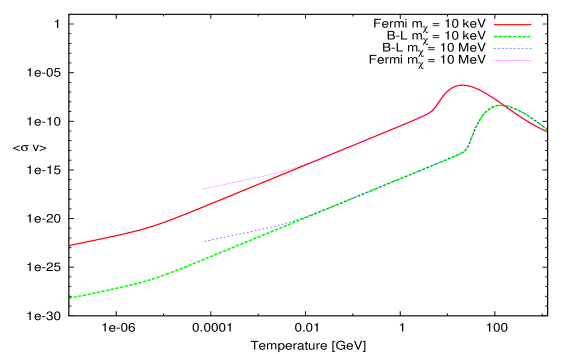
Figure 3: The thermally averaged annihilation cross section $\langle\sigma v\rangle$ (in GeV^-2) as function of the temperature (in GeV) when the WDM particle under consideration interacts through i) a Fermi coupling or ii) B-L coupling.

Here $s=4(m^{2}_{S_{1}}+p^{2})$ is the center of mass energy squared and $K_{1},K_{2}$ are the modified Bessel functions. $q_{S_{1}}=2$, $q_{\nu}=-1$ are the $B-L$ charges. The gauge boson $Z^{\prime}$ has the mass $M_{Z^{\prime}}$, would be of order ${\cal O}(100)$ GeV for $g_{B-L}={\cal O}(0.1)$, and its decay width is $\Gamma_{Z^{\prime}}$. In Fig. 3 we display the thermal averaged cross section $\langle\sigma^{ann}_{S_{1}}v\rangle$ as function of temperature $T$ for $m_{\chi}=10$ keV and 10 MeV with $M_{Z^{\prime}}=600$ GeV and $g_{B-L}=0.1$. In this plot, we also include the corresponding cross-section for a similar candidate of DM, when it has a standard Fermi coupling (with $M_{Z}=91.2~{}{\rm GeV}$, $\Gamma_{Z}=2.5~{}{\rm GeV}$ and $M_{W}=80.4~{}{\rm GeV}$), for illustration. As can be seen from Fig. 3, $\langle\sigma^{ann}v\rangle$ for the $B-L$ model is generally five to six orders of magnitude smaller than the cross section with Fermi coupling considered in the previous section, which is expected as the suppression factor turns out to be $\sim\left(g_{B-L}/g_{F}\right)^{4}\left(M_{Z}/M_{Z^{\prime}}\right)^{4}\sim 10^{-6}$   ($g_{F}$ is the gauge coupling constant in case of Fermi coupling). Note that this conclusion is largely independent of temperature and particle mass as well.

V WDM production during reheating in the $B-L$ model

In this section we study WDM production in the context of the $B-L$ model described above. In Section III it was impossible to consider the WDM particles as direct products of the $\phi$ field decay, without overproducing the DM content of the Universe. In the present case, we will show that this constraint can be relaxed. This is primarily because the cross section $\langle\sigma^{ann}v\rangle$ is different; we assign the WDM candidate with the $S_{1}$ field involved in inverse seesaw, and the related cross-section is approximately five or six orders of magnitude smaller compared to the case considered in section III with Fermi coupling. So we naturally expect that the dark matter abundances may radically differ from those inferred in section III. The prediction involves whether the dark matter particle reaches chemical equilibrium before reheating or not, whether the main particle production happens when the concerned particle is relativistic or not, and whether the field directly decays into the dark matter particle. We have tried to address these points in the rest of this section.

In order to realize WDM production through direct decay of the $\phi$-field, one should assume that the field has a strongly suppressed coupling with the WDM, $\chi$. Then $\Gamma_{\phi}$ describes the total decay width of $\phi$, inclusive of the decay into DM. We thus define the branching ratio of the $\phi$ field by $B_{\chi}$. The Boltzmann equations considered in section III are now replaced by the corresponding set Khalil:2002mu ,

$$\dot{\rho_{\phi}} = -3H\rho_{\phi}-\Gamma_{\phi}\rho_{\phi},$$ (30)

$$\dot{\rho_{R}} = -4H\rho_{R}+(1-B_{\chi})\Gamma_{\phi}\rho_{\phi}+\langle\sigma^{ann}_{\chi}v\rangle 2\langle E_{\chi}\rangle\left[(n_{\chi})^{2}-(n_{\chi}^{eq})^{2}\right],$$ (31)

$$\dot{n_{\chi}} = -3Hn_{\chi}+\frac{B_{\chi}}{m_{\chi}}\Gamma_{\phi}\rho_{\phi}-\langle\sigma^{ann}_{\chi}v\rangle\left[(n_{\chi})^{2}-(n_{\chi}^{eq})^{2}\right],$$ (32)

where $(1-B_{\chi})$ represents the decay into radiation. In terms of the previously defined normalized variables, the above set of equations can now be written as,

$$\frac{d\Phi}{dA} = -\left(\frac{\pi^{2}g_{*}}{30}\right)^{1/2}\frac{A^{1/2}\Phi}{\sqrt{\Phi+R/A+X\langle E_{\chi}\rangle/T_{RH}}},$$ (33)

$$\frac{dR}{dA} = \left(\frac{\pi^{2}g_{*}}{30}\right)^{1/2}\frac{\left(1-B_{\chi}\right)A^{3/2}\Phi}{\sqrt{\Phi+R/A+X\langle E_{\chi}\rangle/T_{RH}}}+\frac{{\sqrt{3}}M_{P}A^{-3/2}\langle\sigma^{ann}_{\chi}v\rangle 2\langle E_{\chi}\rangle\left[X^{2}-(X_{eq})^{2}\right]}{\sqrt{\Phi+R/A+X\langle E_{\chi}\rangle/T_{RH}}},$$ (34)

$$\frac{dX}{dA} = -3^{1/2}\frac{A^{-5/2}\langle\sigma_{\chi}v\rangle M_{P}T_{RH}}{\sqrt{\Phi+R/A+X\langle E_{\chi}\rangle/T_{RH}}}\left[X^{2}-(X_{eq})^{2}\right]+\frac{B_{\chi}}{m_{\chi}}\left(\frac{\pi^{2}g_{*}}{30}\right)^{1/2}\frac{A^{1/2}\Phi T_{RH}}{\sqrt{\Phi+R/A+X\langle E_{\chi}\rangle/T_{RH}}}.$$ (35)

We now begin to examine the relic densities of the predicted candidate $\chi\equiv S_{1}$ of the $B-L$ model using the above set of Boltzmann equations (33-35) and the annihilation cross section defined by Eq. (27). We plot the inferred density as a function of reheat temperature in Fig.4. Here we fix the mass of the WDM candidate as 1 keV. This is taken as a reference, as results are easily extrapolated for the mass range relevant to WDM; since (as in Fig. 1), for the mass range $\sim 1-100$ keV, the inferred abundances simply scale as $m_{\chi}$. Having fixed the mass, we consider the effect of different values of the $B_{\chi}$-parameter, which refers to the branching ratio of $\phi$-decay into $\chi\chi$. In addition, we include the case with $B_{\chi}=0$, which is analogous to what was considered in section III, with standard Fermi coupling. We have used the average WDM annihilation cross section as defined in Eq. (27), with $M_{Z^{\prime}}=600$ GeV and $g_{{}_{B-L}}=0.1$.

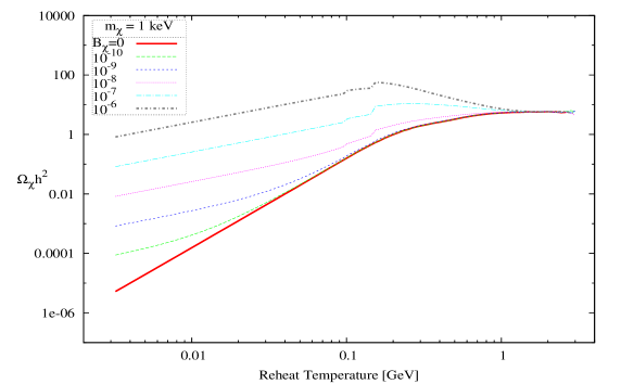
Figure 4: Thermal ($B_{\chi}=0)$ and non-thermal relic abundance for $B-L$ light sterile neutrino $S_{1}$ as function of the reheat temperature and different branching ratios of decay of the $\phi$ field into WDM particles.

First thing to note is that with $B_{\chi}\raise 1.29167pt\hbox{$\;<$\kern-7.5pt\raise-4.73611pt\hbox{$\sim\;$}}10^{-7}$ and low reheating, $T_{RH}\raise 1.29167pt\hbox{$\;<$\kern-7.5pt\raise-4.73611pt\hbox{$\sim\;$}}{\cal O}(0.01)$ GeV, one can easily account for the observed relic abundance and get $\Omega h^{2}\simeq 0.1$. While with $B_{\chi}=0$, a larger reheat temperature, $T_{RH}\sim{\cal O}(1)$ GeV is required. Since the annihilation cross section of $S_{1}$ is five orders of magnitudes smaller than the Fermi coupling cross section that has been considered in Section III, the relic density of $S_{1}$ WDM is also about five orders smaller than that used in Fig. 1; as the abundance, in this case, is proportional to $\langle\sigma v\rangle$ as can be seen from Eq. (36). This means, as is apparent from Fig. 4, that the relic abundance associated with WDM of mass $\sim 1$ keV can be consistent with the observational limits for $T_{RH}$ well above the Big Bang nucleosynthesis constraint: $T_{RH}\raise 1.29167pt\hbox{$\;>$\kern-7.5pt\raise-4.73611pt\hbox{$\sim\;$}}1$ MeV. Moreover, the whole mass range compatible with WDM can give rise to abundances consistent with empirical constraints on DM density and reheat temperature. This, as opposed to the case of standard Fermi coupling where the allowable range of relevant masses lay only in the keV range - rendering them in tension with lower mass limits inferred from Lyman-$\alpha$ observations - and with reheat temperatures marginally consistent with Big Bang nucleosynthesis.

When $B_{\chi}\neq 0$, the behavior of the curves in Fig. 4 is straightforward to explain in terms of non-thermal out of equilibrium production - in which case $\Omega_{\chi}h^{2}\propto T_{RH}$ - and non-thermal particle production while the coupling is strong enough to maintain chemical equilibrium, in which case $\Omega_{\chi}h^{2}\propto T_{RH}^{-1}$ Gelmini:2006pw . When production is dominated by the non-thermal channel, emanating from the decaying $\phi$-field, $\Omega_{\chi}h^{2}$ is proportional to $\propto B_{\chi}$, for a given reheat temperature. Bearing these scaling relations in mind (and recalling that $\Omega_{\chi}h^{2}\sim m_{\chi}$), the minimal case (of $m_{\chi}=1$ keV) described here can be used to put constraints on the branching ratio of $\phi$ field decay into WDM: for a given value of $m_{\chi}$ and $T_{RH}$, $B_{\chi}$ has to be below a certain (rather small) value to avoid over-production of WDM particles.

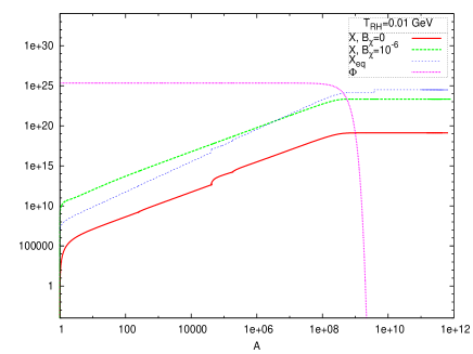
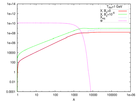
Figure 5: Evolution of the comoving abundance of a particle of mass 1 keV, as compared to the equilibrium abundance. Also shown is the evolution of the $\phi$ field in terms of $\Phi$.

We now take a more detailed look at the dynamics of the particle production mechanism. As we will see, the relevant processes crucially depend on the dynamics at reheating, because most of particle production occurs just before, or just after reheating is completed, that is at $T\sim T_{RH}$. In Fig. 5 we plot the evolution of the comoving densities $X$ and $X_{eq}$ and $\Phi$ (for the decaying scalar field $\phi$) as functions of the normalized scale factor $A=a/a_{I}$ (cf. Section III). Because $T_{RH}\gg m_{\chi}$, particles in kinetic equilibrium are relativistic. And since the relativistic equilibrium density $n_{eq}\sim T^{3}$, it follows that for relativistic particles $X_{eq}=n_{eq}a^{3}$ is constant during the radiation era (when $T\ll T_{RH}$), since in that case $T\sim 1/a\sim 1/A$. This explains the constant plateaus in the comoving densities for large $A$. However, as long as the $\phi$ field is dominant, $T\sim A^{-3/8}$ GKR , with the implication that $X_{eq}\sim A^{15/8}$, which is consistent with the initial behavior (for relatively small $A$) of the equilibrium density, as shown in Fig. 5.

The behavior of $X$ prior to reheating in the various cases can be largely understood by considering Eq. (35), while assuming the $\phi$-field is dominant. In this case it can be written as

$$\frac{dX}{dA}=-CA^{-5/2}\langle\sigma_{\chi}v\rangle(X^{2}-X_{eq}^{2})+DA^{1/2},$$ (36)

where $C=\sqrt{\frac{3}{\Phi_{I}}}M_{P}T_{RH}$ and $D=\frac{\pi B_{\chi}T_{RH}}{m_{\chi}}\sqrt{\frac{\Phi_{I}g_{*}}{30}}$ are constants (barring variations in $g_{*}$). In the case of relatively small reheat temperature (say $T_{RH}\sim 0.01$  GeV), the coupling $C$ is modest and the comoving density $X$ never reaches chemical equilibrium values; and so $X\ll X_{eq}$. In that case, and if $B_{\chi}=0$, Eq. (36) implies that $\frac{dX}{dA}\sim A^{-5/2}\langle\sigma_{\chi}v\rangle X_{eq}^{2}$, which scales as $A^{1/2}$ (since, from Fig. 3, $\langle\sigma_{\chi}v\rangle\sim T^{2}\sim A^{-3/4}$ in the relevant temperature range). This in turn implies $X\sim A^{3/2}$, which agrees with the corresponding curve shown on the left hand panel of Fig. 5. The same scaling is present if $B_{\chi}$ is non-zero and large enough; in this case the second term of Eq. (36) is dominant and $X\sim B_{\chi}A^{3/2}$; i.e., with the same scaling as the previous case but with different normalization.

For high $T_{\rm RH}\sim 1$ GeV, the coupling $C$ is strong enough; so that $X$ may quickly reach chemical equilibrium values when $B_{\chi}=0$; and so we find that (right hand panel of Fig. 5) $X\rightarrow X_{eq}$ for most of the evolution (with minor deviations at large $A$, when $X_{eq}$ is affected by temperature jumps due to variations in $g_{*}$ while the decoupled $X$ values remain constant after freeze out) . On the other hand if $B_{\chi}$ is large enough, we have $X\gg X_{eq}$ which leads to $\frac{dX}{dA}\approx-CA^{-5/2}\langle\sigma_{\chi}v\rangle X^{2}+DA^{1/2}$. The term $DA^{1/2}$ now represents a new ‘effective equilibrium’ value that $X$ tries to reach (so as to minimize $dX/dA$, as in the standard equilibrium situation when $X\rightarrow X_{eq}$); if this is the case one might expect that the $X$ evolution should obey

$$CA^{-5/2}\langle\sigma_{\chi}v\rangle X^{2}=DA^{1/2}.$$ (37)

Since, again, $\langle\sigma_{\chi}v\rangle\sim T^{2}\sim A^{-3/4}$; that means that the first term is proportional to $A^{-13/4}X^{2}$, which in turns implies that $X\sim A^{15/8}$, in this regime. This happens to scale the same way with $A$ as $X_{eq}$, but again with different normalization. When $A$ is large enough and $\Phi$ has decayed, $X$ converges to the equilibrium $X_{eq}$ before decoupling and freezing out.

Due to the shapes of the corresponding curves in Fig. 5 it is not obvious when ‘freeze out’ occurs. To get a better picture of the process we have also reproduced (Fig. 6) the logarithmic derivative $d\log X/d\log A=\frac{A}{X}\frac{dX}{dA}$ as a function of $A$. If freeze out happens before reheating is complete, $dX/dA$ will tend to zero even though $X_{eq}$ is still varying. In the terms of the scaled or normalized measure of the logarithmic derivative, freeze out can be defined as to occur when this is significantly smaller than one.

In Fig. 6 we plot the evolution of the logarithmic derivative $d\log X/d\log A$ versus $A$ for the cases with $B_{\chi}=0$ (the effect of the decaying field, represented by a non-zero $B_{\chi}$, clearly always freezes out when $\Phi\rightarrow 0$). We also add the evolution of the quantity $x=m_{X}/T$. The inflection point in $d\log X/d\log A$ evolution represents the end of the transition to the radiation dominated era (and this, as must be the case happens around $T_{RH}$, as represented by the horizontal lines). In the case of $T_{\rm RH}=0.01$  GeV, one finds that the freeze out occurs just around this transition, while for $T_{\rm RH}=1$  GeV, it occurs significantly later. In both cases freeze out occurs at quite small values of $x$, suggesting relativistic decoupling near $T_{RH}$.

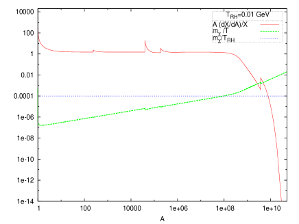
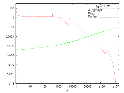
Figure 6: Evolution of the logarithmic derivative of the abundance of a particle of 1 keV, as compared to the equilibrium abundance for $B_{\chi}=0$ with $T_{RH}=0.01$ GeV (left panel) and $T_{RH}=1$ GeV (right panel). Also shown is the evolution of the quantity $x=m_{X}/T$.

We have thus far assumed that kinetic equilibrium is established even when the WDM particles are produced non-thermally through $\phi$-field decay; but given that our WDM particle interactions are strongly suppressed, this may not always be the case. In the absence of kinetic equilibrium, memory of the initial conditions of particle production is not lost, and so the WDM streaming length will depend on the initial kinetic energy imparted to the DM particles at production and on the epoch when this takes place. The streaming length will thus depend on the mass of the $\phi$-field and the reheat temperature, in addition to its dependence on the mass of $\chi$-particle.

An estimate of whether kinetic equilibrium is actually established chen , kawasaki can be obtained by applying the usual condition requiring that the scattering rate of the dark matter with other particles be larger than the expansion rate, $\Gamma^{\rm scatt}>H$; where $H$ is given by Eq.(13). The scattering rate is related to the scattering cross section ($\sigma_{s}$) and number density of scattering particles ($n$) as $\Gamma^{\rm scatt}=\sigma_{s}n$. Our proposed DM particles are expected to scatter off other particles (through the $t$-channel exchange of $Z^{\prime}$) with an estimate given by $\sigma_{s}\sim g^{4}_{B-L}\frac{E^{2}_{\chi}}{M^{2}_{Z^{\prime}}}$ (neglecting the mass of the $\chi$ particle), where $E_{\chi}$ is the energy associated with the $\chi$ particles. Considering $n\sim T^{3}$ and replacing $E_{\chi}$ by temperature $T$, we can write the condition for kinetic equilibrium at temperature $T=T_{RH}$ as:

$$T^{3}_{RH}M_{P}>\left(\frac{M_{Z^{\prime}}}{g_{B-L}}\right)^{4}.$$ (38)

With $g_{B-L}/M_{Z^{\prime}}\sim(6{\rm{TeV}})^{-1}$, this condition is satisfied for a reheat temperature $T_{RH}>0.1$ GeV. And it is sufficient that this condition be satisfied at reheating, following the $\phi$-field decay, for the WDM particles to attain kinetic equilibrium. Furthermore, one may expect that kinetic equilibrium is rapidly established as the reheat temperature increases above the limit just derived, since the ratio of the scattering rate to the expansion rate at reheating increases as $T_{RH}^{3}$; in this case, the streaming length will depend only on the mass of the $\chi$-particle; and as mentioned in the introduction, a generous WDM mass range is between 1 and 100 keV. However the range of reheat temperature we are interested in covers $T_{RH}$ between 0.01 GeV to 1 GeV. The steep temperature dependence should also ensure that significantly below the above critical temperature one can calculate the free streaming length while assuming that decay products of the $\phi$-field do not scatter at all (the intermediate case requires detailed calculation of the distribution function and requires a separate study). As mentioned above, since kinetic equilibrium is not established, one may expect the streaming length will depend on the mass of the $\phi$-field and the reheat temperature, as well as the mass of the $\chi$ particle – as indeed is found to be the case takahashi . For example, using the inequality in Eq.(15) of takahashi , and taking $m_{\phi}=1~{}{\rm TeV}$ and $T_{\rm RH}=0.01~{}{\rm GeV}$, we can estimate that our $\chi$ particles are WDM, in the sense satisfying the relevant Lyman alpha limit, if

$$\left(\frac{m_{\chi}}{\rm keV}\right)\raise 1.29167pt\hbox{$\;>$\kern-7.5pt\raise-4.73611pt\hbox{$\sim\;$}}2\times 10^{4}\epsilon,$$ (39)

where $\epsilon m_{\phi}/2$ is the energy imparted into a WDM particle by the decay of a $\phi$ particle. That is, for keV mass particles, the streaming length would be compatible with Lyman-$\alpha$ bounds Viel:2006kd ; VielN , if $\epsilon\sim 10^{-4}$.

Finally we note that the equations ($e.g.$ Eq. (32)) we have used to deduce the abundances are derived under the assumptions (a) the $\chi$ particles are created from and annihilate into particles that constitute a thermal bath, and (b) the $\chi$ particles themselves are in kinetic equilibrium. It is in this context that the thermally averaged cross section arises in those equations (instead of a cross section averaged over a general phase space distribution function). One may therefore ask if this formulation can still be used when assumption (b) is not satisfied, $i.e.$ when $T_{RH}<0.1$ GeV. To answer this question we note that, when deriving Eq.(32) from the full Boltzmann equations (involving the phase space distribution functions), assumption (b) is only necessary for deriving the terms involving $(n_{\chi})^{2}$; in contrast, terms with $(n_{\chi}^{\rm eq})^{2}$ are derived solely from assumption (a) Kolb+T . Now, these two terms in Eq.(32) translate into corresponding ones involving $X^{2}$ and $X_{\rm eq}^{2}$ in Eq. (36). Following the discussion subsequent to Eq.(36), it is apparent that, for low $T_{\rm RH}$ (and small $B_{\chi}$), our numerical results can be well understood by assuming $X\simeq 0$, as during relevant evolution $X\ll X_{\rm eq}$, which can be seen from Fig.5 (left hand panel), where the difference between $X_{\rm eq}^{2}$ and $X^{2}$ can be inferred to exceed ten orders of magnitude (for small $T_{\rm RH}$ and non-negligible $B_{\chi}$, $\chi$-particle production is dominated by direct $\Phi$-field decay, and therefore the manner in which the cross section is averaged over the phase space distribution makes little difference). Given this, it seems sufficient that the background bath be a thermal one for our abundance calculations to be valid to a good approximation at low $T_{\rm RH}$, since the term associated with assumption (b) should be small .

VI Conclusion

In the standard scenario, with high reheat temperature and equilibrium freeze out subsequent to reheating, the relic density of WDM with mass of order ${\cal O}(1)$ keV is unrealistically higher by several orders of magnitude than the observational limit. We have shown that, within low reheating scenario, the relic abundance of dark matter with mass of order keV or smaller or 10 MeV or larger, and annihilation cross section corresponding to standard Fermi coupling may be compatible with observations. However, keV WDM is in tension with Lyman-$\alpha$ and phase space density constraints due to its low mass and correspondingly large steaming length; the second case, of relatively high mass particles, is not relevant for solving problems related to the formation of galaxies, such as the overabundance of low mass DM halos or their apparent excessive concentrations. Indeed they are already non-relativistic at reheating and their steaming length will be too small to have any effect on the density fluctuation power spectrum as compared to standard CDM. Moreover, in both cases the required reheat temperatures are so low as to be marginally compatible with Big Bang nucleosynthesis constraints.

In contrast, due to a much smaller annihilation cross section, relic densities inferred in the context of the $B-L$ model are compatible with observations for the whole range of particle masses relevant to structure formation in the WDM scenario and with reheat temperatures compatible with Big Bang nucleosyntheis constraints. Our scenario also allows for the decay of the $\phi$ field into WDM particles during reheating. The results sensitively depend on the value of the branching ratio. Observational bounds on the possible relic abundance can be thus used to put upper limits on possible values of the branching ratios.

Acknowledgments: S.K. would like to acknowledge partial support by European Union FP7 ITN INVISIBLES (Marie Curie Actions, PITN-GA-2011-289442). A.S acknowledges the hospitality of CTP, Zewail City for Science and Technology, Cairo during a visit when this work was initiated. We thank the referee for careful reading of the manuscript and comments that helped improve the paper.

References

- (1) P. A. R. Ade et al. [Planck Collaboration], arXiv:1303.5076 [astro-ph.CO].
- (2) C. S. Frenk and S. D. M. White, Annalen Phys. 524, 507 (2012) [arXiv:1210.0544 [astro-ph.CO]].
- (3) B. Moore, S. Ghigna, F. Governato, G. Lake, T. R. Quinn, J. Stadel and P. Tozzi, Astrophys. J. 524, L19 (1999) [astro-ph/9907411].
- (4) A. A. Klypin, A. V. Kravtsov, O. Valenzuela and F. Prada, Astrophys. J. 522, 82 (1999) [astro-ph/9901240].
- (5) J. S. Bullock, A. V. Kravtsov and D. H. Weinberg, Astrophys. J. 539, 517 (2000) [astro-ph/0002214].
- (6) A. J. Benson, C. S. Frenk, C. G. Lacey, C. M. Baugh and S. Cole, Mon. Not. Roy. Astron. Soc. 333, 177 (2002) [astro-ph/0108218].
- (7) R. S. Somerville, Astrophys. J. 572, L23 (2002) [astro-ph/0107507].
- (8) T. Okamoto and C. S. Frenk, arXiv:0909.0262 [astro-ph.CO].
- (9) M. Wadepuhl and V. Springel, arXiv:1004.3217 [astro-ph.CO].
- (10) A. M. Brooks, M. Kuhlen, A. Zolotov and D. Hooper, Astrophys. J. 765, 22 (2013) [arXiv:1209.5394 [astro-ph.CO]].
- (11) H. Pagels and J. R. Primack, Phys. Rev. Lett. 48, 223 (1982); P. J. E. Peebles, Astrophys.J. 258, 415 (1982); J. R. Bond, A. S. Szalay and M. S. Turner, Phys. Rev. Lett. 48, 1636 (1982); K. A. Olive and M. S. Turner, Phys. Rev. D 25 (1982) 213.
- (12) S. Colombi, S. Dodelson and L. M. Widrow, Astrophys. J. 458, 1 (1996) [astro-ph/9505029].
- (13) J. M. Bardeen, J. R. Bond, N. Kaiser and A. S. Szalay, Astrophys. J. 304, 15 (1986).
- (14) P. Bode, J. P. Ostriker and N. Turok, Astrophys. J. 556, 93 (2001) [astro-ph/0010389].
- (15) M. Viel, J. Lesgourgues, M. G. Haehnelt, S. Matarrese and A. Riotto, Phys. Rev. D 71, 063534 (2005) [astro-ph/0501562].
- (16) A. Schneider, R. E. Smith, A. V. Maccio and B. Moore, Mon. Not. Roy. Astron. Soc. 424, 684 (2012) arXiv:1112.0330 [astro-ph.CO].
- (17) M. R. Lovell, V. Eke, C. S. Frenk, L. Gao, A. Jenkins, T. Theuns, J. Wang and D. M. White et al., Mon. Not. Roy. Astron. Soc. 420, 2318 (2012) [arXiv:1104.2929 [astro-ph.CO]].
- (18) S. Shao, L. Gao, T. Theuns and C. S. Frenk, arXiv:1209.5563 [astro-ph.CO].
- (19) A. Boyarsky, J. Lesgourgues, O. Ruchayskiy and M. Viel, Phys. Rev. Lett. 102, 201304 (2009) [arXiv:0812.3256 [hep-ph]].
- (20) A. Boyarsky, O. Ruchayskiy and M. Shaposhnikov, Ann. Rev. Nucl. Part. Sci. 59, 191 (2009) [arXiv:0901.0011 [hep-ph]].
- (21) M. Viel, J. Lesgourgues, M. G. Haehnelt, S. Matarrese and A. Riotto, Phys. Rev. Lett. 97, 071301 (2006) [astro-ph/0605706].
- (22) M. Viel, G. D. Becker, J. S. Bolton and M. G. Haehnelt, arXiv:1306.2314 [astro-ph.CO].
- (23) C. R. Watson, J. F. Beacom, H. Yuksel and T. P. Walker, Phys. Rev. D 74, 033009 (2006) [astro-ph/0605424].
- (24) R. E. Marshak and R. N. Mohapatra, Phys. Lett. B 91, 222 (1980).
- (25) R. N. Mohapatra and R. E. Marshak, Phys. Rev. Lett. 44, 1316 (1980) [Erratum-ibid. 44, 1643 (1980)].
- (26) S. Khalil, J. Phys. G 35, 055001 (2008)
- (27) Q. R. Ahmad et al. [SNO Collaboration], Phys. Rev. Lett. 89, 011301 (2002); S. N. Ahmed et al. [SNO Collaboration], Phys. Rev. Lett. 92, 181301 (2004); K. Eguchi et al. [KamLAND Collaboration], Phys. Rev. Lett. 90, 021802 (2003); M. H. Ahn et al. [K2K Collaboration], Phys. Rev. D 74, 072003 (2006); D. G. Michael et al. [MINOS Collaboration], Phys. Rev. Lett. 97, 191801 (2006); M. Apollonio et al. [CHOOZ Collaboration], Phys. Lett. B 466, 415 (1999); K. Abe et al. [T2K Collaboration], Phys. Rev. Lett. 107, 041801 (2011); P. Adamson et al. [MINOS Collaboration], Phys. Rev. Lett. 107, 181802 (2011); Y. Abe et al. [DOUBLE-CHOOZ Collaboration], Phys. Rev. Lett. 108, 131801 (2012); F. P. An et al. [DAYA-BAY Collaboration], Phys. Rev. Lett. 108, 171803 (2012); S. Nakayama [T2K Collaboration], J. Phys. Conf. Ser. 375, 042070 (2012).
- (28) S. Khalil, Phys. Rev. D 82, 077702 (2010)
- (29) G. Hinshaw et al. [WMAP Collaboration], arXiv:1212.5226 [astro-ph.CO].
- (30) M. Drees, M. Kakizaki and S. Kulkarni, Phys. Rev. D 80, 043505 (2009) [arXiv:0904.3046 [hep-ph]].
- (31) B. A. Bassett, S. Tsujikawa and D. Wands, Rev. Mod. Phys. 78, 537 (2006) [astro-ph/0507632].
- (32) G. F. Giudice, E. W. Kolb and A. Riotto, Phys. Rev. D 64 (2001) 023508 [hep-ph/0005123].
- (33) G. B. Gelmini and P. Gondolo, Phys. Rev. D 74, 023510 (2006) [hep-ph/0602230].
- (34) T. Moroi and L. Randall, Nucl. Phys. B 570, 455 (2000) [hep-ph/9906527].
- (35) D. J. H. Chung, E. W. Kolb and A. Riotto, Phys. Rev. D 60, 063504 (1999) [hep-ph/9809453].
- (36) C. Wetterich, Nucl. Phys. B 187, 343 (1981); M. Abbas and S. Khalil, JHEP 0804, 056 (2008); W. Emam and S. Khalil, Eur. Phys. J. C 55, 625 (2007); K. Huitu, S. Khalil, H. Okada and S. K. Rai, Phys. Rev. Lett. 101, 181802 (2008); L. Basso, A. Belyaev, S. Moretti and C. H. Shepherd-Themistocleous, Phys. Rev. D 80, 055030 (2009); L. Basso, A. Belyaev, S. Moretti, G. M. Pruna and C. H. Shepherd-Themistocleous, PoS EPS-HEP2009, 242 (2009); L. Basso, S. Moretti and G. M. Pruna, Phys. Rev. D 83, 055014 (2011); L. Basso, A. Belyaev, S. Moretti and G. M. Pruna, J. Phys. Conf. Ser. 259, 012062 (2010); S. K. Majee and N. Sahu, Phys. Rev. D 82, 053007 (2010); T. Li and W. Chao, Nucl. Phys. B 843, 396 (2011); P. Fileviez Perez, T. Han and T. Li, Phys. Rev. D 80, 073015 (2009);
- (37) M. Carena, A. Daleo, B. A. Dobrescu and T. M. P. Tait, Phys. Rev. D 70, 093009 (2004); T. Appelquist, B. A. Dobrescu and A. R. Hopper, Phys. Rev. D 68, 035012 (2003).
- (38) W. Abdallah, A. Awad, S. Khalil and H. Okada, Eur. Phys. J. C 72, 2108 (2012) [arXiv:1105.1047 [hep-ph]].
- (39) S. Khalil and A. Masiero, Phys. Lett. B 665, 374 (2008);
- (40) S. S. C. Law and K. L. McDonald, Phys. Rev. D 87, no. 11, 113003 (2013) [arXiv:1303.4887 [hep-ph]]; Y. -L. Zhou, Phys. Rev. D 86, 093011 (2012) [arXiv:1205.2303 [hep-ph]].
- (41) G. Gelmini and P. Gondolo, In *Bertone, G. (ed.): Particle dark matter* 121-141 [arXiv:1009.3690 [astro-ph.CO]].
- (42) S. Khalil and O. Seto, JCAP 0810, 024 (2008) [arXiv:0804.0336 [hep-ph]].
- (43) S. Khalil, C. Munoz and E. Torrente-Lujan, New J. Phys. 4, 27 (2002) [hep-ph/0202139].
- (44) W. H. Press, B. R. Flannery, S. A. Teukolsky and W. T. Vetterling, Numerical Recipes in FORTRAN (Cambridge University Press 1989).
- (45) X. -l. Chen, M. Kamionkowski and X. -m. Zhang, Phys. Rev. D 64, 021302 (2001) [astro-ph/0103452].
- (46) K. Harigaya, M. Kawasaki, K. Mukaida and M. Yamada, arXiv:1402.2846 [hep-ph].
- (47) F. Takahashi, Phys. Lett. B 660, 100 (2008) [arXiv:0705.0579 [hep-ph]].
- (48) E. W. Kolb and M. S. Turner, The Early Universe (Westview Press 1994).