Quantum noise eater for a single photonic qubit

Abstract

We propose a quantum noise eater for a single qubit and experimentally verify its performance for recovery of a superposition carried by a dual-rail photonic qubit. We consider a case when only one of the rails (e.g., one of interferometric arms) is vulnerable to noise. A coherent but randomly arriving photon penetrating into this single rail causes a change of its state, which results in an error in a subsequent quantum information processing. We theoretically prove and experimentally demonstrate a conditional full recovery of the superposition by this quantum noise eater.

1 Introduction

A success of any application of quantum physics strongly depends on accessibility and quality of quantum resources. Quantum bit (qubit), being quantum analog of classical bit, is a fundamental but fragile element of quantum information [1]. It is the simplest quantum system with the smallest Hilbert space of quantum states consisting all possible superpositions of two basis states. Many physical systems have been experimentally proved to exhibit such superpositions applicable for quantum information processing [2, 3, 4, 5, 6, 7, 8, 9, 10, 11, 12, 13, 14]. However, a quantum superposition can simply be lost by noise driving qubit to a mixture of basis states [1, 15]. The noise can exhibit many different characteristics depending on a coupling of qubit to a noisy environment and also on a state of the noisy environment. Many methods of protection of single qubit against the noise have been proposed [16, 17, 18]. Typically, they are designed for a specific type of noise influencing well defined Hilbert space of qubit.

However, single-qubit superposition can be also destroyed by very destructive random coherent noise, that transforms a qubit to a system with a higher dimension. The simplest example is a qubit represented by a (bosonic) particle which can be coherently mixed with another indistinguishable particle [19, 20]. It is an elementary case of a more complex coherent continuous-variable noise [21], where the number of such particles coming from the environment fluctuates. In past, many techniques based on quantum feedback [22] have been experimentally verified to reduce this destructive continuous noise. A technique commonly used in such a case is a noise eater [25], which is able to detect intensity of a small part of the coherent signal mixed with noise and use adjustable feed-back loop to control the laser (or modulate light) to reduce that noise at a cost of lower output optical power. Recently, different techniques based on multiple copies of noisy coherent states [23] and measurement of noise from an environment [24] have been also tested. Also probabilistic version of the noise eater reducing non-Gaussian intensity noise imposed on the coherent states have been verified [26]. However, a single particle “penetrating to a qubit” can be even more destructive. If the signal and noise particles are principally distinguishable but technically indistinguishable, quality of a qubit is substantially damaged [27]. But even if the particles are principally indistinguishable and the superposition just expands coherently to a higher dimensional state, it causes problems because many operations are designed specifically for qubits, they expect only 2D Hilbert space.

In this paper, we propose and perform a proof-of-principle experimental test of the simplest coherent noise eater technique for a qubit carrying quantum superposition. We study the simplest case when, during an elementary noise impact, the dual-rail photonic qubit is influenced by a single indistinguishable noise photon in only one (known) rail. Similarly to the noise eater technique for laser light, a partial detection of number of photons in optical beam is exploited, however with single photon resolution. Moreover, differently to that technique, measured information is used to herald only the cases when at most one photon remains in the setup. To test quality of the resulting qubit, we evaluate visibility of interference in a subsequent Hadamard gate acting on that qubit. It appears that the proposed noise eater is able to recover visibility of interference up to unity.

2 Coherent noise eater for a dual-rail qubit

The noise eater technique can be based, e.g., on photon-number measurement which conclusively detects exactly one photon in the propagating beam and simultaneously leaves desired superposition unchanged. If one finds more than one photon in the beam he/she rejects that case and does not use the state for further applications. Situations heralded by this procedure correspond to true qubits carried by individual photons. Therefore no error from multi-photon contribution can appear. If the noise photon is fully indistinguishable from the signal photon, the noise effect is caused purely by an extension of the total state of the system to a higher dimensional single-mode Hilbert space. Such noise can be completely eliminated by the ideal noise eater. It is an example of quantum coherent nondestructive filtering, which requires photon number resolution. When the signal and noise photons are partially distinguishable (due to the different states of non-informational degrees of freedom) the situation can be conditionally converted to the previously described ideal case by classical filtering in front of the noise eater. Unfortunately, the required ideal nondestructive photon-number resolving detectors are currently not feasible. However, we have devised an alternative implementation which still works well for our particular situation but makes do with standard photonic technology.

Recently, a quantum relay has been used to detect whether a photon is present in a beam or not [28, 29]. It allows to conditionally avoid an impact of a noise photon in a subsequent quantum channel. However, our situation is rather opposite, since the noisy photon could already affect the qubit. Therefore we need to end up with one photon exactly. In continuous variables, coherent state filtration has been experimentally tested to avoid non-Gaussian noise [26], however, it heralds on higher photon numbers rather than on exactly a single photon state. On the other hand, in our proof-of-principle experiment we know that only a single noise photon can enter the system. So we can substitute nondestructive photon-number measurement followed by rejection of any multi-photon contributions by the subtraction of a single photon after the noise impact. The photon is subtracted using a linear optical device that spatially separates two incoming photons with nonzero probability and detects one of them afterwards. If a photon is subtracted then only one photon remains in the dual-rail qubit. When the signal and noise photons are fully indistinguishable, this simplified linear-optical version of the noise eater technique can reach the perfect recovery of qubit superposition, irrespective of the probability of the noise impact.

A single photon being in a superposition of two spatial rails can be used to experimentally demonstrate this prospective method. Two basis states $|0,1\rangle_{AB}$ and $|1,0\rangle_{AB}$ represent a photon being either in the rail A or B. Equatorial states in the form of $(|0,1\rangle_{AB}+\exp(i\varphi)|1,0\rangle_{AB})/\sqrt{2}$ carry quantum information encoded to balanced superpositions of the basis states. A unitary Hadamard gate is represented by symmetrical coupling between the both rails. Ideally, it builds superposition $|+\rangle_{AB}=(|0,1\rangle_{AB}+|1,0\rangle_{AB})/\sqrt{2}$ from state $|1,0\rangle_{AB}$. The single-qubit Hadamard gate can be simply implemented by a balanced beam splitter transformation $U_{H}=\left(\frac{1}{\sqrt{2}}\right)^{n_{A}}\exp\left(-\frac{a_{B}^{\dagger}a_{A}}{\sqrt{2}}\right)\exp\left(\frac{a_{A}^{\dagger}a_{B}}{\sqrt{2}}\right)\left(\frac{1}{\sqrt{2}}\right)^{-n_{B}}$ working on complete Hilbert spaces of two modes $A$ and $B$ ($n_{A},n_{B}$ are photon-number operators). To test the quality of preparation of this superposition, we consider another subsequent Hadamard gate that should reverse the superposition states $|+\rangle_{AB}$ back to a complementary-basis state $|1,0\rangle_{AB}=(|+\rangle_{AB}+|-\rangle_{AB})/\sqrt{2}$ .

If the noise photon coming from the environment is indistinguishable from the signal photon, a coherent superposition $(\sqrt{2}|0,2\rangle_{AB}+|1,1\rangle_{AB})/\sqrt{3}$ arises in a larger Hilbert space of the same modes. This superposition can still perfectly carry any phase information imposed, for example, by $U_{PS}=\exp(i\phi n_{A})$. On the other hand, both the state $|0,2\rangle_{AB}$ and $|1,1\rangle_{AB}$ generates unavoidable errors in our implementation of the Hadamard gate $U_{H}$ due to the presence of another photon. However, by subtraction of a single photon from mode B we conditionally reach state $(2|0,1\rangle_{AB}+|1,0\rangle_{AB})/\sqrt{5}$ which can be balanced by simple amplitude damping back to the original superposition $|+\rangle_{AB}$. It clearly demonstrates that by combination of classical filtration and quantum noise eater technique, the original superposition state of a qubit influenced by coherent single-photon noise can be fully restored.

3 Theoretical description of experimental test

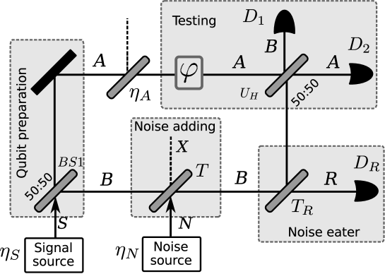
Figure 1: Set-up for proof-of-principle test of coherent noise quantum eater for dual-rail qubit. $T$ is intensity transmission of the beam splitter (the $T$ is the transmission ratio of the photons coming from the left to right), $T_{R}$ is the intensity transmission of the beam splitter (the $T_{R}$ is the transmission ratio of the photons coming from the left to right), $D_{i}$ are detectors, $\varphi$ is a phase shifter, $\eta_{A}$ is the intensity transmission of the beam splitter (attenuator), signal resp. noise source generate single photon with probability $\eta_{S}$ resp. $\eta_{N}$.

A detailed scheme of the proof-of-principle test of the proposed single-photon noise eater is depicted in figure 1. The scheme is divided into stages that help to visualize the whole protocol. Signal photon enters to the qubit preparation stage from the source of photons with probability $\eta_{S}$. Then a beam splitter BS1 splits the photon equally into both rails, where the resulting equatorial dual-rail qubit state is created $\frac{1}{\sqrt{2}}(|0,1\rangle+|1,0\rangle)$ During the noise adding stage, coherent noise photon is penetrating into the qubit from single-photon source with probability $\eta_{N}$ by a beam splitter with intensity transmission $T$ (the $T$ is the transmission ratio of the signal coming from the left to right in Fig. 1).

To evaluate impact of the single-photon noise on the qubit without any action of the noise eater, we set $T_{R}=0$. Then we close the interferometric setup by placing another Hadamard gate $U_{H}$ that merges both rails. We can directly quantify the quality of a qubit after the addition of noise by visibility. To evaluate it we vary phase $\varphi$ in the testing stage and measure the probability $P(\varphi)$ of a count at the one output port of the Hadamard gate. Visibility is defined by $V=\frac{P_{\max}-P_{\min}}{P_{\max}+P_{\min}}$, where $P_{\max}=\max_{\varphi}P(\varphi)$ ($P_{\min}=\min_{\varphi}P(\varphi)$) is maximum (minimum) of $P(\varphi)$ over $\varphi$. To maximize visibility, we use another amplitude damping operations on qubit represented by an attenuator with intensity transmission $\eta_{A}$ (transmission ratio of the signal coming from the left to right in Fig. 1) placed in the rail $A$.

The probability to detect at least one photon at detector D₁ (or D₂) with detector efficiency $\eta_{D}$ will be sum of three independent terms coming from different states going through the MZ interferometer. The first state $|\psi_{1}\rangle=\sqrt{1-\eta_{S}}\sqrt{\eta_{N}}|01\rangle_{SN}$ represents the situation of one photon in noise mode and no photon in signal mode, second state $|\psi_{2}\rangle=\sqrt{\eta_{S}}\sqrt{1-\eta_{N}}|10\rangle_{SN}$ represents the situation of one photon in signal mode and no photon in noise mode and the third state $|\psi_{3}\rangle=\sqrt{\eta_{S}}\sqrt{\eta_{N}}|11\rangle_{SN}$ represents the situation of one photon in signal mode and one photon in noise mode.

In the following we show steps of calculation for getting output states $|\psi_{i}^{\prime}\rangle$ from the input states $|\psi_{i}\rangle$. The quantum modes used in the calculations are shown in the Fig. 1. The symbols over the right arrows represent the transformations used to obtain next step, e.g. $BS(T)$ means beam splitter $T$ with intensity transition $T$, $PS(\varphi)$ is a phase shifter with phase shift $\varphi$.

$$|\psi_{1}\rangle\xrightarrow{BS(T)}\sqrt{1-\eta_{S}}\sqrt{\eta_{N}}(\sqrt{T}|01\rangle_{BX}+i\sqrt{1-T}|10\rangle_{BX}\xrightarrow{BS(1/2)}\\ |\psi_{1}^{\prime}\rangle=\sqrt{1-\eta_{S}}\sqrt{\eta_{N}}(\sqrt{T}|001\rangle_{ABX}+i\sqrt{\frac{(1-T)}{2}}(i|100\rangle_{ABX}+|010\rangle_{ABX})$$ (1)

The probability to detect a photon in mode $B$ with detector efficiency $\eta_{D}$ reads

$$P_{1}=\Tr(|1\rangle_{B}\langle 1|\psi_{1}^{\prime}\rangle\langle\psi_{1}^{\prime}|)=\frac{\eta_{D}\eta_{N}(1-\eta_{S})(1-T)}{2}$$

$$|\psi_{2}\rangle\xrightarrow{BS(1/2)}\frac{\sqrt{\eta_{S}}\sqrt{1-\eta_{N}}}{\sqrt{2}}(|10\rangle_{AB}+i|01\rangle_{BX})\xrightarrow{BS(\eta_{A}),\;BS(T),\;PS(\varphi)}\\ \frac{\sqrt{\eta_{S}}\sqrt{1-\eta_{N}}}{\sqrt{2}}(\sqrt{\eta_{A}}\exp{(i\varphi)}|100\rangle_{ABX}+i|0\rangle_{A}(\sqrt{T}|10\rangle_{BX}+\sqrt{1-T}|01\rangle_{BX})\xrightarrow{BS(1/2)}\\ |\psi_{2}^{\prime}\rangle=\frac{\sqrt{\eta_{S}}\sqrt{1-\eta_{N}}}{\sqrt{2}}(\exp{(i\varphi)}\frac{\sqrt{\eta_{A}}}{\sqrt{2}}(|10\rangle_{AB}+i|01\rangle_{AB})|0\rangle_{X}+\\ +\frac{i\sqrt{T}}{\sqrt{2}}(|01\rangle_{AB}+i|10\rangle_{AB})|0\rangle_{X}+i\sqrt{1-T}|001\rangle_{ABX})$$ (2)

The probability to detect a photon in mode $B$ with detector efficiency $\eta_{D}$ reads

$$P_{2}=\Tr(|1\rangle_{B}\langle 1|\psi_{2}^{\prime}\rangle\langle\psi_{2}^{\prime}|)=\frac{\eta_{D}\eta_{S}(1-\eta_{N})(\eta_{A}+T-2\sqrt{\eta_{A}T}\cos\varphi)}{4}$$

$$|\psi_{3}\rangle\xrightarrow{BS(1/2),\;BS(\eta_{A}),\;PS(\varphi)}\frac{\sqrt{\eta_{S}\eta_{N}}}{\sqrt{2}}(i|011\rangle_{ABN}+\exp{(i\varphi)}\sqrt{\eta_{A}}|101\rangle_{ABN})\xrightarrow{BS(T)}\\ \frac{\sqrt{\eta_{S}\eta_{N}}}{\sqrt{2}}(i|0\rangle_{A}(i\sqrt{2T(1-T)}|20\rangle_{BX}+i\sqrt{2T(1-T)}|02\rangle_{BX}+(2T-1)|11\rangle_{BX})+\\ +\exp{(i\varphi)}\sqrt{\eta_{A}}|1\rangle_{A}(i\sqrt{1-T}|10\rangle_{BX}+\sqrt{T}|01\rangle_{BX}))\xrightarrow{BS(1/2)}|\psi_{3}^{\prime}\rangle=\\ \frac{\sqrt{\eta_{S}\eta_{N}}}{\sqrt{2}}(-\sqrt{2T(1-T)}(\frac{1}{2}|02\rangle_{AB}-\frac{1}{2}|20\rangle_{AB}+\frac{i}{\sqrt{2}}|11\rangle_{AB})+\frac{i(2T-1)}{\sqrt{2}}(|01\rangle_{AB}+|10\rangle_{AB})-\\ -\exp(i\varphi)\frac{\sqrt{\eta_{A}(1-T)}}{\sqrt{2}}(|20\rangle_{AB}+|02\rangle_{AB})+\exp(i\varphi)\frac{\sqrt{\eta_{A}T}}{\sqrt{2}}(i|01\rangle_{AB}+|10\rangle_{AB})$$ (3)

The probability to detect at least one photon (one or two) in mode $B$ with detector efficiency $\eta_{D}$ reads

$$P_{3}=\Tr((|1\rangle_{B}\langle 1|+|2\rangle_{B}\langle 2|)|\psi_{3}^{\prime}\rangle\langle\psi_{3}^{\prime}|)=\\ \frac{1}{4}\left(\eta_{D}\eta_{S}\eta_{N}(\eta_{A}(1-\eta_{D})+2+T+\eta_{D}T(T-1+\eta_{A})+(\eta_{D}(1-T)-1)2\sqrt{\eta_{A}T}\cos(\varphi))\right)$$ (4)

Adding the three probabilities together gives us

$$P=P_{1}+P_{2}+P_{3}=\frac{\eta_{D}}{4}\left(W_{1}+W_{2}\cos\varphi\right),$$ (5)

where $W_{1}=2\,\eta_{{N}}+\eta_{{S}}\eta_{{A}}+\eta_{{S}}\eta_{{N}}T\eta_{D}\eta_{{A}}-2\,\eta_{{N}}T-\eta_{{S}}\eta_{{N}}\eta_{D}T+\eta_{{S}}T-\eta_{{S}}\eta_{{N}}\eta_{D}\eta_{{A}}+\eta_{{S}}\eta_{{N}}{T}^{2}\eta_{D}$ and $W_{2}=2\,\eta_{{S}}\eta_{{N}}\eta_{D}\sqrt{T}\sqrt{\eta_{{A}}}-2\,\eta_{{S}}\eta_{{N}}{T}^{3/2}\eta_{D}\sqrt{\eta_{{A}}}-2\,\eta_{{S}}\sqrt{T}\sqrt{\eta_{{A}}}$ determine a depth of modulation of the interference fringe. The corresponding visibility of interference for balanced optical paths $\eta_{A}=T$ reads

$$V=\frac{W_{2}}{W_{1}}=\frac{\eta_{S}T(\eta_{N}T\eta_{D}-\eta_{N}\eta_{D}+1)}{\eta_{S}\eta_{N}\eta_{D}T(T-1)+\eta_{S}T+\eta_{N}(1-T)}.$$ (6)

It can be further simplified, for equal input signal and noise losses $\eta_{S}=\eta_{N}$ and for detector efficiency $\eta_{D}=0.5$ used in the experiment, to the following form

$$V=\frac{2T+\eta_{S}T(T-1)}{2+\eta_{S}T(T-1)}.$$ (7)

For typical $\eta_{S}=\eta_{N}\ll 1$, the reduced visibility simply approaches

$$V\approx T.$$ (8)

Irrespective of full coherence between the signal and noise photons, visibility is directly proportional to the probability that signal photon arrives to a detector. The reduction comes simply from the fact that noise photon, although fully coherent does not carry information about testing phase $\varphi$. Either the signal or noise photon randomly arrives to the Hadamard gate and compensation by $\eta_{A}$ is actually redundant. The prepared state remains dominantly in the original 2D Hilbert space, since contribution of the bunching is negligible. For $\eta_{S}=\eta_{N}\ll 1$, we get the same visibility $V\approx T$ also for noisy photon being fully distinguishable. These two cases are therefore problematically distinguishable if only the reduction of visibility is analyzed (see figure 3 for both plots).

For lower transmission $T$, the reduction of visibility is really substantial. To increase the visibility, we use an elementary noise eater consisting of beam splitter with intensity transmission $T_{R}$ (the $T_{R}$ is the transmission ratio of the photons coming from the left to the right in Fig. 1) and single photon detector $D_{R}$ right after the coupling of noise photon. We optimize $\eta_{A}$ and $T_{R}$ and measure the visibility at the detector $D_{1}$ conditioned now by detection of a photon at detector $D_{R}$. We exploit the very rare but still present bunching effect, when the signal and noise photons become indistinguishable. The conditional probability of photon detection at $D_{1}$ when one photon has already been detected at $D_{R}$ can be calculated using just the state $|\psi_{3}\rangle$ since the other two single photon states $|\psi_{1}\rangle$ and $|\psi_{2}\rangle$ would not contribute to coincidence detection.

We again show the steps of calculations to obtain an output state $|\psi_{c}\rangle$ from the input state $|\psi_{3}\rangle$. A $Postselection$ means the we keep just the terms where mode $R$ contains one photon and mode $A$ or $B$ contains another photon.

$$|\psi_{3}\rangle\xrightarrow{BS(1/2),\;BS(\eta_{A}),\;PS(\varphi)}\frac{\sqrt{\eta_{S}\eta_{N}}}{\sqrt{2}}(i|011\rangle_{ABN}+\exp{(i\varphi)}\sqrt{\eta_{A}}|101\rangle_{ABN})\xrightarrow{BS(T)}\\ \frac{\sqrt{\eta_{S}\eta_{N}}}{\sqrt{2}}(i|0\rangle_{A}(i\sqrt{2T(1-T)}|20\rangle_{BX}+i\sqrt{2T(1-T)}|02\rangle_{BX}+(2T-1)|11\rangle_{BX})+\\ +\exp{(i\varphi)}\sqrt{\eta_{A}}|1\rangle_{A}(i\sqrt{1-T}|10\rangle_{BX}+\sqrt{T}|01\rangle_{BX}))\xrightarrow{Postselection}\\ \frac{\sqrt{\eta_{S}\eta_{N}}}{\sqrt{2}}(-2i\sqrt{T(1-T)T_{R}(1-T_{R})}|0110\rangle_{ABRX}+\exp{(i\varphi)}i\sqrt{\eta_{A}(1-T)T_{R}}|1010\rangle_{ABRX})=\\ iK_{1}(-K_{2}|0110\rangle_{ABRX}+\exp{(i\varphi)}K_{3}|1010\rangle_{ABRX})\xrightarrow{BS(1/2)}\\ |\psi_{c}\rangle=i\frac{K_{1}}{\sqrt{2}}(K_{2}(|01\rangle_{AB}+i|10\rangle_{AB})|10\rangle_{RX}+K_{3}\exp(i\varphi)(|10\rangle_{AB}+i|01\rangle_{AB})|10\rangle_{RX}),$$ (9)

where we have introduced coefficients $K_{1}=\sqrt{\frac{\eta_{S}\eta_{N}}{2}}$, $K_{2}=2\sqrt{T(1-T)T_{R}(1-T_{R})}$ and $K_{3}=\sqrt{\eta_{A}(1-T)T_{R}}$. The probability to detect one photon at detector $D_{1}$ (mode $B$) provided one photon was detected at detector $D_{R}$ (mode $R$) reads

$$P_{c}=\Tr(|11\rangle_{BR}\langle 11|\psi_{c}\rangle\langle\psi_{c}|)=\frac{K_{1}^{2}}{2}\left(K_{2}^{2}+K_{3}^{2}+2K_{2}K_{3}\cos\varphi\right)$$

and if we substitute back for $K_{i}$ we get

$$P_{c}=\frac{1}{4}\eta_{S}\eta_{N}T_{R}\eta_{D}\eta_{R}(1-T)\left(\eta_{A}+4T(1-T_{R})-4\cos(\varphi)\sqrt{\eta_{A}T(1-T_{R})}\right).$$ (10)

For an optimal setting $\eta_{A}=T$ and $T_{R}=3/4$ it gives maximal unit visibility

$$V_{\max}=1.$$ (11)

By the action of the noise eater, the maximal visibility of interference is recovered, irrespective of the probability that a noise photon appears and irrespective of the values of $\eta_{S}$, $\eta_{N}$, $\eta_{D}$ and $\eta_{R}$. We exploit the mutual coherence of signal and noise photons and filter out the bunching effect leading to a full recovery of the qubit state. It is a role which cannot be principally taken by any distinguishable noise photon, which gives, after the optimal application of noise eater, threshold visibility $V_{\text{th}}=\frac{1}{\sqrt{2}}$ [27]. The bunching effect affects also selection of the optimal setting, which is established to compensate a modulation of amplitude coefficients corresponding to quantum operation $aa^{\dagger}$ applied to single photon state $|1\rangle$. If we are able to observe visibility greater than $V_{\text{th}}$, the noise photon had to be at least partially coherent with the signal photon and some amount of photon bunching occurred. Although this theoretical prediction is very promising, the bunching is very subtle and fragile effect, therefore a careful experimental test is required to observe it for lower transmission $T$ when a substantial reduction of visibility appears. The setup itself is an interesting combination of single-photon and two-photon interference experiments with a direct application to coherent noise reduction.

4 Experimental realization

Our experimental setup (see figure 2) was built using fiber optics that allow us to simply control transmissivity $T$ and $T_{R}$ of the beam splitters via variable-ratio couplers with the range of transmissivity $0-1$. The main part of the setup is a balanced Mach-Zehnder (MZ) interferometer.

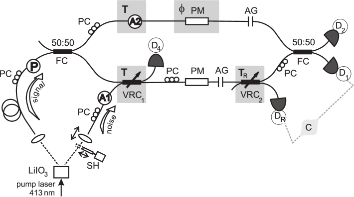
Figure 2: Experimental setup. Shutter (SH), polarization controllers (PC), polarizer (P), attenuators (A), phase modulators (PM), adjustable air-gaps (AG), fiber couplers (FC), variable-ratio couplers (VRC), detectors (D).

Signal and noise photons were created by type-I degenerate spontaneous parametric downconversion in a nonlinear crystal pumped by a continuous laser (413 nm). Photons from each pair are tightly correlated in time. They have the same polarization state and spectrum whose bandwidth is determined mainly by the coupling of photons from the nonlinear crystal into single-mode fibers.

Before the measurement the source of photon pairs was adjusted by optimizing a visibility of two-photon interference at the variable-ratio coupler VRC₁ with splitting ratio set to 50:50. The visibility of Hong-Ou-Mandel (HOM) dip [30] typically reached values about $0.98$. Then the intensities of signal and noise were balanced. It was realized by a measurement of count rates at detectors D_R and D₄ while the transmissivity of coupler VRC₂ was set to $1$. We tuned the count rates of noise at these detectors to be twice of the count rates of the signal.

Single photon visibility behind the MZ interferometer was above $0.93$.

Measurements were realized with maximally indistinguishable signal and noise photons, when HOM dip was set to its minimum. The signal to noise ratio was determined by intensity transmissivity $T$ of VRC₁. Transmissivity of the other arm of MZ interferometer was also set to the value of $T$. Coupler VRC₂ together with detector D₃, implemented the noise eater. Its transmissivity $T_{R}$ was not compensated in the other arm of interferometer.

All used detectors were Perkin-Elmer single-photon counting modules. To implement postselection measurements the signals from detectors were processed by coincidence electronics based on time-to-amplitude converters and single-channel analyzers. The coincidence window was set to 2 ns when accidental coincidence rates were negligible.

The phase of light in optical fibers is influenced by temperature changes and gradients. This undesirable phase drift was reduced by a thermal isolation of MZ interferometer and by an active stabilization of phase that was applied before each few-second measurement step.

First we measured how the visibility of interference at the outputs of MZ interferometer is damaged by the presence of noise. During this measurement no postselection was applied and so the transmissivity $T_{R}$ of VRC₂ was set to zero. It means that if the noise input is shut then the visibility at interferometer outputs maximal.

For large losses the visibility for indistinguishable and distinguishable cases degrades to the same value $V\approx T$.

The aim of this work was to increase the visibility at outputs of MZ interferometer using a coherent noise eater based on single photon subtraction. We measured coincidence rate $C_{1}$ between detectors D₁ and D_R. Intensity transmissivity of VRC₂ was adjusted to the value which maximizes the visibility of coincidence rate $C_{1}$ $T_{R}=3/4$. The visibility of $C_{1}$ was measured as a function of transmissivity $T$.

5 Experimental results

Figure 3: Dependence of visibility on transmissivity $T$. Symbols denote experimental results; circles correspond to the visibility at MZ interferometer outputs for distinguishable case and triangles for indistinguishable case, squares correspond to the visibility after recovery for indistinguishable photons. Solid lines are fits to measured data. The dashed line shows our benchmark value of visibility equal to $1/\sqrt{2}$.

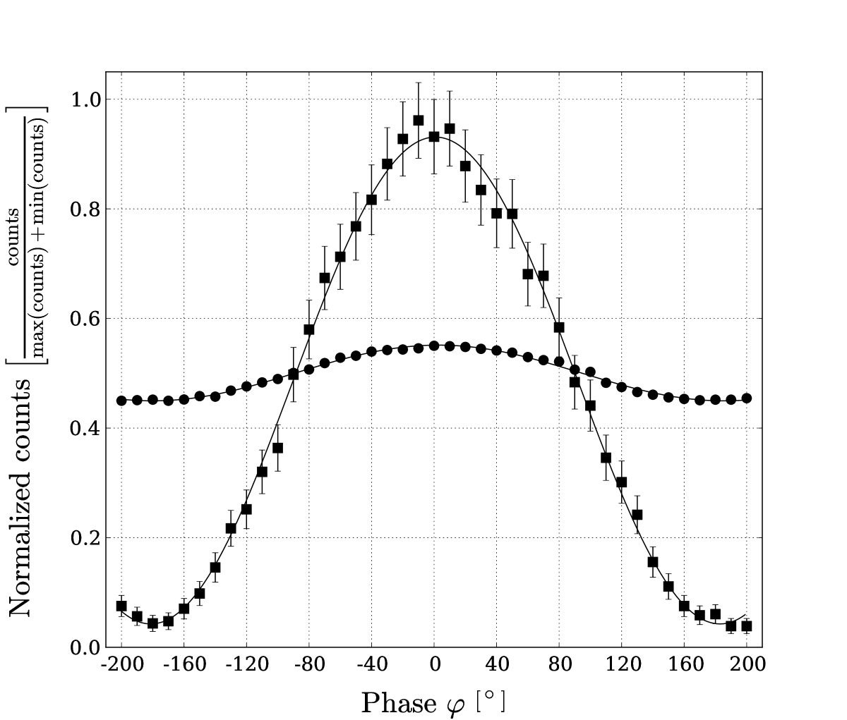
Figure 4: The interference fringes for indistinguishable photons and coupling ratio $T=0.109$. Symbols denote experimental results: circles correspond to interference fringe without correction and squares correspond to interference fringe after the recovery. Solid lines represent fits to measured data.

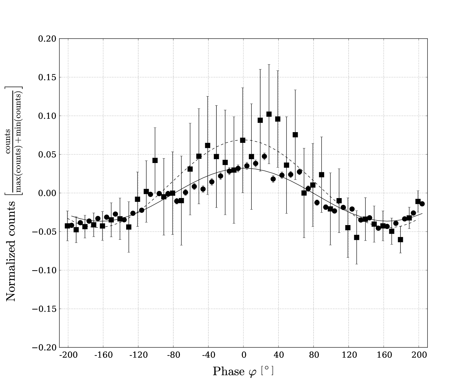
Figure 5: Circles correspond to the difference between the ideal sine interference fringe ($V=1$) and the best achieved interference fringe for $T=1$ ($V=0.936$); squares correspond to the difference between the recovered fringe for $T=0.109$ ($V=0.915$) and the ideal sine fringe ($V=1$). Solid curve corresponds to the difference between the ideal sine fringe and the fit of the best achieved interference fringe for $T=1$. Dashed curve corresponds to the difference between the ideal sine fringe and the fit of the recovered fringe for $T=0.109$.

Measured visibilities are displayed in figure 3. Interference fringes were investigated in the range of phases $[-120^{\circ},120^{\circ}]$ with a step $10^{\circ}$. Each point of interference fringe was measured 3-5 seconds, depending on a quantity of signal. Before each measurement the degree of phase drift in MZ interferometer was checked and in case of need it was minimized by a stabilization procedure. An interference fringe was measured several times. We added all these results together and then fitted data. Shown error bars are given by the Poisson distribution of photo-count statistics.

Visibility of signals at the outputs of MZ interferometer are influenced by dark counts of detectors. Hence we subtracted the minimum of corresponding dark count rates from measured count rates. Final visibilities as a functions of $T$ were fitted by the curve $a\cdot T+b$ with two parameters $a$ and $b$. Of course, parameter $a=0.936$ corresponds to the value of visibility at point $T=1$.

The other visibilities were measured in coincidence measurements and therefore no correction was needed. The visibility of coincidence rate $C_{1}$ does not depend on $T$. Obtained mean value of visibility is $0.924\pm 0.018$ (the theoretical value is 1). One can see that the fit is sometimes out of range of the error bars. It is caused by the fact that the precision of the measurement results depends on the accuracy of setting of minimum of HOM dip and on the fluctuation of this position during the measurement. The threshold value of visibility, $1/\sqrt{2}$, is plotted by a dashed line.

We have plotted an interference fringe (number of counts as a function of phase $\varphi$) for $T=0.109$ without and with recovery in the Fig. 4. To compare single photon counts and coincidence counts in one figure we have normalized them by sum of maximum counts and minimum counts measured in the range of the interference fringe. The less modulated fringe, plotted by circles, corresponds to the interference fringe measured without recovery. Visibility obtained from the fit is $0.097\pm 0.005$. If the noise eater is switched on the interference fringe becomes more modulated as is demonstrated by a curve with square symbols. The visibility increased to the value of $0.915\pm 0.017$. Shown error bars are given by Poisson distribution of photo-count statistics. The error bars significantly increase in case of a coincidence measurement. It is a consequence of the fact that the number of total counts in the coincidence detection is less then in single photon detection by two orders of magnitude in average. on average two orders less number of total counts in the coincidence detection.

In Fig. 5 we compare difference between measured and ideal interference fringes. First curve denoted by circles is a difference between an ideal sine fringe and a best achieved interference fringe for $T=1$ without the recovery ($V=0.936$). The fit to the data points is plotted by a solid line. The other curve denoted by squares corresponds to a difference between an ideal sine fringe and a best achieved fringe for $T=0.109$ with the recovery ($V=0.915$). The fit to the data points is plotted by a dashed line. The plots show that a difference between the actual fringe and the ideal sine fringe is slightly modulated. The largest differences are in maxima and minima of interference fringes. There is a greater difference between the ideal sine fringe and the fringe with the recovery than the fringe without the recovery. Also the error bars are much greater in the case of the fringe with the recovery, being again the consequence of a coincidence measurement.

6 Conclusion

We have proposed and experimentally demonstrated an elementary quantum noise eater for dual-rail qubit influenced by a randomly arriving coherent photon. The superposition of basis states carried by qubit is changed by that coherent photon and subsequently, visibility of interference of a dual-rail qubit behind the Hadamard gate is decreased. Theoretically, a perfect recovery of the superposition carried by the qubit has been predicted for the case when noise eater is applied after a coherent noise photon was randomly added. Experimentally, after the recovery we observe visibility $V=0.915$ for $T=0.109$, comparing to $V=0.097$ before the recovery, that is eight-fold increase of the visibility. The value $V=0.915$ is 12 standard deviations above the threshold, $V_{\text{th}}=1/\sqrt{2}$, for coherent noise impacts [27]. It is the first proof-of-principle test of a general quantum method of coherent noise eater for qubits which can protect qubits against coherent noise by a partial nondestructive and coherent selection of given number of photons. A weak temporal and spatial coherence of signal and noise can be enhanced by fully classical spectral filtering, as have been many times demonstrated [31, 32, 33]. It would be an interesting extension of this experiment to combine it with an induction of coherence between the qubit and noise photons. The scheme of the noise eater can also be extended to coherent noisy particle disturbing both paths of the interferometer. Required joint particle subtraction not distinguishing the paths can be implemented.

Corollary

We have also studied the action of the noise eater in a more realistic situation when noise contained more than one photon in a Fock state. We have numerically simulated behaviour of the noise eater when the signal was represented by single photon state $|1\rangle$ and to the noise port of the Mach-Zehnder interferometer was injected a state $p_{0}|0\rangle+p_{1}|1\rangle+p_{2}|2\rangle$. We have chosen the coefficients $p_{i}$ to represent the Poisson statistics in order to mimic a weak coherent state. The average number of photons in the noise mode reads $\lambda^{2}e^{-2\lambda}+(1/2)\lambda^{4}e^{-2\lambda}$, where we have used $p_{k}=\lambda^{k}e^{-\lambda}/k!$ Such a statistical model also very well corresponds to our experimental situation where we exploit the SPDC process in nonlinear crystal to create both the signal and noise states of photons. If we take into account also four-photon pairs created during the process our output state from SPDC for $\epsilon\ll 1$ reads $(1-\epsilon^{2}/2)|00\rangle+\epsilon|11\rangle+\epsilon^{2}|22\rangle$. The mean photon number generated locally in the noise mode is equal to $\epsilon^{2}+2\epsilon^{4}$. Given $\epsilon$ we can calculate the corresponding $\lambda$. We have numerically tested action of the noise eater on both states for different values of related parameters $\epsilon$ and $\lambda$. The simulation give the same results for both corresponding states. In the Fig. 6 we have plotted a result of numerical simulation for $\eta_{S}=\eta_{N}=0.001$ and $\epsilon=0.05$, which corresponds to $0.003$ average number of photons. The $T_{R}$ had to be optimized for every chosen $T$. The dashed line represents the visibility without action of the noise eater and the solid line with the action of the noise eater. Due to the presence of the two-photon events in the noise mode both curves are moved to lower values compare to single photon noise scenario studied in previous sections. But there is still a substantial improvement of the visibility after the action of the noise eater.

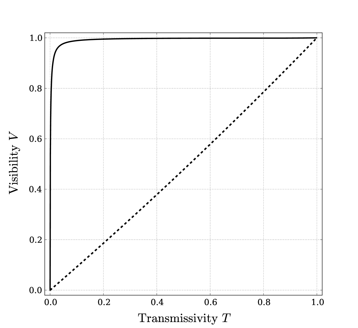
Figure 6: Numerical simulation of the noise eater when also two-photon noise contributions are present. The parameters are $\eta_{S}=\eta_{N}=0.001$, $\epsilon=0.05$ and $T_{R}$ has been optimized for every value of $T$. Dashed line represents the situation without the action of the noise eater. Solid line represents the situation with the action of the noise eater.

References

References

- [1] M. A. Nielsen, I. L. Chuang. Quantum Computation and Quantum Information, Cambridge University Press, Cambridge, 2001.
- [2] D. Bouwmeester, J.-W. Pan, K. Mattle, M. Eibl, H. Weinfurter and A. Zeilinger, Nature 390, 575-579 (1996).
- [3] I. Marcikic, H. de Riedmatten, W. Tittel, H. Zbinden and N. Gisin, Nature 421, 509-513 (2003)
- [4] E. Lombardi, F. Sciarrino, S. Popescu, and F. De Martini, Phys. Rev. Lett. 88, 070402 (2002)
- [5] J.J.L. Morton, A.M. Tyryshkin, R.M. Brown, S. Shankar, B.W. Lovett, A. Ardavan, T. Schenkel, E.E. Haller, J.W. Ager and S.A. Lyon, Nature 455, 1085-1088 (2008)
- [6] J.M. Elzerman, R. Hanson, L.H.W. Van Bereven, B. Witkamp, L.M. Vandersypen, and L.P. Kouwenhoven, Nature 430, 431 (2004).
- [7] B. Trauzettel, D.V. Bulaev, D. Loss and G. Burkard Nature Physics 3, 192 - 196 (2007)
- [8] A. Imamolu, D.D. Awschalom, G. Burkard, D.P. DiVincenzo, D. Loss, M. Sherwin, and A. Small, Phys. Rev. Lett., 83, 4204 (1999).
- [9] J. Clarke and F.K. Wilhelm, Nature 453, 1031–1042 (2008)
- [10] Y. Nakamura, Yu.A. Pashkin and J.S. Tsai, Nature 398, 786–788 (1999)
- [11] I. Chiorescu, Y. Nakamura, C.J.P.M. Harmans and J.E. Mooij, Science 299, 1869–1871 (2003)
- [12] M. Ansmann, H. Wang, R.C. Bialczak, M. Hofheinz, E. Lucero, M. Neeley, A.D. O’Connell, D. Sank, M. Weides, J. Wenner, A.N. Cleland and J.M. Martinis, Nature 461, 504–506 (2009).
- [13] K. Lemr, A. Černoch, J. Soubusta, K. Kieling, J. Eisert, and M. Dušek, Phys. Rev. Lett. 106, 013602 (2011).
- [14] M. Dall’Arno, A. Bisio, G.M. D’Ariano, M. Miková, M. Ježek, and M. Dušek, Phys. Rev. A 85, 012308 (2012).
- [15] W.H. Zurek, Rev. Mod. Phys. 75, 715–775 (2003).
- [16] A.M. Steane, Phys. Rev. Lett. 77, 793 (1996).
- [17] D. Bacon, D.A. Lidar, and K.B. Whaley, Phys. Rev. A 60, 1944 (1999)
- [18] L. Viola, S. Lloyd, and E. Knill, Phys. Rev. Lett. 83, 4888 (1999)
- [19] F. Sciarrino, E. Nagali, F. De Martini, M. Gavenda, and R. Filip, Phys. Rev. A 79, 060304 (2009).
- [20] M. Gavenda, R. Filip, E. Nagali, F. Sciarrino, and F. De Martini, Phys. Rev. A 81, 022313 (2010).
- [21] C. Weedbrook, S. Pirandola, R. Garcia-Patron, N.J. Cerf, T.C. Ralph, J.H. Shapiro, and S. Lloyd, Rev. Mod. Phys 84, 621 (2012).
- [22] B. C. Buchler, E. H. Huntington, C. C. Harb, and T. C. Ralph, Phys. Rev. A 57, 1286 (1998).
- [23] U.L. Andersen, R. Filip, J. Fiurasek, V. Josse, G. Leuchs, Phys. Rev. A 72, 060301R (2005).
- [24] M. Sabuncu, R. Filip, G. Leuchs and U.L. Andersen, Phys. Rev. A 81, 012325 (2010).
- [25] H. A. Bachor and T. C. Ralph, A Guide to Experiments in Quantum Optics, 2nd ed. Wiley-VCH, Wenheim, 2003.
- [26] C. Wittmann, D. Elser, U. L. Andersen, R. Filip, P. Marek and G. Leuchs, Phys. Rev. A 78, 032315 (2008).
- [27] M. Gavenda, L. Čelechovská, J. Soubusta, M. Dušek, and R. Filip, Phys. Rev. A 83, 042320 (2011).
- [28] D. Collins, N. Gisin, and H. de Riedmatten, J. Mod. Opt. 52, 735 (2005).
- [29] A. Martin, O. Alibart, M. P. De Micheli, D. B. Ostrowsky, and S. Tanzilli, New J. Phys. 14(2), 025002 (2012).
- [30] C.K. Hong, Z.Y. Ou, and L. Mandel, Phys. Rev. Lett. 59, 2044 (1987).
- [31] J. Soubusta, J. Peřina jr., M. Hendrych, O. Haderka, P. Trojek, and M. Dušek, Phys. Lett. A 319, 251 (2003)
- [32] M. Belllini, F. Marin, S. Viciani, A. Zavatta, and F.T. Arecchi, Phys. Rev. Lett. 90, 043602 (2003)
- [33] P. Abolghasem, M. Hendrych, X.J. Shi, J.P. Torres, and A.S. Helmy, Optics Letters 34, 2000 (2009)