Entanglement Temperature in Non-conformal Cases

Abstract

Potential reconstruction can be used to find various analytical asymptotical AdS solutions in Einstein dilation system generally. We have generated two simple solutions without physical singularity called zero temperature solutions. We also proposed a numerical way to obtain black hole solution in Einstein dilaton system with special dilaton potential. By using this method, we obtain the corresponding black hole solutions numerically and investigate the thermal stability of the black hole by comparing the free energy of thermal gas and the corresponding black hole. In two groups of non-conformal gravity solutions obtained in this paper, we find that the two thermal gas solutions are more unstable than black hole solutions respectively. Finally, we consider black hole solutions as a thermal state of zero temperature solutions to check that the first thermal dynamical law exists in entanglement system from holographic point of view.

1 Introduction

The AdS/CFT correspondence Maldacena:1997re Gubser:1998bc Witten:1998qj Aharony:1999ti is a very important and fundamental relation which connects gravitational theories and quantum field theories. As an application, in Ryu:2006bv Ryu and Takayanagi proposed a general way for calculating the entanglement entropy of boundary field theory through AdS/CFT correspondence. The main point is that the entanglement entropy in the large $N$ (and large ’t Hooft coupling) limit in field theory side can be mapped to an area of minimal surface in gravity side. Prescription on computing the holographic entanglement entropy (HEE) has been proved in Lewkowycz:2013nqa Casini:2011kv . There are so many evidences Headrick:2010zt Hartman:2013mia Faulkner:2013yia to confirm this proposal within $AdS_{3}/CFT_{2}$ correspondence. As applications of HEE, there are intensive studies Nishioka:2009un -Cai:2012es recently. More recently, in Nozaki:2013wia , a free falling particle in an AdS space was used to mimic the holographic dual of local quenches and the HEE has been computed to show the evolution of quantum entanglement. In Hartman:2013qma , an analytical framework for holographic counterpart of global quantum quenches was given. In Nozaki:2013vta , the authors studied how a small perturbation of HEE evolves dynamically through solving the Einstein equation in AdS spaces.

In vacuum state the leading divergent term of entanglement entropy(EE) is proportional to the area of the entangling surface (in many models)MBH Srednicki:1993im , which is the original motivation for relating EE with black hole entropy. The EE is also an useful quantity to describe the quantum correlations between the in and out side of a subsystem in QFT. The behavior of EE in low excited states is also important to understand the quantum entanglement nature of the system. This topic has been studied by many authors, for example FMG Masanes:2009tg . The elegant method of HEE could also be used to study the property of EE in low excited states of CFT, which may be related with the background perturbation of the bulk.

In Bhattacharya:2012mi , the authors have studied the low thermal excited state in the holographic view, and furthermore, they find an interesting relation between the variance of energy and EE of the subsystem in low thermal excited states of CFT living on the boundary, which is similar to the first law of thermodynamics, i.e., $\Delta E=T_{eff}\Delta S$, where $T_{eff}$, called entanglement temperature, is only related to the shape of the subsystem.

In effective theory of gravity, higher derivative terms will appears as corrections to Einstein-Hilbert action. The HEE formula for Lovelock gravity have been studied in deBoer:2011wk Hung:2011xb by comparing the logarithm term with the CFT prediction. Ogawa:2011fw Myers:2010xs have also studied the HEE with higher derivative gravity. In Guo:2013aca , the authors have studied the property of EE with low excitation in these cases from the the holographical point of view. Though general formula of HEE with the bulk theory containing arbitrary higher curvature terms is still an open question to be further studied, one can still hope that the results in deBoer:2011wk Hung:2011xb Chen:2013qma Bhattacharyya:2013jma Ogawa:2011fw Myers:2010xs Fursaev:2006ih Guo:2013aca will shed light on the quantum corrections to HEE. More recently, some quantum corrections have been studied in Barrella:2013wja Faulkner:2013ana .

We would like to extend these studies to non-conformal cases, especially for Einstein-dilaton system. The key point of this extension is to find vacuum state and corresponding thermal excitation state. Previously, there were various studies in Gubser-T Gursoy-T on gravity solutions in ED system. It is hard to obtain the gravity duals of these two states in these frameworks. Different from the logic of Gubser-T Gursoy-T , a bottom-up approach known as the potential reconstruction approach Farakos:2009fx Li:2011hp is indeed a much easier way to obtain gravity solutions. Using this bottom-up approach, a new Schwarzschild-AdS black hole in five-dimensions coupled to a scalar field was discussed in Farakos:2009fx , while dilatonic black hole solutions with a Gauss-Bonnet term in various dimensions were discussed in Ohta:2009pe . A new class of four dimensional gravity solutions has been found in Kolyvaris:2009pc .

We will review the potential reconstruction approach to obtain general gravity solution in 5D. In Li:2011hp , the authors have used this method to construct a semianalytical gravity solution to study some thermodynamical quantities, their results agree with the numerical results from recent studies in lattice QCD. Li:2011hp provided an excellent example of constructing a holographic model using the potential reconstruction approach. Motivated from finding the vacuum state and thermal excitation state, we would like to construct two gravity solutions or phases in the same ED system. It is valuable to study the thermal excitation properties of this system. In this paper, we will list two analytical zero temperature solutions to show the details of this approach.

In this paper, we would like try to obtain two black hole solutions which correspond to these two zero temperature solutions, respectively. To find the gravity solutions in Einstein dilation system with special dilation potential is the hard core. We here propose a systematical way to obtain the numerical gravity solutions. To give the details, we take two black hole solutions obtained in this paper as examples. Furthermore, we have studied the free energy of these solutions and find that the thermal gas solutions are thermal dynamically unstable. By following the logic line proposed by Bhattacharya:2012mi , we consider black hole solution as the thermal excitation of corresponding zero temperature solution and we would like study a novel quantity called entanglement temperature. With this entanglement temperature, there exists the first-law-like relation that are proposed in Bhattacharya:2012mi then.

The organization of the paper is as follows: in section 2, we briefly review the potential reconstruction approach to the Einstein-Maxwell-Dilaton system by generalizing the discussion in Cai:2012xh to the case with a coupling between dilaton field and Maxwell field. We also follow this approach to generate domain wall solutions. In section 3, we discuss the generic black hole solution with asymptotical AdS boundary in Einstein dilaton system, and in particular present two new analytic zero temperature solutions which will be used later. In this section, we also proposed a numerical way to obtain the black hole solutions in ED system. We list two groups of gravity solutions. In each group, the one is zero temperature solution and the other is corresponding black hole solution. In section 4, we calculate the difference of free energy of thermal gas and the corresponding black hole solutions generally. Here these thermal gas solutions are obtained from Wick rotation in time direction in zero temperature solutions. We take two groups of thermal gas and Euclidean version of black hole solutions as examples to show that the thermal gas solutions are unstable. In section 5, as an application of these solutions from AdS/CFT point of view, we study the novel quantity called entanglement temperature in these cases and we consistently check that the thermodynamical first law like exists in our cases. Section 6 is devoted to conclusions and discussions. We put some details of the computations in this paper in the Appendix A. In appendix B, we list 6 new gravity solutions generated by potential reconstruction in ED system.

2 Einstein-Maxwell-Dilaton system

In this section, we just review how to use the potential reconstruction approach Li:2011hp ; He:2010ye ; He:2011hw ; Cai:2012xh to obtain solutions to a 5D Einstein-Dilaton (ED) system and Einstein-Maxwell-Dilaton (EMD) system. In Cai:2012xh , the authors have not considered the coupling between gauge field and dilaton field in Einstein frame. Here we take the coupling into consideration to start with a more general version

$$S_{5D}=\frac{1}{16\pi G_{5}}\int d^{5}x\sqrt{-g^{S}}e^{-2\phi}\left(R^{S}+4\partial_{\mu}\phi\partial^{\mu}\phi-V_{S}(\phi)-\frac{Z(\phi)}{4g_{g}^{2}}e^{\frac{-4\phi}{3}}F_{\mu\nu}F^{\mu\nu}\right),$$ (1)

where the action (1) is written in string frame, $F_{\mu\nu}=\partial_{\mu}A_{\nu}-\partial_{\nu}A_{\mu}$ is the Maxwell field. In Einstein frame, we can write the action as He:2010ye

$$S_{5D}=\frac{1}{16\pi G_{5}}\int d^{5}x\sqrt{-g^{E}}\left(R-\frac{4}{3}\partial_{\mu}\phi\partial^{\mu}\phi-V_{E}(\phi)-\frac{Z(\phi)}{4g_{g}^{2}}F_{\mu\nu}F^{\mu\nu}\right),$$ (2)

where $V_{S}=V_{E}e^{\frac{-4\phi}{3}}.$ The metrics in both frames are connected by the scaling transformation

$$g^{S}_{\mu\nu}=e^{4\phi\over 3}g^{E}_{\mu\nu}.$$ (3)

The Einstein equations from the action (2) read

$$E_{\mu\nu}+\frac{1}{2}g^{E}_{\mu\nu}\left(\frac{4}{3}\partial_{\mu}\phi\partial^{\mu}\phi+V_{E}(\phi)\right)-\frac{4}{3}\partial_{\mu}\phi\partial_{\nu}\phi-\frac{Z(\phi)}{2g_{g}^{2}}\left(F_{\mu k}{F_{\nu}}^{k}-\frac{1}{4}g^{E}_{\mu\nu}F_{kl}F^{kl}\right)=0,$$ (4)

where $E_{\mu\nu}=R_{\mu\nu}-\frac{1}{2}Rg_{\mu\nu}$ is Einstein tensor. When we turn off the gauge field, the EDM system will be reduce to ED system given in appendix A. We here consider the ansatz $A=A_{0}(z)dt,\text{{ }}\text{{ }}\phi=\phi(z)$ for matter fields and

$$ds_{S}^{2}=\frac{{L^{2}}e^{2A_{s}}}{z^{2}}\left(-f(z)dt^{2}+\frac{dz^{2}}{f(z)}+dx^{i}dx^{i}\right),$$ (5)

for the metric in string frame, where $L$ is the radius of ${\rm AdS}_{5}$ space and $A_{s}$ is the warped factor, a function of coordinate $z$. In Einstein frame the metric reads

$$ds_{E}^{2} = \frac{{L^{2}}e^{2A_{e}}}{z^{2}}\left(-f(z)dt^{2}+\frac{dz^{2}}{f(z)}+dx^{i}dx^{i}\right),$$ (6)

$$= \frac{{L^{2}}e^{2A_{s}-\frac{4\phi}{3}}}{z^{2}}\left(-f(z)dt^{2}+\frac{dz^{2}}{f(z)}+dx^{i}dx^{i}\right),$$

with $A_{e}=A_{s}-2\phi/3$.

In the metric (6), the $(t,t),(z,z)$ and $(x_{1},x_{1})$ components of Einstein equations are respectively

$$b^{\prime\prime}(z)+\frac{b^{\prime}(z)f^{\prime}(z)}{2f(z)}-\frac{b^{\prime}(z)^{2}}{2b(z)}+\frac{4}{9}b(z)\phi^{\prime}(z)^{2}+\frac{{A_{0}}^{\prime}(z)^{2}Z(\phi)}{6g^{2}_{g}f(z)}+\frac{V_{E}(\phi)b(z)^{2}}{3f(z)}=0,$$

$$\phi^{\prime}(z)^{2}-\frac{9b^{\prime}(z)f^{\prime}(z)}{8b(z)f(z)}-\frac{9b^{\prime}(z)^{2}}{4b(z)^{2}}-\frac{3{A_{0}}^{\prime}(z)^{2}Z(\phi)}{8g^{2}_{g}b(z)f(z)}-\frac{3V_{E}(\phi)b(z)}{4f(z)}=0,$$

$$f^{\prime\prime}(z)+\frac{3b^{\prime}(z)f^{\prime}(z)}{b(z)}+\frac{4}{3}f(z)\phi^{\prime}(z)^{2}+\frac{3f(z)b^{\prime\prime}(z)}{b(z)}-\frac{3f(z)b^{\prime}(z)^{2}}{2b(z)^{2}}-\frac{{A_{0}}^{\prime}(z)^{2}Z(\phi)}{2g^{2}_{g}b(z)}+V_{E}(\phi)b(z)=0,$$

where $b(z)=\frac{L^{2}e^{2A_{e}}}{z^{2}}$, and $A_{0}(z)$ is electrical potential of Maxwell field. From those three equations one can obtain following two equations which do not contain the dilaton potential $V_{E}(\phi)$,

$$A_{s}^{\prime\prime}(z)+A_{s}^{\prime}(z)\left(\frac{4\phi^{\prime}(z)}{3}+\frac{2}{z}\right)-A_{s}^{\prime}(z)^{2}-\frac{2\phi^{\prime\prime}(z)}{3}-\frac{4\phi^{\prime}(z)}{3z}=0,$$ (8)

$$f^{\prime\prime}(z)+f^{\prime}(z)\left(3A_{s}^{\prime}(z)-2\phi^{\prime}(z)-\frac{3}{z}\right)-\frac{z^{2}Z(\phi)e^{\frac{4\phi(z)}{3}-2A_{s}(z)}A_{0}^{\prime}(z){}^{2}}{g_{g}^{2}L^{2}}=0.$$ (9)

Eq.(8) is the starting point to find exact solutions of the system. Note that Eq.(8) in the EMD system is the same as the one in the Einstein-dilaton system considered in Li:2011hp He:2011hw and the last term in Eq.(9) is an additional contribution related to electrical field. In addition, the EOM of the dilaton field is given as following

$$\frac{8}{3}\partial_{z}\left(\frac{L^{3}e^{3A_{s}(z)-2\phi}f(z)}{z^{3}}\partial_{z}\phi\right)-\frac{L^{5}e^{5A_{s}(z)-\frac{10}{3}\phi}}{z^{5}}\partial_{\phi}V_{E}(\phi)+\frac{Z^{\prime}(\phi)b(z)A_{0}^{\prime}(z)^{2}}{2g_{g}^{2}}=0.$$ (10)

The EOM of the Maxwell field is given as

$$\frac{1}{\sqrt{-g^{E}}}\partial_{\mu}\left(\sqrt{-g^{E}}Z(\phi)F^{\mu\nu}\right)=0.$$ (11)

From equations of motion, we can obtain a general solution to the system with given $A_{s}(z)$, which takes the following form

$$\phi(z) = \int_{0}^{z}\frac{e^{2A_{s}(x)}\left(\frac{3}{2}\int_{0}^{x}y^{2}e^{-2A_{s}(y)}A_{s}^{\prime}(y)^{2}\,dy+\phi_{1}\right)}{x^{2}}\,dx+\frac{3A_{s}(z)}{2}+\phi_{0},$$ (12)

$$A_{0}(z) = A_{00}+A_{01}\left(\int_{0}^{z}{ye^{\frac{2\phi(y)}{3}-A_{s}(y)}\over Z(\phi(y))}\,dy\right),$$ (13)

$$f(z) = \int_{0}^{z}x^{3}e^{2\phi(x)-3A_{s}(x)}\left(\frac{A_{01}{}^{2}\left(\int_{0}^{x}{ye^{\frac{2\phi(y)}{3}-A_{s}(y)}\over Z(\phi(y))}\,dy\right)}{g_{g}^{2}L^{2}}+f_{1}\right)dx+f_{0},$$ (14)

$$V_{E}(z) = \frac{e^{-2A_{s}(z)+\frac{4\phi(z)}{3}}z^{2}f(z)}{L^{2}}2\Big{(}-\frac{e^{-2A_{s}(z)+\frac{4\phi(z)}{3}}Z(\phi(z))z^{2}A_{0}^{\prime}(z)^{2}}{4g_{g}^{2}L^{2}f(z)}$$ (15)

$$- \frac{2\left(3+3z^{2}A_{s}^{\prime}(z)^{2}+4z\phi^{\prime}(z)+z^{2}\phi^{\prime}(z)^{2}-2zA_{s}^{\prime}(z)\left(3+2z\phi^{\prime}(z)\right)\right)}{z^{2}}$$

$$- \frac{f^{\prime}(z)\left(-3+3zA_{s}^{\prime}(z)-2z\phi^{\prime}(z)\right)}{2zf(z)}\Big{)},$$

where the $\phi_{0},A_{00},A_{01},f_{0},f_{1}$ are all integration constants and can be determined by suitable UV and IR boundary conditions. Specially for $Z(\phi)=1$, the general solution reduces to the one given in Cai:2012xh . Thus we have reviewed a generic formalism Cai:2012eh to generate exact solutions of the EMD system with a given $A_{s}(z)$.

2.1 Potential reconstruction in domain wall ansatz

By using of potential reconstruction approach, one can generate gravity solution as he/she wants. In this subsection, we do not repeat the details and just list the results.

Our starting point is the following Einstein-Maxwell-dilaton action in $d+1$ spacetime dimensions:

$$I={1\over 16\pi G_{d+1}}\int_{{\cal M}}d^{d+1}x\sqrt{-g}[R-\frac{Z(\phi)}{4}F^{2}-\frac{1}{2}(\partial\phi)^{2}+V(\phi)]+I_{GH},$$ (16)

$$I_{\text{GH}}={2\over 16\pi G_{d+1}}\int_{\partial{\cal M}}d^{d}x\sqrt{h}K.$$ (17)

This action describes the dynamics of a $U(1)$ gauge field ${\bf A}_{\mu}$ (with field strength $F=d{\bf A}$) and a real scalar field $\phi$ coupled to Einstein gravity. The boundary term $I_{\text{GH}}$ is the standard Gibbons-Hawking term needed to make the variational problem well-defined. As such this action describes the grand canonical ensemble.

Since we are interested in solutions with finite temperature and chemical potential and we set following domain wall ansatz

$$ds^{2}=e^{2A(u)}(-f(u)dt^{2}+dx^{i}dx^{i})+\frac{du^{2}}{f(u)},{\bf A}=A_{t}(u)dt,\phi=\phi(u),$$ (18)

where the AdS radius has been set to one. In this frame the second order equations of motion reduce to the following set of differential equations

$$\frac{d}{du}(e^{(d-2)A}Z\dot{A}_{t})=0,$$ (19)

$$2(d-1)\ddot{A}+\dot{\phi}^{2}=0,$$ (20)

$$\ddot{f}+d\dot{A}\dot{f}-e^{-2A}Z\dot{A}^{2}_{t}=0,$$ (21)

$$(d-1)\dot{A}\dot{f}+(d(d-1)\dot{A}^{2}-\frac{1}{2}\dot{\phi}^{2})f-V+\frac{1}{2}Ze^{-2A}\dot{A}^{2}_{t}=0.$$ (22)

Here the dot stands for derivative with respect to $u$. We can extend the logic of potential reconstruction to this general case with domain wall ansatz. The general solutions are as follows

$$A_{t}(u) = \int_{1}^{u}\frac{\rho e^{-2(A(x))}}{Z(\phi(x))}\,dx+A_{t0},$$

$$A = a_{1}u+\int_{0}^{u}\left(\int_{0}^{y}-\frac{1}{6}\phi^{\prime}(x)^{2}\,dx\right)\,dy,$$

$$f(u) = \left.\int_{0}^{u}\left(e^{-4(Ay)}\int_{0}^{y}e^{2(Ax)}\left(A_{t}(x)\right)^{2}(Z(\phi(x)))\,dx+f_{1}e^{-4(Ay)}\right)\,dy+f_{0}\right),$$

$$V(u) = (d-1)\left(A^{\prime}(u)\right)\left(f^{\prime}(u)\right)+(f(u))\left((d-1)d\left(A^{\prime}(u)\right)^{2}-\frac{1}{2}\left(\phi^{\prime}(u)\right)^{2}\right)$$ (23)

$$+ \frac{1}{2}e^{-2(A(u))}\left(A_{t}^{\prime}(u)\right)^{2}(Z(\phi(u))),$$

where $A_{t0},a_{1},f_{0},f_{1}$ are integral constants. One can use the $A(u)$ defined in (18) to generate the whole gravity solutions in terms of (2.1). As an application, we here list one explicit solution with $d=4$:

$$A(u) = u+a,$$

$$\phi(u) = b,$$

$$A_{t}(u) = -\frac{c}{2}e^{-2u},$$

$$f(u) = 1+\frac{c^{2}e^{-2a-6u}}{12}-\frac{de^{-4u}}{4}.$$

$$V(u) = 12.$$ (24)

Here $a,b,c,d$ are integral constants which can be determined by boundary conditions. One can set $a=b=c=d=0$ to reproduce the pure $AdS_{5}$ solution. This example is used to show this method is convenient to generate the gravity solution effectively.

3 General asymptotical AdS black hole solutions

In this part, we will review the general asymptotical AdS black hole solutions given in Cai:2012eh . Since we are only interested in the black hole solutions with asymptotic $AdS$ boundary, Cai:2012eh impose the boundary condition $f(0)=1$ at the AdS boundary $z=0$, and require $\phi(z),f(z),A_{0}(z)$ to be regular at black hole horizon $z_{h}$ and AdS boundary $z=0$. There is an additional condition $A_{0}(z_{h})=0$, which corresponds to the physical requirement that $A_{\mu}A^{\mu}=g^{tt}A_{0}A_{0}$ must be finite at $z=z_{h}$.

Cai:2012eh expressed the function $f(z)$ in eq.(14) as

$$f(z) = 1+\frac{A_{01}{}^{2}}{2g_{g}^{2}{L^{2}}}\frac{\int_{0}^{z}g(x)\left(\int_{0}^{z_{h}}g(r)dr\int_{r}^{x}{g(y)^{\frac{1}{3}}dy\over Z(\phi(y))}\right)dx}{\int_{0}^{z_{h}}g(x)dx}-\frac{\int_{0}^{z}g(x)dx}{\int_{0}^{z_{h}}g(x)dx},$$ (25)

where $f_{0}=1$, $f_{1}=-\frac{A_{01}{}^{2}}{4g_{g}^{2}{L^{2}}}\frac{\int_{0}^{z_{h}}g(x)\int_{0}^{x}{g(y)^{\frac{1}{3}}\over Z(\phi(y))}dy+1}{\int_{0}^{z_{h}}g(x)dx}$ and

$$g(x) = x^{3}e^{2\phi(x)-3A_{s}(x)}.$$ (26)

One can expand the gauge field near the AdS boundary to relate the two integration constants to chemical potential and charge density

$$A_{0}(z) \sim A_{00}+A_{01}{e^{\frac{2\phi(y)}{3}-A_{s}(y)}\over Z(\phi(y))}\left(1+y(\frac{2\phi^{\prime}(y)}{3}-A_{s}^{\prime}(y))\right)\Big{|}_{y=0}z^{2},$$ (27)

with

$$A_{00} = \mu,$$ (28)

$$A_{01} = \frac{\mu}{\int_{0}^{z_{h}}y{e^{\frac{2\phi}{3}-A_{s}(y)}\over Z(\phi(y))}dy}=\frac{\mu}{\int_{0}^{z_{h}}{g(y)^{\frac{1}{3}}\over Z(\phi(y))}dy}.$$ (29)

The temperature of the black hole can be determined through the function $f(z)$ in (25) as

$$T=\left|{A^{2}_{01}\over 4\pi g_{g}^{2}L^{2}}\frac{g(z_{h})\int_{0}^{z_{h}}g(r)dr\int_{r}^{z_{h}}{g^{1\over 3}(y)\over Z(\phi(y))}dy-g(z_{h})}{\int_{0}^{z_{h}}g(x)dx}\right|.$$ (30)

Following the standard Bekenstein-Hawking entropy formula, from the geometry given in eq. (6), we obtain the black hole entropy density $S$, which is obtained using the area $A_{area}$ of the horizon

$$S={\frac{A_{area}}{4G_{5}V_{3}}=\frac{L^{3}}{4G_{5}}\left(\frac{e^{A_{s}-\frac{2}{3}\phi}}{z}\right)^{3}}\Big{|}_{z_{h}},$$ (31)

where $V_{3}$ is the volume of the black hole spatial directions spanned by coordinates $x_{i}$ in (6). For this paper, we do not consider the effects of the $U(1)$ gauge field. In the remain part, we will focus on the ED system. We will propose an algorithm to obtain the black hole solution in ED system numerically. The algorithm is different from the potential construction approach shown in eq. (12)-eq. (15). Here we just review the previous results and obtain two zero temperature solutions in different ED systems. It is just technical trick to obtain zero temperature solutions. In the following subsection, we will focus on how to obtain the corresponding black hole solution numerically with respect to special zero temperature solutions in ED system.

3.1 The first analytical solution

In this subsection, we list an analytical solution of the Einstein-Maxwell-Dilaton system by using Eq.(12-15) with $Z(\phi)=1$. We impose the constrain $f(0)=1$, and require $\phi(z),f(z)$ to be regular at $z=0$, and $z_{h}$. We give the solution in Einstein frame

$$ds_{E}^{2}=\frac{{L^{2}}e^{2A_{e1}}}{z^{2}}\left(-f_{1}(z)dt^{2}+\frac{dz^{2}}{f_{1}(z)}+dx^{i}dx^{i}\right),$$ (32)

with

$$A_{e1}(z) = \log\left(\frac{z}{z_{0}\sinh(\frac{z}{z_{0}})}\right),$$

$$f_{1}(z) = 1-\frac{4V_{11}}{3}(3\sinh(\frac{z}{z_{0}})^{4}+2\sinh(\frac{z}{z_{0}})^{6})+\frac{1}{8}V_{12}^{2}\sinh\left(\frac{z}{z_{0}}\right)^{4},$$

$$\phi_{1}(z) = \frac{3z}{2z_{0}},$$

$$A_{01}(z) = \mu_{1}-\frac{2g_{g}L}{z_{0}}V_{12}\sinh\left(\frac{z}{2z_{0}}\right)^{2},$$ (33)

where $z_{0}$ is an integration constant and $V_{11},V_{12}$ are two constants from the dilaton potential

$$V_{E1}(\phi_{1}) = -\frac{12+9\sinh^{2}\left(\frac{2\phi_{1}}{3}\right)+16V_{11}\sinh^{6}\left(\frac{\phi_{1}}{3}\right)}{{L^{2}}}+\frac{V_{12}^{2}\sinh^{6}\left(\frac{2\phi_{1}}{3}\right)}{8{L^{2}}}.$$ (34)

Note that $V_{11}$ can be parameterized by black hole horizon $z_{h}$. The two integration constants $V_{11}$ and $V_{12}$ then can be expressed in terms of horizon $z_{h}$ as

$$V_{11} = \frac{3{\cosh}^{4}\left(\frac{z_{h}}{2z_{0}}\right)\left(\frac{\mu^{2}z_{0}^{2}\sinh^{4}\left(\frac{z_{h}}{z_{0}}\right){\cosh}^{4}\left(\frac{z_{h}}{2z_{0}}\right)}{4g_{g}^{2}{L^{2}}}+8\right)}{32\left(2\sinh^{2}\left(\frac{z_{h}}{2z_{0}}\right)+3\right)},$$

$$V_{12} = \frac{\mu z_{0}{\cosh}^{2}\left(\frac{z_{h}}{2z_{0}}\right)}{2g_{g}L}.$$ (35)

In this solution, we can just only consider the degenerate case with $V_{11}=0,V_{12}=0,\mu_{1}=0$. The explicit form for the degenerate case called the first zero temperature solution is

$$A_{et1}(z) = \log\left(\frac{3p_{1}z}{2\sinh(\frac{3p_{1}z}{2})}\right),$$

$$f_{t1}(z) = 1,$$

$$\phi_{t1}(z) = p_{1}z,$$

$$V_{Et1}(\phi) = -\frac{12+9\sinh^{2}\left(\frac{2\phi_{t1}}{3}\right)}{{L^{2}}}.$$ (36)

In the last step we have set $z_{0}={2\over 3}p_{1}$ which is helpful for following analysis.

3.1.1 The corresponding black hole solution

In this subsection, we would like to find the black hole solution with the same potential as the previous subsection in ED system. Firstly, the UV behavior of the black hole should be asymptotical AdS and there is a horizon in the IR region which is parameterized by $z_{h}$. We find an algorithm to find the numerical solution consistently. In order to show how the algorithm work, we list all the details in appendix. Roughly speaking, we try to expand in power series all unknown function as positive powers of $z$ and try to fix all the coefficients numerically. In the UV region, the black hole can be solved as follows from coupled equations of motion with the potential Eq. (3.1)

$$\phi_{b1}(z) = p_{1}z+p_{3}z^{3}+{((405f_{41}p_{1}+612p_{1}^{2}p_{3})z^{5})\over 3240}$$

$$+ {(8100f_{41}p1^{3}+229635f_{41}p_{3}+10944p_{1}^{4}p_{3}+133164p_{1}p_{3}^{2})z^{7}\over 612360}+O(z^{7})$$

$$f_{b1}(z) = 1-f_{41}z^{4}-{4\over 27}f_{41}p_{1}^{2}z^{6}+{-13f_{41}p_{1}^{4}\over 1215}-{f_{41}p_{1}p_{3}\over 5})z^{8}$$

$$+ {(-10935f_{41}^{2}p_{1}^{2}-328f_{41}p_{1}^{6}-37908f_{41}p_{1}^{3}p_{3}-78732f_{41}p_{3}^{2})z^{10}\over 688905}+O(z^{10})$$

$$A_{eb1}(z) = -(2/27)p_{1}^{2}z^{2}+({(4p_{1}^{4})\over 3645}-{(2p_{1}p_{3})\over 15})z^{4}$$ (37)

$$+ {(-54675f_{41}p_{1}^{2}-128p_{1}^{6}-67068p_{1}^{3}p_{3}-393660p_{3}^{2})z^{6})\over 4133430}$$

$$+ {((-50625f_{41}p_{1}^{4}+64p_{1}^{8}-3444525f_{41}p_{1}p_{3}-74952p_{1}^{5}p_{3}-2943216p_{1}^{2}p_{3}^{2})z^{8}\over 62001450}$$

$$+ O(z^{8}).$$

One can see the black hole solution in the UV region can be expressed in series of powers of $z$. In principle, one can obtain more higher powers of $z$ to get the full expression of black hole background. Unfortunately, we can not obtain complete form of the black hole solution. The main reason is that we do not find simple recurrence relation among the coefficients of each power of $z$. It is easy to see that the black hole solution with asymptotical AdS can be controlled by three integral constants $p_{1},p_{3},f_{41}$. $p_{1}$ is free parameter and $p_{3},f_{41}$ are determined by boundary condition in IR region. Here we choose parameters $p_{1},p_{3},f_{41}$ to show one black hole solution numerically. Here $p_{3},f_{41}$ are not independent and they are related to the horizon position $z_{h}$ such that $f_{b1}(z_{h})=0$. In appendix A, we will show the details how to find $z_{h}$. The numerical relation between $p_{3}(z_{h})$ and $f_{41}(z_{h})$ has been shown in Fig. 1.

Figure 1: $p_{3}\text{v.s.}f_{4}$. $p_{3}$ decreasing with $f_{41}$ monotonously. Here we have chosen the parameter $p_{1}=1.5\text{GeV}$.

For simplifying numerical analysis, we fix $p_{1}=1.5\text{GeV}$. Here we just only show the series expansion of black hole solutions and the complete solution can be obtained by the algorithm explained in appendix A. Figs. 2-4 show the configuration of black hole solution. The black hole horizon can be easily read out by $f_{b1}(z_{h})=0$. From these figures, one can continuously go back to zero temperature solution from black hole solution with decreasing value of $f_{41}$ to zero. $f_{41}$ decreases with increasing $p_{3}$ simultaneously. Where the temperature is defined by $T={{f_{b1}(z)^{\prime}\over 4\pi}|_{z=z_{h}}}$. This behavior will be helpful to understand entanglement temperature in section 5.

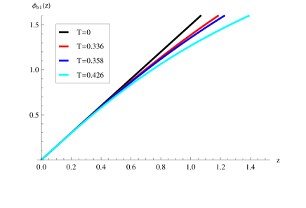
Figure 2: The configuration of $\phi_{b1}(z)$ as a function holographic coordinate $z$. Here we have fixed $p_{1}=1.5\text{GeV}$ all over the paper. The four parameters for these curves are taken values as following {${T=0,f_{41}=0,p_{3}=0}$}, {${T=0.336\text{GeV},f_{41}=0.5\text{GeV}^{4},p_{3}=-0.139...\text{GeV}^{3}}$}, {${T=0.358\text{GeV},f_{41}=0.75\text{GeV}^{4},p_{3}=-0.186...\text{GeV}^{3}}$}, {${T=0.426,f_{41}=2\text{GeV}^{4},p_{3}=-0.360...\text{GeV}^{3}}$} respectively. To get a smooth function numerically, $p_{3}$ have very high-precision and we replace the more additional number with ”…” for short.

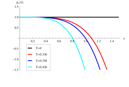
Figure 3: The configuration of $f_{b1}(z)$ as a function holographic coordinate $z$. Here we have fixed $p_{1}=1.5\text{GeV}$ all over the paper. The four parameters for these curves are taken values as following {${T=0,f_{41}=0,p_{3}=0}$}, {${T=0.336\text{GeV},f_{41}=0.5\text{GeV}^{4},p_{3}=-0.139...\text{GeV}^{3}}$}, {${T=0.358\text{GeV},f_{41}=0.75\text{GeV}^{4},p_{3}=-0.186...\text{GeV}^{3}}$}, {${T=0.426,f_{41}=2\text{GeV}^{4},p_{3}=-0.360...\text{GeV}^{3}}$} respectively. To get a smooth function numerically, $p_{3}$ have very high-precision and we replace the more additional number with ”…” for short.

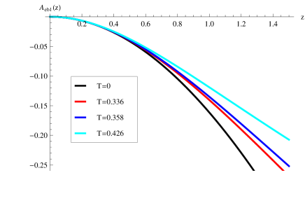
Figure 4: The configuration of $A_{eb1}(z)$ as a function holographic coordinate $z$. Here we have fixed $p_{1}=1.5\text{GeV}$ all over the paper. The four parameters for these curves are taken values as following {${T=0,f_{41}=0,p_{3}=0}$}, {${T=0.336\text{GeV},f_{41}=0.5\text{GeV}^{4},p_{3}=-0.139...\text{GeV}^{3}}$}, {${T=0.358\text{GeV},f_{41}=0.75\text{GeV}^{4},p_{3}=-0.186...\text{GeV}^{3}}$}, {${T=0.426,f_{41}=2\text{GeV}^{4},p_{3}=-0.360...\text{GeV}^{3}}$} respectively. To get a smooth function numerically, $p_{3}$ have very high-precision and we replace the more additional number with ”…” for short.

3.2 The second analytical solution

The second exact solution with ansatz

$$ds_{E}^{2}=\frac{{L^{2}}e^{2A_{e2}}}{z^{2}}\left(-f_{2}(z)dt^{2}+\frac{dz^{2}}{f_{2}(z)}+dx^{i}dx^{i}\right),$$ (38)

is

$$A_{e2}(z) = -\log\left(1+\frac{z}{z_{0}}\right),$$ (39)

$$f_{2}(z) = 1-V_{21}\left(\frac{z^{7}}{7z_{0}^{7}}+\frac{z^{6}}{2z_{0}^{6}}++\frac{3z^{5}}{5z_{0}^{5}}+\frac{z^{4}}{4z_{0}^{4}}\right)$$ (40)

$$+\frac{\rho_{2}^{2}z_{0}^{8}}{g_{g}^{2}L^{2}}\Big{(}\frac{5z^{8}}{32z_{0}^{8}}+\frac{z^{10}}{60z_{0}^{10}}+\frac{z^{9}}{12z_{0}^{9}}+\frac{11z^{7}}{84z_{0}^{7}}+\frac{z^{6}}{24z_{0}^{6}}\Big{)},$$

$$\phi_{2}(z) = 3\sqrt{2}\sinh^{-1}\left(\sqrt{\frac{z}{z_{0}}}\right),$$

$$A_{02}(z) = \mu_{2}+\rho_{2}\left(\frac{z_{0}z^{2}}{2}+\frac{z^{3}}{3}\right).$$ (41)

where $z_{0},\mu_{2},$ and $\rho_{2}$ are integration constants and $V_{21}$ is a constant from the dilaton potential and $g_{g}$ is gauge coupling. The dilaton potential is given as

$$V_{E2}(\phi_{2}) = -\frac{12}{L^{2}}-\frac{42\sinh^{4}\left(\frac{\phi_{2}}{3\sqrt{2}}\right)}{L^{2}}-\frac{42\sinh^{2}\left(\frac{\phi_{2}}{3\sqrt{2}}\right)}{L^{2}}$$ (42)

$$-\frac{3V_{21}\sinh^{14}\left(\frac{\phi_{2}}{3\sqrt{2}}\right)}{35L^{2}}-\frac{3V_{21}\sinh^{12}\left(\frac{\phi_{2}}{3\sqrt{2}}\right)}{10L^{2}}-\frac{3V_{21}\sinh^{10}\left(\frac{\phi_{2}}{3\sqrt{2}}\right)}{10L^{2}}$$

$$+\frac{\rho^{2}z_{0}^{8}}{g_{g}^{2}L^{2}}\Big{\{}\frac{\sinh^{24}\left(\frac{\phi_{2}}{3\sqrt{2}}\right)}{20L^{2}}+\frac{3\sinh^{22}\left(\frac{\phi_{2}}{3\sqrt{2}}\right)}{10L^{2}}+\frac{59\sinh^{20}\left(\frac{\phi_{2}}{3\sqrt{2}}\right)}{80L^{2}}$$

$$+\frac{15\sinh^{18}\left(\frac{\phi_{2}}{3\sqrt{2}}\right)}{16L^{2}}+\frac{5\sinh^{16}\left(\frac{\phi_{2}}{3\sqrt{2}}\right)}{8L^{2}}+\frac{5\sinh^{14}\left(\frac{\phi_{2}}{3\sqrt{2}}\right)}{28L^{2}}\Big{\}}.$$

This solution is also a generalization of the one given in Li:2011hp .

Here we turn off the $U(1)$ gauge field and the second solution can be reduced to the following

$$A_{et2}(z) = -\log\left(1+p_{1\over 2}^{2}z\right),$$ (43)

$$f_{t2}(z) = 1,$$ (44)

$$\phi_{t2}(z) = 3\sqrt{2}\sinh^{-1}\left(p_{1\over 2}\sqrt{z}\right),$$

$$V_{Et2}(\phi_{t2}) = -\frac{12}{L^{2}}-\frac{42\sinh^{4}\left(\frac{\phi_{t2}}{3\sqrt{2}}\right)}{L^{2}}-\frac{42\sinh^{2}\left(\frac{\phi_{t2}}{3\sqrt{2}}\right)}{L^{2}}.$$ (45)

Which is so called the second zero temperature solution. In the last step we have set $z_{0}={1\over\sqrt{p_{1\over 2}}}$ which is helpful for following analysis.

3.2.1 The corresponding black hole solution

In this subsection, we would like to find the black hole solution with same potential in Einstein dilation system. As before, the UV behavior of the black hole should be asymptotical AdS and there is a horizon in the IR region which is parameterized by $z_{h}$. The series expansion of solution near UV region is:

$$\phi_{b2}(z) = p_{\frac{1}{2}}\sqrt{z}-\frac{1}{108}p_{\frac{1}{2}}^{3}z^{3/2}+\frac{p_{\frac{1}{2}}^{5}z^{5/2}}{4320}+\frac{\left(653184p_{\frac{7}{2}}-5p_{\frac{1}{2}}^{7}\right)z^{7/2}}{653184}$$

$$+ \frac{z^{9/2}\left(18895680f_{42}p_{\frac{1}{2}}+515p_{\frac{1}{2}}^{9}+\frac{171}{2}\left(653184p_{\frac{7}{2}}-5p_{\frac{1}{2}}^{7}\right)p_{\frac{1}{2}}^{2}\right)}{302330880}$$

$$+ \frac{z^{11/2}\left(69284160f_{42}p_{\frac{1}{2}}^{3}+1135p_{\frac{1}{2}}^{11}+\frac{517}{2}\left(653184p_{\frac{7}{2}}-5p_{\frac{1}{2}}^{7}\right)p_{\frac{1}{2}}^{4}\right)}{13302558720}$$

$$+ O(z^{11\over 2}),$$

$$f_{b2}(z) = 1-f_{42}z^{4}-\frac{1}{15}2f_{42}p_{\frac{1}{2}}^{2}z^{5}-\frac{1}{162}f_{42}p_{\frac{1}{2}}^{4}z^{6}-\frac{f_{42}p_{\frac{1}{2}}^{6}z^{7}}{10206}$$ (46)

$$+ z^{8}\left(-\frac{f_{42}p_{\frac{1}{2}}^{8}}{1119744}-\frac{f_{42}\left(653184p_{\frac{7}{2}}-5p_{\frac{1}{2}}^{7}\right)p_{\frac{1}{2}}}{5598720}\right)$$

$$+ \frac{z^{9}\left(-35f_{42}p_{\frac{1}{2}}^{10}-7f_{42}\left(653184p_{\frac{7}{2}}-5p_{\frac{1}{2}}^{7}\right)p_{\frac{1}{2}}^{3}-839808f_{42}^{2}p_{\frac{1}{2}}^{2}\right)}{151165440}$$

$$+ O(z^{10}),$$

$$A_{eb2}(z) = -\frac{1}{18}p_{\frac{1}{2}}^{2}z+\frac{1}{648}p_{\frac{1}{2}}^{4}z^{2}-\frac{p_{\frac{1}{2}}^{6}z^{3}}{17496}+\left(\frac{p_{\frac{1}{2}}^{8}}{559872}-\frac{p_{\frac{1}{2}}\left(653184p_{\frac{7}{2}}-5p_{\frac{1}{2}}^{7}\right)}{8398080}\right)z^{4}$$ (47)

$$+ \frac{z^{5}\left(-2519424f_{42}p_{\frac{1}{2}}^{2}-109p_{\frac{1}{2}}^{10}-9\left(653184p_{\frac{7}{2}}-5p_{\frac{1}{2}}^{7}\right)p_{\frac{1}{2}}^{3}\right)}{604661760}$$

$$+ \frac{z^{6}\left(-37791360f_{42}p_{\frac{1}{2}}^{4}+325p_{\frac{1}{2}}^{12}-159\left(653184p_{\frac{7}{2}}-5p_{\frac{1}{2}}^{7}\right)p_{\frac{1}{2}}^{5}\right)}{228562145280}$$

$$+ O(z^{6}).$$

One can see the black hole solution in the UV region can be expressed in series of powers of $z$. In principle, one can obtain more higher powers of $z$ to produce the full expression of black hole background. Unfortunately, we can not obtain complete form of the black hole solution. The main reason is still that we also do not find recurrence relation among the coefficients of each power of $z$. It is easy to see that the black hole solution with asymptotical AdS can be controlled by three integral constants $p_{1\over 2},p_{7\over 2},f_{42}$. $p_{1\over 2}$ is free and $p_{1\over 2},p_{7\over 2},f_{42}$ are determined by boundary condition in IR region. In this case, $p_{7\over 2},f_{42}$ are not independent and they are determined by the black hole horizon $z_{h}$. The numerical relation between $p_{7\over 2}$ and $f_{42}$ has been shown in Fig. 5.

Figure 5: $p_{7\over 2}\text{v.s.}f_{42}$. $p_{7\over 2}$ decreasing with $f_{42}$ monotonously. Here we have chosen the parameter $p_{1\over 2}=1\text{GeV}$.

For simplifying, we choose groups of $p_{1\over 2}=1\text{GeV}^{1\over 2}$ in this paper. Here we fix parameters $p_{7\over 2},f_{42}$ to show black hole solutions numerically in Fig. 6-8. Finally, one can obtain the zero temperature solution with setting $p_{1\over 2}=1\text{GeV}^{1\over 2},p_{7\over 2}=0,f_{42}=0$. Tuning on $p_{7\over 2},f_{42}$ correspond to thermal excitation of zero temperature solution and one also have seen this phenomenon in the first group of solution. In the next section, we will calculate the difference of free energy between the Euclidean black hole and thermal gas obtained by Euclidean zero temperature solution to prove thermal gas is more unstable than black hole. In this case, turning on small value of $f_{42}$ correspond the thermal excitation from zero temperature solution. Simultaneously, $f_{42}$ increases from zero to small positive value corresponds that decreasing $p_{7\over 2}$ from zero to small negative number. That is to say the black hole solution can be degenerated to zero temperature solution continuously with setting $f_{42}=0,p_{7\over 2}=0$.Where the temperature is defined by $T={{f_{b2}(z)^{\prime}\over 4\pi}|_{z=z_{h}}}$. Similar consequence applies for the first group of solutions.

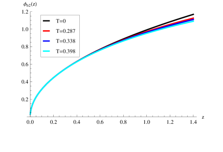
Figure 6: The configuration of $\phi_{b2}(z)$ as a function holographic coordinate $z$. Here we have fixed $p_{1\over 2}=1\text{GeV}^{1\over 2}$ all over the paper, and the four curves’ parameters is as following {${T=0,f_{42}=0,p_{7\over 2}=0}$}, {${T=0.287\text{GeV},f_{42}=0.5\text{GeV}^{4},p_{7\over 2}=-0.040...\text{GeV}^{7\over 2}}$}, {${T=0.338\text{GeV},f_{42}=1.0\text{GeV}^{4},p_{7\over 2}=-0.070...\text{GeV}^{7\over 2}}$}, {${T=0.398\text{GeV},f_{42}=2.0\text{GeV}^{4},p_{7\over 2}=-0.121...\text{GeV}^{7\over 2}}$}. To get a smooth function numerically, $p_{7\over 2}$ have very high-precision and we replace the more additional number with ”…” for short.

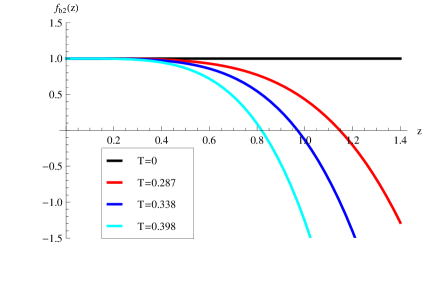
Figure 7: The configuration of $f_{b2}(z)$ as a function holographic coordinate $z$. Here we have fixed $p_{1\over 2}=1\text{GeV}^{1\over 2}$ all over the paper, and the four curves’ parameters is as following {${T=0,f_{42}=0,p_{7\over 2}=0}$}, {${T=0.287\text{GeV},f_{42}=0.5\text{GeV}^{4},p_{7\over 2}=-0.040...\text{GeV}^{7\over 2}}$}, {${T=0.338\text{GeV},f_{42}=1.0\text{GeV}^{4},p_{7\over 2}=-0.070...\text{GeV}^{7\over 2}}$}, {${T=0.398\text{GeV},f_{42}=2.0\text{GeV}^{4},p_{7\over 2}=-0.121...\text{GeV}^{7\over 2}}$}. To get a smooth function numerically, $p_{7\over 2}$ have very high-precision and we replace the more additional number with ”…” for short.

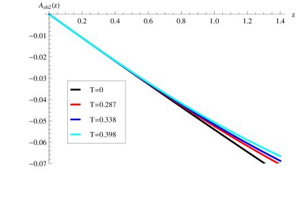
Figure 8: The configuration of $A_{eb2}(z)$ as a function holographic coordinate $z$. Here we have fixed $p_{1\over 2}=1\text{GeV}^{1\over 2}$ all over the paper, and the four curves’ parameters is as following {${T=0,f_{42}=0,p_{7\over 2}=0}$}, {${T=0.287\text{GeV},f_{42}=0.5\text{GeV}^{4},p_{7\over 2}=-0.040...\text{GeV}^{7\over 2}}$}, {${T=0.338\text{GeV},f_{42}=1.0\text{GeV}^{4},p_{7\over 2}=-0.070...\text{GeV}^{7\over 2}}$}, {${T=0.398\text{GeV},f_{42}=2.0\text{GeV}^{4},p_{7\over 2}=-0.121...\text{GeV}^{7\over 2}}$}. To get a smooth function numerically, $p_{7\over 2}$ have very high-precision and we replace the more additional number with ”…” for short.

4 Energy momentum tensor and free energy

In this section, we would like to study the stability of thermal gas solutions and Euclidean black hole solutions by comparing the free energy. Here we should stress that thermal gas solution is obtained by Euclidean version of zero temperature solution as mentioned previously Gursoy:2008za . To obtain reasonable energy momentum tensor on the boundary, one should introduce the suitable counter terms. For later use, we just focus on these two groups of thermal gas solutions and black hole solutions. One will see these two groups of solutions capture different characters of UV behaviors. These characters will lead to different behaviors of entanglement temperature which will be studied in the next section.

4.1 Energy momentum tensor

In this subsection, we would like to introduce the counter terms to cancel the divergent of the action and make the energy momentum tensor of dual field theory well defined. In our cases, one can find that we have to introduce $\phi^{2},\phi^{4},\phi^{6}$ terms to cancel the divergences. For $\phi^{2}$ term, it is introduced as standard AdS/CFT dictionary to make the energy momentum tensor of dual field theory be well defined. These additional terms related to $\phi^{4},\phi^{6}$ will be helpful to give to well defined boundary energy momentum tensor for the second black hole solution. The total action now becomes

$$I_{\text{ren}} = S_{\text{5D}}+S_{\text{GH}}+S_{\text{count}}$$

$$= \frac{1}{16\pi G_{5}}\int_{M}d^{5}x\sqrt{-g^{E}}\left(R-\frac{4}{3}\partial_{\mu}\phi\partial^{\mu}\phi-V_{E}(\phi)-\frac{Z(\phi)}{4g_{g}^{2}}F_{\mu\nu}F^{\mu\nu}\right)$$

$$- \frac{1}{16\pi G_{5}}\int_{\partial M}d^{4}x\sqrt{-\gamma}\Big{[}2K-{6\over L}+{8\lambda_{2}\phi^{2}\over 3L}+{64\lambda_{4}\phi^{4}\over 9L^{2}}+{512\lambda_{6}\phi^{6}\over 81L^{3}}\Big{]},$$

with $\lambda_{2},\lambda_{4},\lambda_{6}$ are coefficients of count terms $\phi^{2},\phi^{4},\phi^{6}$ introduced here. These coefficients can be fixed by canceling the divergences of boundary momentum tensor. Here $K_{ij}$ and $K$ are respectively the extrinsic curvature and its trace of the boundary $\partial M$, $\gamma_{ij}$ is the induced metric on the boundary $\partial M$. These quantities are defined as follows

$$\gamma_{\mu\nu} = g_{\mu\nu}+n_{\mu}n_{\nu},$$ (49)

$$K_{\mu\nu} = h^{\lambda}_{\nu}D_{\lambda}n_{\mu},$$ (50)

$$\gamma = \det(\gamma_{\mu\nu}),$$ (51)

$$K = g^{\mu\nu}K_{\mu\nu},$$ (52)

where $\gamma_{\mu\nu}$ denotes the induced metric, $n_{\mu}$ stands for the normal direction to the boundary surface $\partial M$ as well as $D_{\lambda}$ stands for covariant derivative.

In the asymptotical AdS space, the boundary surface locates at $z=0$ surface, and usually one has to regularized it to a finite $z=\epsilon$ surface. So we have the normalized normal vector $n_{\mu}=\frac{\delta^{\mu}_{z}}{\sqrt{g_{zz}}}$.

The first term of the last line in (4.1) is Gibbons-Hawking term $S_{\text{GH}}$ and the remain terms are related to counter terms $S_{\text{count}}$ related to cosmological constant and dilaton field.

To regulate the theory, we restrict to the region $z\geq\epsilon$ and the surface term is evaluated at $z=\epsilon$. The induced metric is $\gamma_{ij}=\frac{\tilde{L}^{2}}{\epsilon^{2}}g_{ij}(x,\epsilon)$, where the leading term of expansion of $g_{ij}(x,\epsilon)$ with respect to $\epsilon$ is the flat metric $g_{(0)}^{ij}$. Then the one point function of stress-energy tensor of the dual CFT is given by KS SKS

$$T_{ij}=\frac{2}{\sqrt{-\det g_{(0)}}}\frac{\delta I_{ren}}{\delta g_{(0)}^{ij}}=\lim_{\epsilon\to 0}\Big{(}\frac{{L}^{2}}{\epsilon^{2}}\frac{2}{\sqrt{-\gamma}}\frac{\delta I_{ren}}{\delta\gamma^{ij}}\Big{)}.$$ (53)

The finite part of boundary energy-stress tensor is from the $O(\epsilon^{2})$ of the Brown-York tensor $T^{BY}_{ij}$ on the boundary $z=\epsilon$, with

$$T^{BY}_{ij}=-\frac{1}{16\pi G_{5}}\Big{[}(K_{ij}-(K+{d-2\over L}+{\lambda_{2}\over L}\phi(\epsilon)^{2}+{\lambda_{4}\over L^{2}}\phi(\epsilon)^{4}+{\lambda_{6}\over L^{3}}\phi(\epsilon)^{6})\gamma_{ij})\Big{]},$$ (54)

In the first black solution, the coefficients of count terms can be following

$$\lambda_{2} = {1\over 4},$$

$$\lambda_{4} = 0,$$

$$\lambda_{6} = 0.$$ (55)

Directly evaluate (54) using (53), we get

$$T_{tt}={L^{3}\over 16\pi G_{5}}{}({3\over 2}f_{41}-p_{1}({2p_{1}^{3}\over 81}+{2\over 3}p_{3})).$$ (56)

One can see we can only introduce the $\phi^{2}$ term to cancel the action to make the boundary energy momentum tensor be well defined. These higher powers of $\phi$, such as $\phi^{4},\phi^{6}$ terms, are not necessary to be included.

The $tt$ component of energy tensor on the UV boundary of the second black hole solution

$$T_{tt}={L^{3}\over 16\pi G_{5}}\left(\frac{3f_{42}}{2}-\frac{p_{{1\over 2}}^{8}}{5511240}-\frac{p_{{1\over 2}}p_{{7\over 2}}}{2}\right).$$ (57)

To obtain the well defined boundary energy momentum tensor, it is necessary to introduce $\phi^{2},\phi^{4},\phi^{6}$ terms. The coefficients of these terms can be determined by canceling the divergences of boundary energy momentum tensor. In this case, one should introduce the additional term $\phi^{4},\phi^{6}$ terms to obtain the finite boundary momentum tensor. This aspect is different from the previous case. Here we list the coefficients of related counter terms

$$\lambda_{2} = {1\over 8},$$

$$\lambda_{4} = {L\over 1152},$$

$$\lambda_{6} = {L^{2}\over 414720}.$$ (58)

In terms of the results, one can introduce more powers of $\phi$ terms as a strategy to cancel the divergences of boundary energy momentum tensor for more general Einstein dilaton system. Here we just only take two groups of solutions as examples to show how to obtain the finite energy momentum tensor on the boundary.

4.2 The difference of free energy

In this subsection, we would like to study the difference of free energy between thermal gas and Euclidean black hole. In terms of total Euclidean action given in (4.1), we can obtain on-shell action for black hole as following

$$S_{\text{5D-BH}} = 2\int d^{3}x\int^{\beta}_{0}d\tau\int^{z_{h}}_{0}dz\partial_{z}(b_{eb}^{2}b_{eb}^{{}^{\prime}}f_{b})=2V_{3}\beta(b_{eb}^{2}b_{eb}^{{}^{\prime}}f)|_{\epsilon}^{z_{h}}$$

$$S_{\text{GH-BH}} = V_{3}\beta\Big{(}b_{eb}^{3}(\epsilon)f^{\prime}_{b}(\epsilon)+8b_{eb}^{2}(\epsilon)b^{\prime}_{eb}(\epsilon)f_{b}(\epsilon)\Big{)}$$ (59)

with $b_{eb}(z)={e^{A_{eb}(z)}\over z}={e^{A_{sb}(z)-{2\over 3}\phi_{b}(z)}\over z}$, the period of Euclidean time ${\beta}={1\over T}$ and volume of space ${V_{3}}$. Here $S_{\text{BHcount}}$ is given by (4.1) with insertion of thermal gas solution and $\epsilon$ is the regularized point. Here we also used eqs.(A.81) and (A.100) to obtain (4.2). Due to that $\phi_{b}$ satisfies the asymptotical AdS boundary condition, $S_{\text{BHcount}}=0$. Hence it is not necessary to consider the contribution from $S_{\text{BHcount}}$.

Figure 9: The difference of free energy of black hole and thermal gas in the first group solution. Here we choose the parameter $p_{1}=1.5\text{GeV}$.

Figure 10: The difference of free energy of black hole and thermal gas in the second group. Here we choose the parameter $p_{1\over 2}=1\text{GeV}^{1\over 2}$.

In term of (4.2), one replace $A_{eb},f_{b}$ with $A_{et},f_{t}$ to calculate the free energy of thermal gas which is only dependent on UV behavior of conformal factor $b_{et}(z)$ in the following way

$$S_{\text{TG}}^{\text{reg}} = S_{\text{5D-TG}}+S_{\text{GH}}+S_{\text{TGcount}},$$ (60)

$$= \frac{1}{16\pi G_{5}}\lim_{\tilde{\epsilon}\mapsto 0}\tilde{\beta}(\tilde{\epsilon})\tilde{V}_{3}(\tilde{\epsilon})\Big{(}6b_{et}^{2}(\tilde{\epsilon})b_{et}^{\prime}(\tilde{\epsilon})\Big{)}+S_{\text{TGcount}},$$

with $b_{et}={e^{A_{et}}\over z}$, the period of Euclidean time $\tilde{\beta}={1\over T}$ and volume of space $\tilde{V_{3}}$. Where $S_{\text{TGcount}}$ is given by (4.1) with insertion of thermal gas solution. We have checked that for thermal gas solution, the integral of the Einstein-Hilbert action extends on the region $(0,z_{IR})$, where $z_{IR}$ is the IR cutoff and the IR contribution vanishes whenever $6b_{et}^{2}(z_{IR})b_{et}^{\prime}(z_{IR})\rightarrow 0$ as $z\rightarrow z_{IR}$. For these two thermal gas solutions, the IR contribution vanishes as $z\rightarrow z_{IR}$. Due to the fact that $\phi_{t}$ satisfy with the asymptotical AdS boundary condition, $S_{\text{TGcount}}=0$. Here it is not necessary to consider the contribution from $S_{\text{TGcount}}$.

In order to compare the free energy between black hole and thermal gas, we should match the following conditionsGursoy:2008za

$$b_{et}(\tilde{\epsilon})\tilde{\beta}(\tilde{\epsilon})=b_{eb}(\epsilon)\beta(\epsilon)\sqrt{g(\epsilon)},\text{ }\text{ }\text{ }\text{ }{b}_{et}(\tilde{\epsilon})^{3}\tilde{V}_{3}(\tilde{\epsilon})=b_{eb}(\epsilon)^{3}V_{3}(\epsilon).$$ (61)

Here $\epsilon,\tilde{\epsilon}$ are different UV cutoff in black hole and thermal gas solution respectively. One should match $\phi_{th}(\tilde{\epsilon})=\phi_{b}(\epsilon)$ to obtain the relationship between $\epsilon$ and $\tilde{\epsilon}$. In terms of the relationship, one can obtain the difference of on shell action between thermal gas and black hole

$$S_{\text{BH-TG}} = -\frac{\beta V_{3}}{16\pi G_{5}}\Big{(}\lim_{\epsilon\mapsto 0}\Big{(}b_{eb}^{3}(\epsilon)f^{\prime}_{b}(\epsilon)+6b_{eb}^{2}(\epsilon)b^{\prime}_{eb}(\epsilon)f_{b}(\epsilon)\Big{)}+S_{\text{BHcount}}\Big{)}$$ (62)

$$+\Big{(}{b_{eb}^{4}(\epsilon)\sqrt{f_{b}(\epsilon)}\over b_{et}^{4}(\tilde{\epsilon})}6b_{et}^{2}(\tilde{\epsilon})b_{et}^{\prime}(\tilde{\epsilon})+S_{\text{TGcount}}\Big{)}.$$

One can see the formula (62) is consistent with on shell action Cai:2012xh in EDM system with $U(1)$ gauge field turned off. The difference of free energy $\beta\Delta F=S_{\text{BH-TG}}$ between thermal gas and black hole are always negative as shown in Fig. 9 and 10 which correspond to the first and second group of solutions respectively. Here the $\Delta F$ denotes the difference of free energies between them. In Fig. 9 and 10, we just set parameters to show the difference of free energy between black hole and thermal gas. As we can see in Fig. 9 and 10, the black hole solutions will go back to thermal gas solution when the temperature decreases to zero. In the whole region $T\geq 0$, black holes solutions are favored in these two groups of solutions. Here one should note that these thermal gas solutions are obtained by compactifying the time direction into a circle without considering back reaction of equation of state of thermal gas. Therefore, black hole phases is more stable than thermal gas phases in these two groups of gravity solutions as shown in Fig. 9 and 10 in this level. We also wound like to mention that in Fig. 9 and 10, $\Delta F$ is always negative although its absolute value is very small when $T$ is not large enough.

5 Entanglement temperature

As applications of these solutions from AdS/CFT point of view, we consider the novel quantity called entanglement temperature in non-conformal cases Klebanov:2007ws Ryu:2006ef Narayan:2013qga for our solutions. It is highly nontrivial to consider the dynamical entanglement temperature. Now we have generated two zero temperature solutions and the corresponding black hole solutions. Previous studies in above sections have shown that the black hole solutions can go back to zero temperature solutions. In this sense, that is to say black hole solutions are thermal states of zero temperature solutions in our cases. It is necessary to check whether there exists the first law of thermodynamics for EE in this system.

5.1 Variation of entanglement entropy in strip case

In this subsection, we consider the subsystem with a stripe profile which is defined by $-\frac{L_{s}}{2}<x_{1}\equiv x<\frac{L_{s}}{2}$ and $-\frac{R_{0}}{2}<x_{2},x_{3}<\frac{R_{0}}{2}$ where $R_{0}$, as a cutoff, is the lengthes of $x_{2},x_{3}$ direction. Then the induced metric $h_{\mu\nu}$ of the bulk surface after perturbation (or thermal excitation) in the Einstein frame is

$${L^{2}e^{2A_{e}(z)}\over z^{2}}\Big{(}{1\over f(z)}+x^{\prime}(z)^{2}\Big{)}dz^{2}+\Big{(}{L^{2}e^{2A_{e}(z)}\over z^{2}}\Big{)}dx_{1}^{2}+\Big{(}{L^{2}e^{2A_{e}(z)}\over z^{2}}\Big{)}dx_{2}^{2},$$

where $x$ is a function of $z$, $x=x(z)$ and the prime stands for the derivative with respect to $z$ in this subsection. We get the following volume of the submanifold which can thought as an action

$$S={L^{3}R_{0}^{2}\over 16\pi G_{5}}\int dz{1\over z^{3}}\sqrt{{e^{6A_{e}(z)}(1+f(z)x^{\prime}(z)^{2})\over f(z)}}.$$ (64)

By minimizing the functional (64) to obtain the classical configuration, we get the following equation of motion

$$x^{\prime\prime}(z) + \frac{f(z)x^{\prime}(z)^{3}\left(3zA_{e}^{\prime}(z)-3\right)}{z}$$ (65)

$$+ \frac{x^{\prime}(z)\left(2f(z)\left(3zA_{e}^{\prime}(z)-3\right)+zf^{\prime}(z)\right)}{2zf(z)}=0.$$

The solution is

$$L_{s}(z_{0}) = 2\int_{0}^{z_{0}}{z^{3}\over\sqrt{(e^{6A_{e}(z)-6A_{e}(z_{0})}z_{0}^{6}-z^{6})f(z)}}dz$$ (66)

$$= 2z_{0}\int_{0}^{1}{t^{3}\over\sqrt{(e^{6A_{e}(z_{0}t)-6A_{e}(z_{0})}-t^{6})f(z_{0}t)}}dt,$$

where $z_{0}$ is the maximal value of $z$ on the surface in the bulk, which is also called the turning point. Here the turning point is defined by $x^{\prime}|_{z=z_{0}}=\infty$ and the boundary conditions give $x|_{z=0}=\pm L_{s}/2$. We only care about the case that the size $L_{s}$ of subsystem satisfies $L_{s}\ll R_{0}$ which means $z_{0}\ll R_{0}$. We have checked that $L_{s}(z_{0})$ is monotonic function of $z_{0}$ numerically. And one can show that $z_{0}\ll R_{0}$ is equivalent to $L_{s}\ll R_{0}$.

Under this approximation, eq. (66) can be expressed by following simple form.

$$L_{s}(z_{0})=\frac{2\sqrt{\pi}\Gamma\left(\frac{2}{3}\right)z_{0}}{\sqrt{f_{\text{b,th}}(0)}\Gamma\left(\frac{1}{6}\right)}+O(z_{0}),$$ (67)

where $f(z)=f_{\text{b,th}}$ correspond to configuration of black hole and zero temperature solution respectively. We have expanded the integrand in (66) in power series of $z_{0}$ and performed the integration to obtain the $L_{s}(z_{0})$ in case of $z_{0}\ll R_{0}$.

The entanglement entropy in zero temperature solution is

$$S_{th} = \frac{L^{3}R_{0}^{2}}{8\pi G_{5}}\int_{0}^{z_{0}}{dz\over z^{3}}\sqrt{\frac{z_{0}^{6}e^{12A_{et}(z)}}{f_{th}(z)\left(z_{0}^{6}e^{6f_{t}(z)}-z^{6}e^{6A_{et}(z_{0})}\right)}}$$ (68)

$$= \frac{L^{3}R_{0}^{2}}{8\pi G_{5}z_{0}^{2}}\int_{0}^{1}{dt\over t^{3}}\sqrt{\frac{z_{0}^{6}e^{12A_{et}(z_{0}t)}}{f_{t}(z_{0}t)\left(z_{0}^{6}e^{6f_{t}(z_{0}t)}-(z_{0}t)^{6}e^{6A_{et}(z_{0})}\right)}}$$

The entanglement entropy $S_{b}$ in black hole can be obtained by replace $A_{eth},\phi_{th},f_{th}$ with $A_{eb},\phi_{b},f_{b}$. Here $S_{th},S_{b}$ have not been regularized. If one is only interested in the variation of entanglement entropy, one can find that the two integrands in $S_{th},S_{b}$ have the same behavior near $z\sim 0$.

Now we introduce the counter terms for $S_{th}$ to resolve the divergent of integrand at $t=0$,

$$S_{\text{thEEcout}} = \frac{L^{3}R_{0}^{2}}{8\pi G_{5}}\int_{0}^{1}dt\Big{(}\frac{e^{3A_{et}(0)}}{\sqrt{f_{t}(0)}t^{3}z_{0}^{2}}+\frac{e^{3A_{et}(0)}\left(6f_{t}(0)A_{et}^{\prime}(0)-f_{t}^{\prime}(0)\right)}{2f_{t}(0)^{3/2}t^{2}z_{0}}$$ (69)

$$+ \frac{e^{3A_{et}(0)}\left(-12f_{t}(0)f_{t}^{\prime}(0)A_{et}^{\prime}(0)+36f_{t}(0)^{2}A_{et}^{\prime}(0){}^{2}\right)}{8f_{t}(0)^{5/2}t}$$

$$+ \frac{e^{3A_{et}(0)}\left(12f_{t}(0)^{2}A_{et}^{\prime\prime}(0)-2f_{t}(0)f_{t}^{\prime\prime}(0)+3f_{t}^{\prime}(0)^{2}\right)}{8f_{t}(0)^{5/2}t}\Big{)}$$

$$+ \Big{(}-\frac{e^{3A_{et}(0)}\left(6f_{t}(0)z_{0}A_{et}^{\prime}(0)-z_{0}f_{t}^{\prime}(0)+f_{t}(0)\right)}{2f_{t}(0)^{3/2}z_{0}^{2}}\Big{)}$$

Where the final term comes from compensation to deal with divergent. Combining (68) and (69) will lead to $S^{reg}_{th}=S_{th}-S_{\text{thEEcout}}$ with putting the geometrical functions $A_{et}=A_{etn},f_{t}=f_{tn},\phi_{t}=\phi_{tn}$ with $n=1,2$. In term of (68) and (69), one just only replace $A_{et},f_{t}$ with $A_{eb},f_{b}$ to obtain $S^{reg}_{b}$. Finally, the variation of entanglement entropy

$$\Delta S=S^{reg}_{b}-S^{reg}_{th}.$$ (70)

In the following part, we consider the black hole as low thermal excitation of zero temperature solution and calculate the difference of entanglement entropy between them approximately.

5.2 Entanglement temperature in strip case

Bhattacharya:2012mi has proposed a universal relation between the variance of the energy and the entanglement entropy for a small subsystem on the boundary theory. The universal relation induce a novel concept called entanglement temperature. The $t-t$ component of the energy-stress tensor KS SKS corresponds to the energy density (56) and (57) in first and second black hole solution respectively.

For the finite stripe, the variance of entanglement entropy (70) in the subsystem of the first group of gravity solutions is

$$\Delta S_{fst} = {(0.350546f_{41}-0.409903p_{1}p_{3})L^{3}R_{0}^{2}\over 8\pi G_{5}}z_{0}$$ (71)

$$= {(0.350546f_{41}-0.409903p_{1}p_{3})L^{3}R_{0}^{2}\over 8\pi G_{5}}{L_{s}^{{2}}\Gamma({1\over 6})^{{2}}\over\pi^{{2}}\Gamma({2\over 3})^{{2}}}.$$

Where $p_{t1}=p_{b1}=p_{1},f_{t41}=0,p_{3}=0$ and $f_{b41}=f_{41},p_{b3}=p_{3}$ . On the other hand, the increased amount of energy in the subsystem with strip configuration is given by

$$\Delta E = \int dx^{3}\left(T_{tt}^{b1}-T_{tt}^{t1}\right),$$ (72)

$$= {L^{3}R_{0}^{2}L_{s}\over 8\pi G_{5}}{}({3\over 2}f_{41}-{2\over 3}p_{1}p_{3}).$$

Where $T_{tt}^{b1}$ and $T_{tt}^{t1}$ stand for the $tt$ component of boundary energy momentum tensor in black hole and zero temperature in first group solutions respectively. For the exact formula about $T_{tt}$, we refer to eq. (56). For $p_{1}=0$, the first zero temperature solution and the first black hole solution will go back to the case Bhattacharya:2012mi and the variation of entanglement entropy and boundary energy momentum tensor also reproduce boundary momentum tensor given in Bhattacharya:2012mi .

The entanglement temperature in the first black hole is

$$\frac{1}{T_{ent}} = {\Delta S_{fst}\over\Delta E_{fst}}$$ (73)

$$= {(0.350546f_{41}-0.409903p_{1}p_{3})\over({3\over 2}f_{41}-{2\over 3}p_{1}p_{3})}{L_{s}\Gamma({1\over 6})^{{2}}\over\pi^{{2}}\Gamma({2\over 3})^{{2}}}.$$

One can find that the ${T_{ent}}\sim[E]$ through dimensional analysis with $[f_{41}]=[E^{4}],[p_{1}]=[E^{1}],[p_{3}]=[E^{3}],[L_{s}]=[E^{-1}]$. Here $R_{0}$ is considered as the character length of the subsystem on the boundary. In terms of the dimensional analysis, one can see the coefficient highly depends on the geometry and shape of strip. In the first group of solutions, we fix the $p_{1}=1.5GeV$ for convenience to study the entanglement temperature without loss of generality. From our numerical study, $f_{41},p_{3}$ are not independent and they are fixed by horizon condition $f(z_{h})=0$. In this sense, $f_{41},p_{3}$ are functions of the position of black hole horizon $z_{h}$ or black hole temperature. In our cases, we just only turn on small $f_{41}$ or $p_{3}$ to control the temperature shown in Fig. 11. The temperature $T={{f_{b1}(z)^{\prime}\over 4\pi}|_{z=z_{h}}}$ increases with $f_{41}$ and $p_{3}$ decreases simultaneously in the first black hole solution. The temperature goes from zero to small positive value which corresponds to that $f_{41}$ increases from zero to small positive value. At the same time, the behavior of $p_{3}$ decreases from zero to negative value monotonically. In terms of (73), both of the nominator and denominator in (73) are all positive and the entanglement temperature are positive which is consistent with thermodynamical first law like proposed by Bhattacharya:2012mi .

Figure 11: T v.s. $f_{41}$ in the first solution when $p_{1}=1.5\text{GeV}$.

For the finite stripe, the variance of entanglement entropy (70) in the subsystem of the second background is

$$\Delta S_{snd} = {(0.350546f_{42}-0.23911p_{{7\over 2}}p_{1\over 2})L^{3}R_{0}^{2}\over 8\pi G_{5}}z_{0}^{{3\over 2}}$$ (74)

$$= {(0.350546f_{42}-0.23911p_{{7\over 2}}p_{1\over 2})L^{3}R_{0}^{2}\over 8\pi G_{5}}{L_{s}^{{2}}\Gamma({1\over 6})^{{2}}\over\pi^{{2}}\Gamma({2\over 3})^{{2}}}.$$

Where $p_{t2}=p_{b21}=p_{2},f_{t42}=0,p_{7t\over 2}=0$ and $f_{b42}=f_{42},p_{7b\over 2}=p_{7\over 2}$ . The increased amount of energy in the subsystem with strip configuration is given by

$$\Delta E = \int dx^{3}\left(T_{tt}^{b2}-T_{tt}^{t2}\right),$$ (75)

$$= {L^{3}R_{0}^{2}L_{s}\over 8\pi G_{5}}\left(\frac{3f_{42}}{2}-\frac{p_{{1\over 2}}p_{{7\over 2}}}{2}\right).$$

Where $T_{tt}^{b2}$ and $T_{tt}^{t2}$ stand for the $tt$ component of boundary energy momentum tensor in black hole and zero temperature solution in second group solutions respectively. The exact formula about $T_{tt}$ is given in eq. (57). For $p_{1\over 2}=0$, the second zero temperature solution will go back to case Bhattacharya:2012mi and the variation of entanglement entropy and boundary energy momentum tensor are also consistent with boundary momentum tensor given in Bhattacharya:2012mi .

The entanglement temperature in the second black hole is

$$\frac{1}{T_{ent}} = {\Delta S_{snd}\over\Delta E_{snd}}$$ (76)

$$= {(0.350546f_{42}-0.23911p_{{7\over 2}}p_{1\over 2})\over\left(\frac{3f_{42}}{2}-\frac{p_{{1\over 2}}p_{{7\over 2}}}{2}\right)}{L_{s}\Gamma({1\over 6})^{{2}}\over\pi^{{2}}\Gamma({2\over 3})^{{2}}}$$

One can also find that the ${T_{ent}}\sim[E]$ through dimensional analysis with $[f_{42}]=[E^{4}],[\mu]=[E^{1}],[p_{n}]=[E^{n}],[L_{s}]=[E^{-1}]$. In the second group of solutions, we fix the $p_{1\over 2}=1\text{GeV}$ for convenience to study the entanglement temperature without losing generality. From our numerical study, $f_{42},p_{7\over 2}$ are not independent and they are fixed by horizon condition $f_{b1}(z_{h})=0$. In this sense, $f_{42},p_{7\over 2}$ are functions of the position of black hole horizon $z_{h}$ or black hole temperature. In our cases, we turn on small $f_{42}$ or $p_{7\over 2}$ to control the temperature shown in figures [12]. The black hole temperature $T={{f_{b2}(z)^{\prime}\over 4\pi}|_{z=z_{h}}}$ increases with $f_{42}$ and $p_{7\over 2}$ decreases simultaneously in the second black hole solution. The temperature goes from zero to small positive value which corresponds to that $f_{42}$ increases from zero to small positive value. At the same time, the behavior of $p_{7\over 2}$ decreases from zero to negative value monotonically. In terms of (76), the nominator and denominator of (76) are all positive and the entanglement temperature are positive which is the same as previous case.

Figure 12: T v.s. $f_{42}$ in the second solution when $p_{1\over 2}=1\text{GeV}^{1\over 2}$.

One can see that the entanglement temperatures (73) (76) denote the first law relation of thermodynamics for EE in these two non-conformal cases from holographic perspective. One can note that entanglement temperature (73)(76) can reproduce that given in Bhattacharya:2012mi with $p_{1}=p_{1\over 2}=0$. For non-conformal cases $p_{1}=p_{1\over 2}\neq 0$, entanglement temperatures are also related to both UV and IR geometries which characterized by $p_{1}\text{}\text{or}\text{}p_{1\over 2}$ and $f_{41},p_{3}\text{}\text{or}\text{}f_{42},p_{7\over 2}$ respectively. In the first group of solutions, the parameter $p_{3}$ is related to condensation of the dimension $3$ operator $\mathcal{O}_{3}$ which holographically dual to scalar $\phi_{b1}$ at special temperature. The exact relation can be read out from asymptotic expansion of holographic coordinate $z$ near UV region from (3.1.1) in terms of holography dictionary. In this case, the temperature is determined by the $f_{41}$ with fixing non-vanishing source $p_{1}$. In the second group of solutions, due to the bulk mass of $\phi_{b2}$, $\frac{1}{653184}\left(653184p_{\frac{7}{2}}-5p_{\frac{1}{2}}^{7}\right)$ corresponds to condensation of operator $\mathcal{O}_{7\over 2}$ with dimension ${7\over 2}$ living on the boundary. Where the condensation is induced by the source $p_{1\over 2}$. From (3.2.1), one can easily read out the relation between the source and condensation of corresponding operator in the same way. Here we still have no idea about exact physical meaning of these operators partly due to that we take a bottom-up approach. One should note that there should be two ways quantize $\phi_{b1,b2}$ by imposing Dirichlet or Neumann conditions at the aAdS boundary, which are often called standard and alternative quantization respectively, and lead to two different QFTs. The analogy analysis can be done in the same way and we do not repeat here. Therefore, non-conformal entanglement temperatures do not only depend on geometric data of the subsystem but also data of gauge theory living on the boundary.

6 Conclusion and discussion

In this paper, motivated by studying the dynamics of entanglement entropy from Einstein equation in ED system, we make use of novel technology called potential reconstruction approach to generate general gravity solutions in EDM system and we further study the entanglement temperature with Maxwell field turned off. The potential reconstruction provides an easy way to investigate novel quantities such as entanglement temperature in complicated non-conformal system from holographical point of view.

Firstly, we generate various gravity solutions within this approach and one can find that the scalar potential appeared in total action depends not only on configurations of fields but also on integral constants, such as $f_{41},f_{42}$ which are related to temperature. This is an effective method to obtain gravity solutions. For simplify our analysis, we fix the scalar potential to be independent of any other parameters except cosmological constant. Through some guess works, one can obtain some zero temperature solutions as we show in section 3. In order to study entanglement temperature, one should turn on thermal excitation of zero temperature solution which corresponds to the black hole solution in this paper. There is strong constrains that the black hole solution can go back to zero temperature solution continuously by tuning some temperature parameters $f_{bn}$. Therefore, to find black hole solution in fixed scalar potential is not an easy job here. Here we proposed a numerical way to find corresponding black hole solution to avoid the parameters dependence of dilaton potential.

Secondly, in order to study the stability of the thermal gas solution and Euclidean black hole solution, we also compute the free energy of them through introducing finite powers of $\phi$ terms as counter terms. In these two groups of solutions, the difference of free energy between thermal gas and black hole shows that thermal gas solution is more unstable than the corresponding black hole solution. In this sense, we consider the black hole solution as an stable thermal excitation of zero temperature solution. The entanglement entropy is a candidate for entropy in non-equilibrium physics. It is important to study the fundamental properties of entanglement entropy in order to understand non-equilibrium physics. In this paper, we have tuned some numerical parameter which is dual to black hole temperature to excite zero temperature solution. After the thermal excitation, we also study the holographic entanglement temperature and check that the first law of thermodynamics for HEE also exists in these two groups of solutions dynamically. This study lead us to understanding of non-equilibrium physics as well.

In the future, we would like to study the entanglement temperature and entanglement density in EDM system. Furthermore, it is also worth to try and check whether the first and second laws for HEE are correct in theories dual to gravity coupled with more general matter fields and/or with quantum corrections included Faulkner:2013ana . Finally, the authors of Li:2011hp He:2011hw Cai:2012xh Cai:2012eh have used potential construction approach to generate some gravity solutions analytically. We can also make use of our numerical methods to obtain other phases. It is possible to study the properties of these phases. In appendix B, we list various asymptotical $AdS_{5}$ solutions and some of them are good places to study gauge/gravity correspondence in the bottom-up approach.

Appendix A Appendix: Search of the Black Hole Solution Numerically

With $U(1)$ gauge field turned off in Eq.(2), the system will be reduced to Einstein-dilaton system as following form

$$S_{GD}=\frac{1}{16\pi G_{5}}\int d^{5}x\sqrt{-g^{E}}\left(R-\frac{4}{3}\partial_{\mu}\phi\partial^{\mu}\phi-V_{E}(\phi)\right)$$ (A.77)

The Einstein equation and the field equation for the dilaton field are,

$$E_{MN}+\frac{1}{2}g^{E}_{MN}\left(\frac{4}{3}\partial_{l}\phi\partial^{l}\phi+V_{E}(\phi)\right)-\frac{4}{3}\partial_{M}\phi\partial_{N}\phi=0,$$ (A.78)

$$\frac{8}{3\sqrt{g_{E}}}\partial_{M}(\sqrt{g_{E}}\partial^{M}\phi)-\partial_{\phi}V_{E}(\phi)=0,$$ (A.79)

with $E_{MN}=R_{MN}-\frac{1}{2}g^{E}_{MN}R$.

Contracting all Lorentz indices in (A.78), we can obtain

$$-\frac{3}{2}R+\frac{5}{2}(\frac{4}{3}\partial_{l}\phi\partial^{l}\phi+V_{E}(\phi))-\frac{4}{3}\partial_{l}\phi\partial^{l}\phi=0$$ (A.80)

Inserting this equation to Eq.(A.77), we get the on-shell action as

$$S_{on-shell}=\int d^{5}x\sqrt{-g^{E}}\left(\frac{2}{3}V_{E}(\phi)\right).$$ (A.81)

Then we would like to find the black hole solution in such ED system numerically. With taking the 4D symmetry and the asymptotically AdS condition into account, the metric ansatz would be taken as

$$dS^{2}=b_{e}^{2}(z)(-f(z)dt^{2}+dx_{i}dx^{i}+\frac{1}{f(z)}dz^{2})$$ (A.82)

With this ansatz, the geometric quantities can be calculated as

$$R_{tt} = \frac{2b_{e}^{{}^{\prime}2}}{b_{e}^{2}}f^{2}+\frac{5b_{e}^{{}^{\prime}}}{2b_{e}}ff^{{}^{\prime}}+\frac{b_{e}^{{}^{\prime\prime}}}{b_{e}}f^{2}+\frac{1}{2}ff^{{}^{\prime\prime}}$$ (A.83)

$$R_{zz} = -\frac{4b_{e}^{{}^{\prime\prime}}}{b_{e}}+\frac{4b_{e}^{{}^{\prime}2}}{b_{e}^{2}}-\frac{5b_{e}^{{}^{\prime}}}{2b_{e}}\frac{f^{{}^{\prime}}}{f}-\frac{f^{{}^{\prime\prime}}}{2f(z)}$$ (A.84)

$$R_{ii} = -\frac{2b_{e}^{{}^{\prime}2}}{b_{e}^{2}}f-\frac{b_{e}^{{}^{\prime}}}{b_{e}}f^{{}^{\prime}}-\frac{b_{e}^{{}^{\prime\prime}}}{b_{e}}f=-\frac{\partial_{z}(b_{e}^{{}^{\prime}}b_{e}^{2}f)}{b_{e}^{3}}$$ (A.85)

$$R = -\frac{8f(z)b_{e}^{{}^{\prime\prime}}}{b_{e}^{3}}-\frac{8b_{e}^{{}^{\prime}}f^{\prime}(z)}{b_{e}^{3}}-\frac{4f(z)b_{e}^{{}^{\prime}2}}{b_{e}^{4}}-\frac{f^{{}^{\prime\prime}}}{b_{e}^{2}}$$ (A.86)

We assume that all the quantities depend on the holographic direction $z$ only. Then the nontrivial component of Eq.(A.78) are only $tt$ $zz$ $ii$ components. Together with Eq.(A.79), there’re $4$ non-trivial equations

$$E_{tt}+\frac{1}{2}g_{tt}(\frac{4}{3}\phi^{{}^{\prime}2}g^{zz}+V_{E}(\phi)) = 0$$ (A.87)

$$E_{zz}+\frac{1}{2}g_{zz}(\frac{4}{3}\phi^{{}^{\prime}2}g^{zz}+V_{E}(\phi))-\frac{4}{3}\phi^{{}^{\prime}2} = 0$$ (A.88)

$$E_{ii}+\frac{1}{2}g_{ii}(\frac{4}{3}\phi^{{}^{\prime}2}g^{zz}+V_{E}(\phi)) = 0$$ (A.89)

$$\frac{8}{3\sqrt{g}}\partial_{z}(\sqrt{g}g^{zz}\partial_{z}\phi)-\partial_{\phi}V_{E}(\phi) = 0$$ (A.90)

These equations can be written as,

$$\frac{2E_{tt}}{g_{tt}}+\frac{4}{3}\phi^{{}^{\prime}2}g^{zz}+V_{E}(\phi) = 0$$ (A.91)

$$\frac{2E_{ii}}{g_{ii}}+\frac{4}{3}\phi^{{}^{\prime}2}g^{zz}+V_{E}(\phi) = 0$$ (A.92)

$$\frac{2E_{zz}}{g_{zz}}-\frac{4}{3}\phi^{{}^{\prime}2}g^{zz}+V_{E}(\phi) = 0$$ (A.93)

$$\partial_{\phi}V_{E}(\phi)=\partial_{z}V_{E}(\phi)/\phi^{{}^{\prime}} = \partial_{z}\left(-\frac{2E_{tt}}{g_{tt}}-\frac{4}{3}\phi^{{}^{\prime}2}g^{zz}\right)/\phi^{{}^{\prime}}$$ (A.94)

Then, we can further rearrange these equations as follows

$$V_{E}(\phi) = \frac{E_{zz}}{g_{zz}}+\frac{E_{tt}}{g_{tt}}=-3g^{ii}R_{ii}=-3\frac{\partial_{z}(b_{e}^{{}^{\prime}}b_{e}^{2}f)}{b_{e}^{5}}$$ (A.95)

$$\frac{4}{3}\phi^{{}^{\prime}2}g^{zz} = \frac{E_{zz}}{g_{zz}}-\frac{E_{tt}}{g_{tt}}=\frac{R_{zz}}{g_{zz}}-\frac{R_{tt}}{g_{tt}}=-3\frac{f}{b_{e}^{2}}(\frac{b_{e}^{{}^{\prime\prime}}}{b_{e}}-2\frac{b_{e}^{{}^{\prime}2}}{b_{e}^{2}})$$ (A.96)

$$0 = \frac{E_{ii}}{g_{ii}}-\frac{E_{tt}}{g_{tt}}=\frac{R_{ii}}{g_{ii}}-\frac{R_{tt}}{g_{tt}}=-\frac{1}{2b_{e}^{2}}(f^{{}^{\prime\prime}}+3\frac{b_{e}^{{}^{\prime}}}{b_{e}}f^{{}^{\prime}})$$ (A.97)

So the simplified equations of motion are,

$$-\frac{b_{e}^{{}^{\prime\prime}}}{b_{e}}+2\frac{b_{e}^{{}^{\prime}2}}{b_{e}^{2}} = \frac{4}{9}\phi^{{}^{\prime}2}$$ (A.98)

$$f^{{}^{\prime\prime}}+3\frac{b_{e}^{{}^{\prime}}}{b_{e}}f^{{}^{\prime}} = 0$$ (A.99)

$$-3\frac{\partial_{z}(b_{e}^{{}^{\prime}}b_{e}^{2}f)}{b_{e}^{5}} = V_{E}(\phi)$$ (A.100)

$$\frac{8}{3b_{e}^{5}}\partial_{z}(b_{e}^{3}f\partial_{z}\phi)-\partial_{\phi}V_{E}(\phi) = 0$$ (A.101)

One should note that these four equations are not independent. (A.98)(A.99) are 2nd order differential equations. One of (A.100) and (A.101) is constrain equation. In order to set our numerical strategy, we choose (A.98)(A.99)(A.101) to find numerical solution and use (A.100) as consistent condition to check the numerical solution. This can be understood from that

$$\partial_{z}V_{E}(\phi) =\phi^{{}^{\prime}}\partial_{\phi}V_{E}(\phi)=\frac{8\phi^{{}^{\prime}}}{3\sqrt{g}}\partial_{z}(\sqrt{g}g^{zz}\phi^{{}^{\prime}})$$ (A.105)

$$=\frac{1}{\sqrt{g}}\left(2\partial_{z}(\sqrt{g}g^{zz})(\frac{4}{3}\phi^{{}^{\prime}2})+\sqrt{g}g^{zz}\partial_{z}(\frac{4}{3}\phi^{{}^{\prime}2})\right)$$

$$=-\frac{3}{b_{e}^{5}}\left(2\partial_{z}(b_{e}^{3}f)(\frac{b_{e}^{{}^{\prime\prime}}}{b_{e}}-2\frac{b_{e}^{{}^{\prime}2}}{b_{e}^{2}})+b_{e}^{3}f\partial_{z}(\frac{b_{e}^{{}^{\prime\prime}}}{b_{e}}-2\frac{b_{e}^{{}^{\prime}2}}{b_{e}^{2}})\right)$$

$$=-3\partial_{z}(\frac{\partial_{z}(b_{e}^{2}b_{e}^{{}^{\prime}}f)}{b_{e}^{5}})+\frac{3b_{e}^{{}^{\prime}}(3b_{e}^{{}^{\prime}}f^{{}^{\prime}}+b_{e}f^{{}^{\prime\prime}})}{b_{e}^{4}}.$$

So from Eq.(A.98)(A.99)(A.101), we can get

$$\partial_{z}(3\frac{\partial_{z}(b_{e}^{{}^{\prime}}b_{e}^{2}f)}{b_{e}^{5}}+V_{E}(\phi))=0$$ (A.106)

and if the initial condition guarantees that Eq.(A.100) is satisfied at a certain $z$, Eq. (A.100) would be satisfied for all $z$. So the four equations are not independent. We would only use Eq.(A.98)(A.99)(A.101) in the numeric process, and guarantee that Eq.(A.100) using the initial condition. Finally, there are total five integral constants which should be fixed. These five constants will be fixed later.

A.1 The first numerical black hole solution

We take $V_{E1}(\phi)=-\frac{12}{L^{2}}-\frac{9\sinh^{2}\left(\frac{2\phi}{3}\right)}{L^{2}}$, the first analytic solution can be generated by potential reconstruction approach

$$\phi_{t1}(z) = p_{1}z$$ (A.107)

$$A_{et1}(z) = \log\left(\frac{{2\over 3}p_{1}z}{\sinh({2\over 3}p_{1}z)}\right)$$ (A.108)

$$f_{t1}(z) = 1.$$ (A.109)

Then we try to find a asymptotic AdS black hole solution numerically. In order to show this algorithm to obtain numerical solution, we assume the expansion of $\phi(z)$ as

$$\phi_{b1}(z)=p_{\Delta}z^{\Delta}+p_{4-\Delta}z^{4-\Delta}+...$$ (A.110)

The power order of $z$ can be determine $\Delta=1$(or equivalently $\Delta=3$) from the mass term in $V(\phi)$. We use series expansion of unknown functions as follows

$$\phi_{b1}(z) = p_{1}z+p_{3}z^{3}+\Sigma_{n}p_{n}z^{n}$$ (A.111)

$$A_{eb1}(z) = \Sigma_{n}a_{n}z^{n}$$ (A.112)

$$f_{b1}(z) = 1+\Sigma_{n}f_{n}z^{n}$$ (A.113)

One should note these power orders of $z$ for each unknown function should be consistent with Einstein equations. The other parameters $p_{n},a_{n},f_{n}$ can be determined by equations of motion. Here $f_{b1}(0)$ is set to be one to satisfy the asymptotical AdS boundary.

In terms of the equation of motion, the series expansion can be determined in terms of coefficients $p_{3},f_{41}$ which can be considered as the integral constants of these differential equations. In some sense, these coefficients $p_{1},p_{3},f_{41}$ stand for IR boundary conditions. The results are as following, with the even powers of $\phi_{b1}(z)$ and odd powers of $A_{eb1}(z),f_{b1}(z)$ being always vanishing,

$$\phi_{b1}(z) = p_{1}z+p_{3}z^{3}+\frac{z^{5}\left(405f_{41}p_{1}+612p_{1}^{2}p_{3}\right)}{3240}+...$$ (A.114)

$$A_{eb1}(z) = -\frac{2p_{1}^{2}z^{2}}{27}+z^{4}\left(\frac{4p_{1}^{4}}{3645}-\frac{2p_{1}p_{3}}{15}\right)+...$$ (A.115)

$$f_{b1}(z) = 1-f_{41}z^{4}-\frac{4}{27}f_{41}p_{1}^{2}z^{6}+...$$ (A.116)

Without loss of generality, we would fix $p_{1}=\frac{3}{2}\text{GeV}$ as a setting of the energy scale in all the calculations. In order to get a black hole solution, we would try to get a solution with a pole in $f_{b1}(z)$. $f_{b1}(z)$ should decrease monotonously from the initial value $f_{b1}(z=0)=1$ to $f_{b1}(z_{h})=0$. Where $z_{h}$ denotes the event horizon of the black hole. Re-writing eq.(A.101) in terms of $A_{eb1}$, it becomes

$$\phi_{b1}^{{}^{\prime\prime}}-(\frac{3}{z}-3A_{e1}^{{}^{\prime}})\phi^{{}^{\prime}}-\frac{-8f_{b1}^{{}^{\prime}}z^{2}\phi_{b1}^{{}^{\prime}}+3e^{2A_{eb1}}L^{2}\partial_{\phi_{b1}}V_{Et1}(\phi)}{8z^{2}f_{b1}}=0,$$ (A.117)

and due to $f_{b1}(z_{h})=0$, $z_{h}$ would be a singular point of the equation. To resolve this issue, the solution should satisfy that $-8f_{b1}^{{}^{\prime}}z^{2}\phi_{b1}^{{}^{\prime}}+3e^{2A_{eb1}}L^{2}\partial_{\phi_{b1}}V_{Et1}(\phi)=0$ at $z=z_{h}$ and this condition would impose a constrain on the acceptable value of the two integral constants $p_{3},f_{41}$ with $p_{1}$ fixed, i.e. if we take a certain $f_{41}$, only a certain value of $p_{3}=p_{3}(f_{41})$ can create a black hole solution. Varying $f_{41}$ would be related to varying the temperature of the black hole.

To show how the above procedure works explicitly, we take $f_{41}=0.75$ as an example. For further convenience, we define a $\text{Test}(z)$ function

$$\text{Test}(z)\equiv-8f_{b1}^{{}^{\prime}}z^{2}\phi_{b1}^{{}^{\prime}}+3e^{2A_{et1}}L^{2}\partial_{\phi_{b1}}V_{Et1}(\phi).$$ (A.118)

The shooting method can find the exact $z_{h}$, such that $f_{b1}(z_{h})=\text{Test}(z_{h})=0$. Here we will fix $p_{1}=3/2,f_{41}=0.75$ to show how to find $z_{h}$ in Fig. 13(a)(b).

We choose $p_{3}=-0.1$, and insert this three integral constants into Eqs. (A.111)(A.112)(A.113). Then we fix the $p_{1}={3\over 2}$ to find the exact relation between $p_{3}$ and $f_{41}$. The relation can be fixed by IR boundary condition $f_{b}(z_{h})=0$ and $\text{Test}(z_{h})=0$ simultaneously. Here we can use shoot method to find the exact $z_{h}$ and then $p_{3},f_{41}$ can be determined finally. In Fig. 13, we just tune $p_{3}$ with $f_{41}$ fixed to try to find the exact $z_{h}$ numerically. Recall that $z_{h}$ satisfies $f_{b}(z_{h})=0$ and $\text{Test}(z_{h})=0$. That is to say $p_{3}$ and $f_{41}$ are not independent and there are relations among them and $z_{h}$. This is very important in studying entanglement temperature. Fig. 13 shows that how to find $z_{h}$ and $p_{3}$ with $f_{41}$ fixed. In Fig. 13(a), one can vary $p_{3}$ with $f_{41}$ fixed and find that the blue solid line and the blue dashed line cross the same point in $x$ axis which means horizon has been found. In Fig. 13(b), we just show $\text{Test}(z)$ explicitly to confirm that there is one $z_{h}$ such that $\text{Test}(z_{h})=f_{b1}(z_{h})=0$ for each $p_{3}$.

To closed this section, we should summarize the algorithm. Firstly, one should figure out the series expansion of unknown function $\phi_{b1}(z),A_{Et1}(z),f_{b1}(z)$ with asymptotical AdS boundary condition. Here asymptotical AdS boundary condition can fix 2 integral constants. Secondly, one can find three integral constants determined by IR boundary conditions and $\text{Test}(z)$. Finally, finding the horizon position and one of integral constants with shooting method will fix the final two integral constants. After these three steps, all integral constants can be fixed numerically and one can put them into the Einstein equations to produce numerical black hole solution in this system.

( a )                                                         ( b )

Figure 13: The behavior of $f_{b1}(z)$ and $\text{Test}(z)$ when $p_{3}$ varies and $p_{1}=1.5,f_{41}=0.75$. The solid lines and dashed lines stands for $f_{b1}(z)$ and $\text{Test}(z)$ respectively. And the Red, Green, Cyan, Blue, Black line stand for $p_{3}=-0.1,-0.15,-0.175,-0.18697,-0.3$ respectively.

A.2 The second numerical black hole solution

Following the arithmetic given in subsection A.1, we would like to find the second numerical black hole with potential $V_{Et2}=-\frac{27}{4L^{2}}-\frac{21\cosh\left(\frac{2\sqrt{2}\phi}{3}\right)}{4L^{2}}$. Here one should note that the powers order of $z$ is not integer anymore, since they are constrained by Einstein equation. Here we do not repeat numerical analysis procedure as in the previous section. We just choose various parameters to obtain the corresponding black hole solution in the same way. Here we follow the same steps to find the exact $z_{h}$ shown in Fig. 14. In Fig. 14, one can vary $p_{7\over 2}$ with fixing $f_{42}$ and find that the blue solid line and the blue dashed line cross the same point in $x$ axis which means $z_{h}$ has been found. Here the blue solid line and the blue dashed line stands for $\text{Test}(z)$ and $f_{b2}(z)$ respectively. Where $\text{Test}(z)$ defined by (A.118) with replacing subscript index $b1$ with $b2$. In Fig. 14(b), we just show $\text{Test}(z)$ explicitly to confirm that there is one $z_{h}$ such that $\text{Test}(z_{h})=f_{b2}(z_{h})=0$ for each $p_{7\over 2}$. Once $z_{h}$ is fixed with given $p_{1\over 2}$, the black hole solution can be obtained numerically.

( a )                                                         ( b )

Figure 14: The behavior of $f_{b2}(z)$ and $\text{Test}(z)$ when $p_{7\over 2}$ varies and $p_{1\over 2}=1,f_{42}=1$. The solid lines and dashed lines stands for $f_{b2}(z)$ and $\text{Test}(z)$ respectively. The Red, Green, Cyan, Blue, Black line stand for $p_{7\over 2}=-0.01,-0.03,-0.05,-0.0706084,-0.09$ respectively.

Appendix B Other Analytic Solutions

In this subsection, we would like to list other analytic solutions generated by potential reconstruction approach in this paper. At this stage, we have not studied related properties of these solutions. It is interesting to study these solutions with asymptotical AdS boundary condition from holographical point of view in the future. Here we just only list other 4 solutions of ED system (A.77) with following ansatz

$$ds_{E}^{2}=\frac{{L^{2}}e^{2A_{en}}}{z^{2}}\left(-f_{n}(z)dt^{2}+\frac{dz^{2}}{f_{n}(z)}+dx^{i}dx^{i}\right).$$ (B.119)

Where $n$ denotes different solutions.

The 3rd solution is

$$A_{e3}(z) =\log(1-\mu_{3}z)$$ (B.120)

$$\phi_{3}(z) =-3\sqrt{2}\arctan(\sqrt{\mu_{3}z})$$ (B.121)

$$f_{3}(z) =1+f_{43}\left(-\frac{3}{2}+(1-\mu_{3}z)+\frac{3}{1-\mu_{3}z}-\frac{1}{2(1-\mu_{3}z)}+3\log(1-\mu_{3}z)\right)$$ (B.122)

$$V_{E3}(\phi_{3}) =-\frac{1}{32L^{2}}3\cosh^{4}(\frac{\phi_{3}}{3\sqrt{2}})$$

$$\big{(}f_{43}\cosh\left(\sqrt{2}\phi_{3}\right)+168f_{43}\log\left(\text{sech}^{2}\left(\frac{\phi_{3}}{3\sqrt{2}}\right)\right)$$

$$+\cosh\left(\frac{2\sqrt{2}\phi_{3}}{3}\right)\left(24f_{43}\log\left(\text{sech}^{2}\left(\frac{\phi_{3}}{3\sqrt{2}}\right)\right)+42f_{43}+8\right)$$

$$+\cosh\left(\frac{\sqrt{2}\phi_{3}}{3}\right)\left(192f_{43}\log\left(\text{sech}^{2}\left(\frac{\phi_{3}}{3\sqrt{2}}\right)\right)+15f_{43}+64\right)$$

$$- 58f_{43}+56\big{)}$$ (B.126)

Where $\mu_{3},f_{43}$ are integral constants and $L$ stands for asymptotical AdS radius.

The 4th solution can be expressed

$$A_{e4}(z) = -\log(1+\frac{\mu_{4}^{2}z^{2}}{3(1+\mu_{4}z)})$$ (B.127)

$$\phi_{4}(z) = \frac{3\sqrt{2}}{2}\log(1+\mu_{4}z)$$ (B.128)

$$f_{4}(z) = 1-f_{44}\frac{14-81(1+\mu_{4}z)^{2}+84(1+\mu_{4}z)^{3}-21(1+\mu_{4}z)^{6}+4(1+\mu_{4}z)^{9}}{756(1+\mu_{4}z)^{2}}$$ (B.129)

$$V_{E4}(\phi_{4}) = -\frac{14e^{\frac{2\sqrt{2}\phi_{4}}{3}}}{3L^{2}}-\frac{20e^{-\frac{1}{3}\left(\sqrt{2}\phi_{4}\right)}}{3L^{2}}-\frac{2e^{-\frac{1}{3}\left(4\sqrt{2}\phi_{4}\right)}}{3L^{2}}+$$

$$\frac{f_{44}}{L^{2}}\Big{(}-\frac{5e^{-\frac{1}{3}\left(\sqrt{2}\phi_{4}\right)}}{7}+\frac{2e^{-\sqrt{2}\phi_{4}}}{9}-\frac{e^{-\frac{1}{3}\left(4\sqrt{2}\phi_{4}\right)}}{14}+\frac{5e^{\sqrt{2}\phi_{4}}}{21}$$

$$- \frac{e^{2\sqrt{2}\phi_{4}}}{126}-\frac{e^{\frac{2\sqrt{2}\phi_{4}}{3}}}{2}+\frac{5}{6}\Big{)},$$ (B.131)

where $\mu_{4},f_{44}$ are integral constants and $L$ stands for asymptotical AdS radius.

The 5th solution is

$$A_{e5}(z) = -\log(\frac{3(-1+(1+\mu_{5}z)^{5/3})}{5\mu_{5}z(1+\mu_{5}z)^{1/3}})$$ (B.132)

$$\phi_{5}(z) = \log(1+\mu_{5}z)$$ (B.133)

$$f_{5}(z) = 1-f_{45}\Big{(}\frac{9}{5}(1+\mu_{5}z)^{5/3}-\frac{9}{10}(1+\mu_{5}z)^{10/3}$$ (B.134)

$$+\frac{1}{5}(1+\mu_{5}z)^{5}-\log(1+\mu_{5}z)-\frac{11}{10}\Big{)}$$

$$V_{E5}(\phi_{5}) = -\frac{3e^{-\frac{8\phi_{5}}{3}}\left(40e^{\frac{5\phi_{5}}{3}}+60e^{\frac{10\phi_{5}}{3}}\right)}{25L^{2}}$$ (B.135)

$$- \frac{3f_{45}e^{-\frac{8\phi_{5}}{3}}\left(12e^{\frac{10\phi_{5}}{3}}(5\phi_{5}-3)+e^{\frac{20\phi_{5}}{3}}-12e^{5\phi_{5}}+e^{\frac{5\phi_{5}}{3}}(40\phi_{5}+44)+3\right)}{25L^{2}},$$

Where $\mu_{5},f_{45}$ are integral constants and $L$ stands for asymptotical AdS radius.

The 6th solution is

$$A_{e6}(z) = -\log(1+\mu_{6}^{\alpha}z^{\alpha})$$ (B.136)

$$\phi_{6}(z) = 3\sqrt{\frac{1+\alpha}{\alpha}}\arcsin(\sqrt{\mu_{6}^{\alpha}z^{\alpha}})$$ (B.137)

$$f_{6}(z) = 1-f_{46}\mu_{6}^{4}z^{4}\left(1+\frac{12\mu_{6}^{\alpha}z^{\alpha}}{4+\alpha}+\frac{6\mu_{6}^{2\alpha}z^{2\alpha}}{2+\alpha}+\frac{4\mu_{6}^{3\alpha}z^{3\alpha}}{4+3\alpha}\right)$$ (B.138)

$$V_{E6}(\phi_{6}) = \frac{3\left(-256\left(3\alpha^{3}+22\alpha^{2}+48\alpha+32\right)\right)}{64(\alpha+2)(\alpha+4)(3\alpha+4)L^{2}}$$ (B.139)

$$+ \frac{3\left(-32\left(3\alpha^{4}+25\alpha^{3}+70\alpha^{2}+80\alpha+32\right)\right)}{64(\alpha+2)(\alpha+4)(3\alpha+4)L^{2}}$$

$$\sinh^{2}\left(\frac{\alpha\phi_{6}}{3\sqrt{\alpha(\alpha+1)}}\right)\left((3\alpha+4)\cosh\left(\frac{2\alpha\phi_{6}}{3\sqrt{\alpha(\alpha+1)}}\right)-5\alpha+12\right)$$

$$+ \frac{3\alpha^{2}\left(-120\alpha^{3}-134\alpha^{2}-114\alpha-40\right)f_{46}\sinh^{\frac{8}{\alpha}+2}\left(\frac{\alpha\phi_{6}}{3\sqrt{\alpha(\alpha+1)}}\right)}{64(\alpha+2)(\alpha+4)(3\alpha+4)L^{2}}$$

$$+ 3\alpha^{2}f_{46}\sinh^{\frac{8}{\alpha}+2}\left(\frac{\alpha\phi_{6}}{3\sqrt{\alpha(\alpha+1)}}\right)\frac{\left(3\left(24\alpha^{3}-35\alpha^{2}-49\alpha-20\right)\cosh\left(\frac{2\alpha\phi_{6}}{3\sqrt{\alpha(\alpha+1)}}\right)\right)}{64(\alpha+2)(\alpha+4)(3\alpha+4)L^{2}}$$

$$+ \frac{3\alpha^{2}f_{46}\sinh^{\frac{8}{\alpha}+2}\left(\frac{\alpha\phi_{6}}{3\sqrt{\alpha(\alpha+1)}}\right)\left(6\left(5\alpha^{2}-5\alpha-4\right)\cosh\left(\frac{4\alpha\phi_{6}}{3\sqrt{\alpha(\alpha+1)}}\right)-4\cosh\left(\frac{2\alpha\phi_{6}}{\sqrt{\alpha(\alpha+1)}}\right)\right)}{64(\alpha+2)(\alpha+4)(3\alpha+4)L^{2}}$$

$$+ \frac{3\alpha^{2}f_{46}\sinh^{\frac{8}{\alpha}+2}\left(\frac{\alpha\phi_{6}}{3\sqrt{\alpha(\alpha+1)}}\right)\left(\alpha^{2}\cosh\left(\frac{2\alpha\phi_{6}}{\sqrt{\alpha(\alpha+1)}}\right)+3\alpha\cosh\left(\frac{2\alpha\phi_{6}}{\sqrt{\alpha(\alpha+1)}}\right)\right)}{64(\alpha+2)(\alpha+4)(3\alpha+4)L^{2}},$$

Where $\mu_{6},f_{46}$ are integral constants and $L$ stands for asymptotical AdS radius. In this case, one can deform this solution by turning the parameter $\alpha$ which is useful to build up some asymptotical AdS background.

To close this subsection, we would like to add the following comments. One can use potential reconstruction approach to generate various gravity background in conformal ansatz and domain wall ansatz. One should note from the solutions given above that the geometric parameters contribute to dilaton potential $V_{E1,E2,E3,E4,E5,E6}$. Changing these parameters in the potential $V_{En}$ with $n=1,...,6$ means that the theory is changed. In other words, different values of the parameters $f_{4n},\mu_{n}$ in $V_{En}$ correspond to different gravity theories. In some gravity solutions Li:2011hp He:2010ye reconstructed by this method, it seems inevitable that these different theories can be connected by the same form of action with different values of parameters in $V_{En}$. The different values of parameters corresponds to different configuration of bulk field and different potential, therefore, these theory are not equivalent to each other any more. Once one constructs gravity background, for the stability of the system, one should confirm the potential $V_{E1},V_{E2},V_{E3},V_{E4},V_{E5},V_{E6}$ and $A_{e1,e2,e3,e4,e5,e6}(z),f_{1,2,3,4,5,6}(z),\phi_{1,2,3,4,5,6}(z)$ should satisfy the constrains from other perspectives, e.g., Breitenlohner-Freedman bound of scalar field near AdS boundary Breitenlohner:1982bm Breitenlohner:1982jf , that the total action is finite, well-defined boundary conditions of the system and so on. Generally speaking, the method is efficient and effective and using the approach needs ones to do something more to make the solution self-consistently. In order to avoid arbitrary dilaton potential generated by potential reconstruction, we arrange a systematic method to obtain zero temperature solution and the corresponding numerical black hole solution with the same dilation potential in ED system. By following the logic present in this paper, one can produce nontrivial thermal gas solutions and obtain the black hole solutions numerically. This approach is not the one from first principle (i. e. top-down) but an effective and efficient way which shed light on study of gauge/gravity duality.

References

- (1) J. M. Maldacena, “The large N limit of superconformal field theories and supergravity,” Adv. Theor. Math. Phys. 2, 231 (1998) [Int. J. Theor. Phys. 38, 1113 (1999)] [arXiv:hep-th/9711200].
- (2) S. S. Gubser, I. R. Klebanov and A. M. Polyakov, “Gauge theory correlators from non-critical string theory,” Phys. Lett. B 428, 105 (1998) [arXiv:hep-th/9802109].
- (3) E. Witten, “Anti-de Sitter space and holography,” Adv. Theor. Math. Phys. 2, 253 (1998) [arXiv:hep-th/9802150].
- (4) O. Aharony, S. S. Gubser, J. M. Maldacena, H. Ooguri and Y. Oz, “Large N field theories, string theory and gravity,” Phys. Rept. 323, 183 (2000) [arXiv:hep-th/9905111].
- (5) S. Ryu and T. Takayanagi, “Holographic derivation of entanglement entropy from AdS/CFT,” Phys. Rev. Lett. 96, 181602 (2006) [hep-th/0603001].
- (6) A. Lewkowycz and J. Maldacena, “Generalized gravitational entropy,” arXiv:1304.4926 [hep-th].
- (7) H. Casini, M. Huerta and R. C. Myers, “Towards a derivation of holographic entanglement entropy,” JHEP 1105, 036 (2011) [arXiv:1102.0440 [hep-th]].
- (8) M. Headrick, “Entanglement Renyi entropies in holographic theories,” Phys. Rev. D 82, 126010 (2010) [arXiv:1006.0047 [hep-th]].
- (9) T. Hartman, “Entanglement Entropy at Large Central Charge,” arXiv:1303.6955 [hep-th].
- (10) T. Faulkner, “The Entanglement Renyi Entropies of Disjoint Intervals in AdS/CFT,” arXiv:1303.7221 [hep-th].
- (11) T. Nishioka, S. Ryu and T. Takayanagi, ‘Holographic Entanglement Entropy: An Overview,” J. Phys. A A 42, 504008 (2009) [arXiv:0905.0932 [hep-th]].
- (12) T. Takayanagi, “Entanglement Entropy from a Holographic Viewpoint,” Class. Quant. Grav. 29, 153001 (2012) [arXiv:1204.2450 [gr-qc]].
- (13) T. Albash and C. V. Johnson, “Holographic Entanglement Entropy and Renormalization Group Flow,” JHEP 1202, 095 (2012) [arXiv:1110.1074 [hep-th]].
- (14) R. C. Myers and A. Singh, “Comments on Holographic Entanglement Entropy and RG Flows,” arXiv:1202.2068 [hep-th].
- (15) J. de Boer, M. Kulaxizi and A. Parnachev, “Holographic Entanglement Entropy in Lovelock Gravities,” JHEP 1107, 109 (2011) [arXiv:1101.5781 [hep-th]].
- (16) L. -Y. Hung, R. C. Myers and M. Smolkin, “On Holographic Entanglement Entropy and Higher Curvature Gravity,” JHEP 1104, 025 (2011) [arXiv:1101.5813 [hep-th]].
- (17) B. Chen and J. -j. Zhang, “Note on generalized gravitational entropy in Lovelock gravity,” arXiv:1305.6767 [hep-th].
- (18) A. Bhattacharyya, A. Kaviraj and A. Sinha, “Entanglement entropy in higher derivative holography,” arXiv:1305.6694 [hep-th].
- (19) T. Nishioka and T. Takayanagi, “AdS Bubbles, Entropy and Closed String Tachyons,” JHEP 0701, 090 (2007) [hep-th/0611035].
- (20) J. -R. Sun, “Note on Chern-Simons Term Correction to Holographic Entanglement Entropy,” JHEP 0905, 061 (2009) [arXiv:0810.0967 [hep-th]].
- (21) I. R. Klebanov, D. Kutasov and A. Murugan, “Entanglement as a probe of confinement,” Nucl. Phys. B 796, 274 (2008) [arXiv:0709.2140 [hep-th]].
- (22) A. Pakman and A. Parnachev, “Topological Entanglement Entropy and Holography,” JHEP 0807, 097 (2008) [arXiv:0805.1891 [hep-th]].
- (23) N. Ogawa and T. Takayanagi, “Higher Derivative Corrections to Holographic Entanglement Entropy for AdS Solitons,” JHEP 1110, 147 (2011) [arXiv:1107.4363 [hep-th]].
- (24) R. -G. Cai, S. He, L. Li and Y. -L. Zhang, “Holographic Entanglement Entropy in Insulator/Superconductor Transition,” JHEP 1207, 088 (2012) [arXiv:1203.6620 [hep-th]].
- (25) R. -G. Cai, S. He, L. Li and Y. -L. Zhang, “Holographic Entanglement Entropy on P-wave Superconductor Phase Transition,” JHEP 1207, 027 (2012) [arXiv:1204.5962 [hep-th]].
- (26) R. -G. Cai, S. He, L. Li and L. -F. Li, “Entanglement Entropy and Wilson Loop in Stúckelberg Holographic Insulator/Superconductor Model,” JHEP 1210, 107 (2012) [arXiv:1209.1019 [hep-th]].
- (27) M. Nozaki, T. Numasawa and T. Takayanagi, “Holographic Local Quenches and Entanglement Density,” arXiv:1302.5703 [hep-th].
- (28) T. Hartman and J. Maldacena, “Time Evolution of Entanglement Entropy from Black Hole Interiors,” arXiv:1303.1080 [hep-th].
- (29) M. Nozaki, T. Numasawa, A. Prudenziati and T. Takayanagi, “Dynamics of Entanglement Entropy from Einstein Equation,” arXiv:1304.7100 [hep-th].
- (30) M. B. Hastings, “An area law for one-dimensional quantum systems”, J. Stat. Mech. (2007) P08024[quant-ph/0705.2024]
- (31) M. Srednicki, “Entropy and area,” Phys. Rev. Lett. 71, 666 (1993) [hep-th/9303048].
- (32) Francisco Castilho Alcaraz, Miguel Ibanez Berganza, German Sierra, “Entanglement of low-energy excitations in Conformal Field Theory,” Phys.Rev.Lett.106:201601,2011[ arXiv:1101.2881[cond-mat]].
- (33) L. Masanes, “An Area law for the entropy of low-energy states,” Phys. Rev. A 80, 052104 (2009) [arXiv:0907.4672 [quant-ph]].
- (34) D. Allahbakhshi, M. Alishahiha and A. Naseh, “Entanglement Thermodynamics,” arXiv:1305.2728 [hep-th].
- (35) J. Bhattacharya, M. Nozaki, T. Takayanagi and T. Ugajin, “Thermodynamical Property of Entanglement Entropy for Excited States,” Phys. Rev. Lett. 110, 091602 (2013) [arXiv:1212.1164 [hep-th]].
- (36) R. C. Myers and A. Sinha, “Seeing a c-theorem with holography,” Phys. Rev. D 82, 046006 (2010) [arXiv:1006.1263 [hep-th]].
- (37) W. -Z. Guo, S. He and J. Tao, “Note on Entanglement Temperature for Low Thermal Excited States in Higher Derivative Gravity,” arXiv:1305.2682 [hep-th].
- (38) D. V. Fursaev, “Proof of the holographic formula for entanglement entropy,” JHEP 0609, 018 (2006) [hep-th/0606184].
- (39) T. Barrella, X. Dong, S. A. Hartnoll and V. L. Martin, “Holographic entanglement beyond classical gravity,” arXiv:1306.4682 [hep-th].
- (40) T. Faulkner, A. Lewkowycz and J. Maldacena, “Quantum corrections to holographic entanglement entropy,” arXiv:1307.2892 [hep-th].
- (41) S. S. Gubser and A. Nellore, “Mimicking the QCD equation of state with a dual black hole,” Phys. Rev. D 78, 086007 (2008); S. S. Gubser, A. Nellore, S. S. Pufu and F. D. Rocha, “Thermodynamics and bulk viscosity of approximate black hole duals to finite temperature quantum chromodynamics,” Phys. Rev. Lett. 101, 131601 (2008); S. S. Gubser, S. S. Pufu and F. D. Rocha, “Bulk viscosity of strongly coupled plasmas with holographic duals,” JHEP 0808, 085 (2008).
- (42) U. Gursoy, E. Kiritsis, L. Mazzanti and F. Nitti, “Deconfinement and Gluon Plasma Dynamics in Improved Holographic QCD,” Phys. Rev. Lett. 101, 181601 (2008); U. Gursoy, E. Kiritsis, G. Michalogiorgakis and F. Nitti, “Thermal Transport and Drag Force in Improved Holographic QCD,” JHEP 0912, 056 (2009).
- (43) K. Farakos, A. P. Kouretsis, P. Pasipoularides, “Anti de Sitter 5D black hole solutions with a self-interacting bulk scalar field: A Potential reconstruction approach,” Phys. Rev. D80, 064020 (2009). [arXiv:0905.1345 [hep-th]].
- (44) D. Li, S. He, M. Huang and Q. S. Yan, “Thermodynamics of deformed AdS5 model with a positive/negative quadratic correction in graviton-dilaton system,” JHEP 1109, 041 (2011) [arXiv:1103.5389 [hep-th]].
- (45) N. Ohta, T. Torii, “Black Holes in the Dilatonic Einstein-Gauss-Bonnet Theory in Various Dimensions IV: Topological Black Holes with and without Cosmological Term,” Prog. Theor. Phys. 122, 1477-1500 (2009). [arXiv:0908.3918 [hep-th]].
- (46) T. Kolyvaris, G. Koutsoumbas, E. Papantonopoulos, G. Siopsis, “A New Class of Exact Hairy Black Hole Solutions,” Gen. Rel. Grav. 43, 163-180 (2011). [arXiv:0911.1711 [hep-th]].
- (47) R. -G. Cai, S. He and D. Li, “A hQCD model and its phase diagram in Einstein-Maxwell-Dilaton system,” JHEP 1203, 033 (2012) [arXiv:1201.0820 [hep-th]].
- (48) S. He, Y. -P. Hu and J. -H. Zhang, “Hydrodynamics of a 5D Einstein-dilaton black hole solution and the corresponding BPS state,” JHEP 1112, 078 (2011) [arXiv:1111.1374 [hep-th]].
- (49) S. He, M. Huang, Q. -S. Yan, “Logarithmic correction in the deformed model to produce the heavy quark potential and QCD beta function,” Phys. Rev. D83, 045034 (2011). [arXiv:1004.1880 [hep-ph]].
- (50) R. -G. Cai, S. Chakrabortty, S. He and L. Li, “Some aspects of QGP phase in a hQCD model,” JHEP 1302, 068 (2013) [arXiv:1209.4512 [hep-th]].
- (51) K. Skenderis, “Lecture notes on holographic renormalization,” Class. Quant. Grav. 19, 5849 (2002) [hep-th/0209067].
- (52) S. de Haro, S. N. Solodukhin and K. Skenderis, “Holographic reconstruction of space-time and renormalization in the AdS / CFT correspondence,” Commun. Math. Phys. 217, 595 (2001) [hep-th/0002230].
- (53) S. Ryu and T. Takayanagi, “Aspects of Holographic Entanglement Entropy,” JHEP 0608, 045 (2006) [hep-th/0605073].
- (54) K. Narayan, “Non-conformal brane plane waves and entanglement entropy,” arXiv:1304.6697 [hep-th].
- (55) U. Gursoy, E. Kiritsis, L. Mazzanti and F. Nitti, “Holography and Thermodynamics of 5D Dilaton-gravity,” JHEP 0905, 033 (2009) [arXiv:0812.0792 [hep-th]].
- (56) P. Breitenlohner and D. Z. Freedman, “Positive Energy in anti-De Sitter Backgrounds and Gauged Extended Supergravity,” Phys. Lett. B 115, 197 (1982).
- (57) P. Breitenlohner and D. Z. Freedman, “Stability in Gauged Extended Supergravity,” Annals Phys. 144, 249 (1982).