Real time imaging of quantum and thermal fluctuations:
the case of a two-level system.

Abstract

A quantum system in contact with a heat bath undergoes quantum transitions between energy levels upon absorption or emission of energy quanta by the bath. These transitions remain virtual unless the energy of the system is measured repeatedly, even continuously in time. Isolating the two indispensable mechanisms in competition, we describe in a synthetic way the main physical features of thermally activated quantum jumps. Using classical tools of stochastic analysis, we compute in the case of a two-level system the complete statistics of jumps and transition times in the limit when the typical measurement time is small compared to the thermal relaxation time. The emerging picture is that quantum trajectories are similar to those of a classical particle in a noisy environment, subject to transitions à la Kramer in a multi-well landscape, but with a large multiplicative noise.

Michel Bauer ${}^{\spadesuit~{}}$ and Denis Bernard${}^{\clubsuit~{}}$

^♠ Institut de Physique Théorique de Saclay, CEA-Saclay $\&$ CNRS, 91191 Gif-sur-Yvette, France.
^♣ Laboratoire de Physique Théorique de l’ENS, CNRS $\&$ Ecole Normale Supérieure de Paris, France.

Keywords: Quantum jumps, Thermal fluctuations, Quantum trajectories, Stochastics processes.

MSC: 60G17, 81S22, 82C31.

1 Introduction.

Quantum jumps (Q-jumps) have been observed in strong resonance fluorescence [1, 2] or in single atom [3] experiments. They are abrupt system transitions from one quantum state to another. They were of course known to the fathers of quantum mechanics, in particular in their realisation as quantum state collapses during macroscopic measurements [4]. Hundred years ago Bohr [5] proposed that interaction of light and matter induces transitions of an atom internal state with emission or absorption of a photon. A more modern point of view, through the notion of quantum trajectories and its Bayesian interpretation, is that these jumps reflect updatings of the observer’s knowledge and thus are not objective physical events independent of the observer. Quantum trajectories [6, 7, 8] code for the evolution of a quantum system under continuous observation or monitoring [9]. They are at the core of the quantum Monte Carlo method [7, 8], and they were recently observed in circuit QED [10]. Without observations and measurements there would not be any jumps: these are thus detector dependent [11], and in particular not instantaneous.

The aim of this letter is to extend the knowledge on quantum jump dynamics, see e.g. [12] for a review, by analysing those induced by thermal fluctuations. We aim at describing, theoretically and analytically, what an observer who continuously measures the energy of a quantum system in contact with a thermal bath is going to report.

It is basic common knowledge – say since Boltzmann – that systems in contact with a reservoir at fixed temperature undergo thermal fluctuations. These fluctuations are induced by transitions from one energy level to another upon absorption or emission of energy quanta by the thermal bath, in a way similar to atom quantum jumps induced by photon emission or absorption. However, as for Bohr’s quantum jumps these transitions remain virtual as long as one does not observe them. Measuring continuously the system’s energy reveals them but at the price that the system state becomes random with values depending on these measurement outputs (whose probability distribution is induced by the quantum mechanical rules for measurement). Progresses on quantum non-demolition measurements [13] recently lead to the observation of thermal fluctuations in cavity QED [15]. These measurements were done by probing recursively the QED cavity at very low temperature with series of Rydberg atoms. This is the scheme that we shall adopt: we are going to describe the continuous observation of a quantum system in contact with a reservoir by its interaction with series of quantum probes subject to projective measurements. A continuous time limit of this scheme leads to stochastic differential equations describing state evolutions, called quantum trajectories, for systems under continuous time measurement [16, 17, 18, 19]. Our study of thermally activated quantum jumps is based on analysing these stochastic differential equations but after having minimised the number of inputs used in the description while keeping the physics correct, see eqs.(3,4). We shall analyse them in some details in the case of a two state system, that is a Q-bit. Two relevant time scales are involved: that associated to thermal relaxation, denoted $\tau_{\rm therm}$, and that coding for the characteristic measurement time $\tau_{\rm meas}$ – measurement are not instantaneous.

For a Q-bit system, we show what is physically expected, namely:
$\bullet$ The thermal quantum trajectories possess an invariant measure which concentrates on the Gibbs state when the measurement time $\tau_{\rm meas}$ goes to zero, see eq.(5). The convergence in time toward this steady state is exponential with a rate determined by the relaxation time $\tau_{\rm therm}$.
$\bullet$ For $\tau_{\rm meas}\ll\tau_{\rm therm}$, quantum trajectories jump over and over between states which are asymptotically close to the energy eigen-states. The mean waiting times between Q-jumps are of order $\tau_{\rm therm}$ and their ratio are given by Boltzmann factors, in accordance with ergodicity, see eq.(6). This contrasts with the zero temperature case for which these mean waiting times are of order $\tau_{\rm sys}^{2}/\tau_{\rm meas}$ with $\tau_{\rm sys}$ the characteristic time of the system Hamiltonian evolution, in accordance with the quantum Zeno effect. We determine the full statistics of the jump process, see eq.(8) below.
$\bullet$ The thermally induced quantum jumps are not instantaneous but their mean transition times are fixed by the measurement time up to logarithmic correction, that is $\tau_{\rm transit}\sim 4\tau_{\rm meas}\,\log(\tau_{\rm therm}/\tau_{\rm meas})$ for $\tau_{\rm meas}\ll\tau_{\rm therm}$, see eq.(9).

Weak measurements of Q-bits and their quantum trajectories have of course been analysed in the past, especially at zero temperature [20, 21, 22, 23]. At zero temperature, quantum jumps arise from the competitive contributions of the Hamiltonian evolution and of the continuous measurement if the observable one is measuring does not commute with the Hamiltonian. In the thermal case the quantum jumps arise from the competition between the dissipative thermal evolution and the continuous measurement of the system’s energy. Our approach is based on mapping the quantum trajectory problem on that of a noisy particle (with only one degree of freedom) in a two well potential subject to thermally activated Kramer’s transitions between the potential minima. This mapping is slightly different from the usual situation in the sense that quantum trajectory problems with small measurement times correspond to Kramer’s problems with large noise, but multiplicative and of a particular form. We are nevertheless able to identify a Q-jump with a Kramer’s like transition and to make a quantitative study of the statistics of jumps. To prove the above results we employ standard tools from probability theory, and we assume the reader to be familiar with those.

2 Measurements and thermal quantum jumps.

To visualise thermal fluctuations demands to measure continuously in time the quantum system in contact with a thermal bath. We need to describe both the process induced by the continuous observation and that due to the interaction with the bath at temperature $T$. A possible way for grasping what continuous time measurement is consists in getting it from the continuous time limit of repeated interactions, and this is the point of view that we shall adopt. So, we consider a quantum system, called the system, recursively probed via interaction with series of auxiliary identical quantum systems, called the probes. Von Neumann measurements are then implemented on the probes and this series of indirect measurements is what constitutes the repeated, or continuous, observation of the system. Being interested in thermal fluctuations we choose the probes to indirectly measure the system’s energy observable, alias the system’s Hamiltonian. We first describe the discrete setting and then its continuous time scaling limit. For simplicity we take both the system Hilbert space ${\cal H}_{s}$ and the probe Hilbert space ${\cal H}_{p}$ finite dimensional. To be specific we choose ${\cal H}_{p}=\mathbb{C}^{2}$.

Discrete setting.
In the discrete setting, the system dynamics is a repeated alternation of two dynamical maps : $i)$ that due to indirect measurement of the system’s energy, and $ii)$ that induced by interaction with the reservoir. We represent the latter by a non-random completely positive quantum dynamical map,

$$\rho\to\sum_{b}B_{b}\,\rho\,B^{\dagger}_{b}\quad{\rm with}\ \sum_{b}B^{\dagger}_{b}B_{b}=\mathbb{I},$$ (1)

for some set of operators $B_{b}$ acting on the system Hilbert space. We don’t need to specify them explicitly yet but we shall do it in the continuous time setting.

Indirect measurement is modelled as follows, see e.g.[25, 29]. At each time step an independent copy of the probe, prepared in a state $|\psi\rangle$, interacts with the system during a time duration $\delta$. Let $U_{\rm meas}=e^{-i\delta H_{\rm meas}}$ be the unitary operator acting on ${\cal H}_{s}\otimes{\cal H}_{p}$ coding for this interaction. After this interaction has taken place, a probe observable with eigen-vectors $|i\rangle\in{\cal H}_{p}$ is projectively measured, giving some random output $i$ with value in the set of the observable eigen-values . Because the system gets entangled with the probe during the interaction, the cycle of probe interaction and measurement induces a random evolution of the system density matrix $\rho$, called a quantum trajectory,

$$\rho\to F_{i}\,\rho\,F^{\dagger}_{i}/\pi_{i},\quad{\rm with\ probability}\ \pi_{i}:={\rm Tr}(F_{i}\,\rho\,F^{\dagger}_{i}),$$ (2)

where $F_{i}:=\langle i|U_{\rm meas}|\psi\rangle$. Unitarity of $U_{\rm meas}$ and completeness of the basis $|i\rangle$ imply $\sum_{i}F_{i}^{\dagger}\,F_{i}=\mathbb{I}$ and thus $\sum_{i}\pi_{i}=1$. That is, the $F_{i}$’s define a positive operator valued measure (POVM). These indirect measurements aim at measuring – or at getting some information on – a system observable ${\cal O}$, implying that the interaction evolution operator must be of the form $U_{\rm meas}=\sum_{\alpha}|\alpha\rangle\langle\alpha|\otimes U_{\alpha}$ with $|\alpha\rangle\in{\cal H}_{s}$ the eigen-basis of ${\cal O}$ and $U_{\alpha}$ unitary operators acting on ${\cal H}_{p}$. In such a case, $F_{i}=|\alpha\rangle\langle i|U_{\alpha}|\psi\rangle\langle\alpha|$ and the indirect measurement (2) preserves the states $|\alpha\rangle$, as does a Von Neumann measurement of the observable ${\cal O}$. In the present situation we choose the observable to be the system’s Hamiltonian.

The process then consists in repeating alternatively the two evolutions (2,1). It is random because at each time step the probe measurement output is random with occurrence probabilities induced by quantum mechanical rules.

Continuous time setting.
The discrete setting is closer to the actual physical realisation but the continuous time setting can be analysed more thoroughly, and this is the one we shall use. Taking the continuous time limit is a way to understand what are the behaviours of the discrete evolution generated by (1,2). It is valid when the time duration $\delta$ of each measurement cycle is much shorter than any other time scale involved in the process. In practice one takes the limit $\delta\to 0$ after a proper rescaling of the interaction strength in $U_{\rm meas}$ to avoid the quantum Zeno effect. See e.g. refs.[28, 29]. The continuous time evolution equation for the system density matrix in contact with a thermal bath and under continuous time measurement is then of the form

$$d\rho=(d\rho)_{\rm therm}+(d\rho)_{\rm meas},$$ (3)

where $(d\rho)_{\rm therm}$ is the thermal evolution and $(d\rho)_{\rm meas}$ is the random evolution induced by the repeated indirect measurements.

The thermal evolution, which arises as the continuous time limit of the quantum dynamical map (1), is described by a Lindblad equation [27],

$$(d\rho)_{\rm therm}=L_{\rm therm}(\rho)\,dt.$$

Recall that the Lindbladian $L_{\rm therm}(\rho)$ is linear in $\rho$. We assume that without measurement the system reaches the Gibbs steady state and this requires that $L_{\rm therm}(e^{-\beta H_{\rm sys}})=0$ with $\beta:=1/k_{B}T$ and $H_{\rm sys}$ the system Hamiltonian. To be able to give a meaningful interpretation of the quantum and thermal energy fluctuations we furthermore suppose that the flows generated by the system Hamiltonian and the thermal Lindbladian commute, that is $[H_{\rm sys},L_{\rm therm}(\rho)]=L_{\rm therm}([H_{\rm sys},\rho])$ for any system density matrix $\rho$.

The evolution $(d\rho)_{\rm meas}$ arises as the continuous time limit of the probe interaction and measurement cycles. This evolution is random because the probe measurement outputs are random. It is formulated in terms of stochastic equations called either stochastic master equations (SME) [16, 17] or Belavkin’s equations [18, 19]. We restrict ourselves to diffusive cases which correspond to situations in which the state of the probe before interaction has non zero overlap with any eigen-state of the probe observable ${\cal O}$, i.e. in our notation $\langle i|\psi\rangle\not=0$ for any $i$. For spin half probes, Belavkin’s equation is then of the form

$$(d\rho)_{\rm meas}=L_{\rm meas}(\rho)\,dt+D_{\rm meas}(\rho)\,dB_{t}$$

where $B_{t}$ is a Brownian motion, $(dB_{t})^{2}=dt$, echoing in the continuous time scaling limit the statistics of probe measurement outputs, with specific Lindbladian $L_{\rm meas}$ and non-linear diffusion coefficient $D_{\rm meas}$. We shall make them explicit in the two level case below, but see refs.[16, 17, 18, 19, 28, 29] for a detailed description in the general case. Let us however note that $L_{\rm meas}(\rho)$ is linear in $\rho$ while $D_{\rm meas}(\rho)$ is quadratic in $\rho$. Also, taking the continuous limit of discrete probe measurements, one is lead naturally to stochastic equations written in the Itô formalism. So we stick to the Itô convention in the rest of this article, even though this is by no means mandatory and usual modifications could be used to switch for instance to the Stratanovich convention. See refs.[28, 29] for a derivation of these equations from the discrete time formulation.

The two level case.
Let us specialise to a Q-bit system analysed with spin half probes, the case we want to study here in some detail. Let $|0\rangle$ and $|1\rangle$ be the system energy eigen-states, with energy $0$ and $\omega$ respectively $(\omega>0)$. As long as one is only interested in properties related to the energy observable, one only needs to know the time evolution of the diagonal matrix elements of the system density matrix. If the flows generated by the system Hamiltonian and the thermal Lindbladian commute the evolution of these elements is independent of that of the off-diagonal elements. So we may safely restrict ourselves to diagonal system density matrices,

$$\rho=Q\,|0\rangle\langle 0|+(1-Q)\,|1\rangle\langle 1|,$$

with $Q$ the probability for the system to be in the ground state $|0\rangle$. If one is continuously measuring the energy, the time evolution (3) reduces to the following quantum trajectory equation for $Q$:

$$dQ_{t}=(dQ)_{\rm therm}+(dQ)_{\rm meas}=\lambda\,[p-Q_{t}]\,dt+\gamma\,Q_{t}(1-Q_{t})\,dB_{t},$$ (4)

with $p$ the probability to be in the ground state at thermal equilibrium, $p:={1}/{(1+e^{-\beta\omega})}$. For $\beta=0$ we have $p=1/2$. Here $B_{t}$ is a normalised Brownian motion related to the continuous time limit of the probe measurement outputs. Eq.(4) involves two time scales: $\tau_{\rm therm}:=\lambda^{-1}$ the thermal relaxation time, and $\tau_{\rm meas}:=\gamma^{-2}$ the measurement time. We define the dimensionless ratio $\sigma:=2\,{\tau_{\rm meas}}/{\tau_{\rm therm}}\ll 1$ and shall often assume $\sigma\ll 1$, i.e. $\tau_{\rm meas}\ll\tau_{\rm therm}$.

Eq.(4) has a simple interpretation and may be derived simply on the basis of symmetry arguments. The first thermal term only contains a drift term – no noise –, and is linear in $Q$ as are any Lindbladian evolutions, and it vanishes at thermal equilibrium. The second term is quadratic in $Q$ as are Belavkin’s equations for continuous time measurement, it only involves a noisy term – no drift – because $Q$ has to be a martingale [25] if the observable one is measuring is the energy and it vanishes for $Q=0$ and $Q=1$ corresponding to the two energy eigen-states. If one prefers, one may derive eq.(4) from the explicit form of the Lindblad operators. The thermal Linbladian reads:

$$L_{\rm therm}(\rho)=-i\frac{\omega}{2}[\sigma_{z},\rho]+\lambda p\big{(}\sigma_{-}\rho\sigma_{+}-\frac{1}{2}\{\sigma_{+}\sigma_{-},\rho\}\big{)}+\lambda(1-p)\big{(}\sigma_{+}\rho\sigma_{-}-\frac{1}{2}\{\sigma_{-}\sigma_{+},\rho\}\big{)},$$

and this is the most general Lindbladian whose flow commutes with that generated by $\sigma_{z}$. Here $\sigma_{z,+,-}$ are the usual Pauli matrices in the basis $|0\rangle,\,|1\rangle$, and $[\cdot,\cdot]$ and $\{\cdot,\cdot\}$ denote the commutator and the anti-commutator respectively. The Lindbladian $L_{\rm meas}$ and diffusion $D_{\rm meas}$ operators associated to the continuous measurement of $\sigma_{z}$ can be written as

$$L_{\rm meas}(\rho)=-\frac{\gamma^{2}}{32}[\sigma_{z},[\sigma_{z},\rho]],\quad{\rm and}\quad D_{\rm meas}(\rho)=\frac{\gamma}{4}\big{(}\{\sigma_{z},\rho\}-2\rho\,{\rm tr}(\rho\sigma_{z})\big{)}.$$

As it should be, $L_{\rm meas}(\rho)=0$ for $\rho=\frac{1}{2}\mathbb{I}+(Q-\frac{1}{2})\sigma_{z}$ diagonal as above.

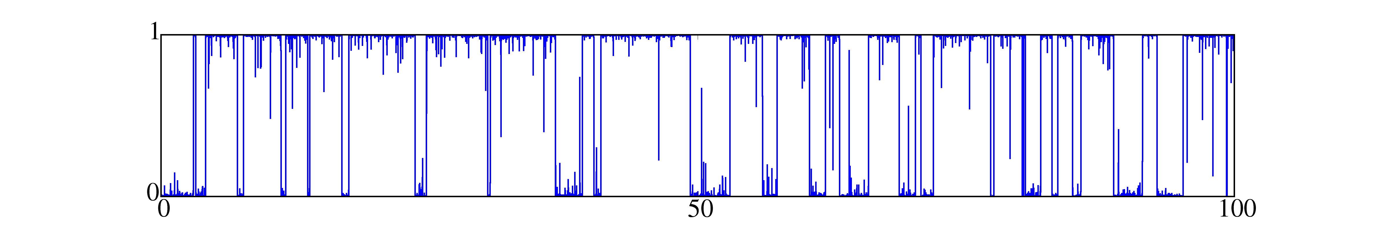
Figure 1: Thermally activated quantum jumps: A sample realisation for $p=.6$, $\tau_{\rm therm}=1$,and $\tau_{\rm meas}=10^{-6}$ of the $Q_{t}$ trajectories for a Q-bit in contact with a thermal bath and under continuous energy measurement. Note the structure of the unsuccessful excursions in between jumps.

A sample solution of the discrete version of (4) is shown in Fig.1. It clearly exhibits thermally activated quantum jumps between the two energy eigen-states. The aim of the following is to give a description of the dynamics and statistics of these jumps. They arise from the competitive contributions of the evolution and the continuous measurement. Their statistics will be derived by analysing the random quantum trajectories (4) of $Q$. They resemble Kramer’s like transitions but not quite because we are dealing with $\gamma^{2}\gg\lambda$ which is not the usual small noise limit [30, 31]. However, (4) shows that the noise becomes negligible for $Q$ close to $0$ (precisely $Q\ll\sigma^{1/2}$) or close to $1$, and this is the reason why the small $\sigma$ limit is manageable. Below we describe the invariant measure for (4), the waiting time and transition time statistics of (4).

Before entering into the detailed description, let us deal with a question of interpretation. Density matrices code for ensemble averages, i.e. they define measures (in the sense of probability) to compute expectations of system observables when experiments are repeated under identical conditions, say identical quantum systems in contact with reservoirs. When implementing Von Neumann measurements on the probes, we are still working with ensemble averages for the system plus reservoir even though we have got specific outputs for these measurements. The meaning of the quantum trajectories (4) is that they code for the measure (in the sense of probability) for system observables conditioned on having got some given outputs for the probe measurements (that is, a measure on ensemble of systems identically prepared and all having got these probe outputs). Furthermore, any given specific realisation of the system plus reservoir evolution is unitary (and this is the point of view associated to quantum stochastic differential equation [32]) but the reservoir is macroscopic and usually not observed nor controlled. What is expected, and usually assumed, is that there is some kind of concentration of measure so that there is no relevant rare event. And hence, predictions based on using density matrices to compute (conditional) ensemble averages are believed, or expected, to faithfully represent typical behaviours as well as the mean behaviour.

3 Statistics of jumps

We now present results on the statistics of jumps, including properties of the invariant measure and its behaviour when $\sigma\to 0$, a description of the statistics of the jump process especially in the limit $\sigma\to 0$. We choose to organise the presentation by first giving a – somewhat informal – description of these properties and then elements of proof – including more precise statements.

The invariant measure.
The quantum trajectories (4) admit an invariant measure (in the sense of probability) which possesses two peaks respectively centred close to $0$ and $1$ (more precisely around $Q_{-}\simeq p\sigma$ and $Q_{+}\simeq 1-(1-p)\sigma$). It slightly differs from the expected Gibbs measure for $\sigma$ finite ($\sigma:=2\tau_{\rm meas}/\tau_{\rm therm}$), but it converges in the limit of vanishing $\sigma$ (i.e. for a vanishingly small measurement time),

$$\lim_{\sigma\to 0}dP_{\rm stat}=\big{(}(1-p)\delta(Q)+p\delta(Q-1)\big{)}dQ.$$ (5)

For such a simple system, any initial measure converges to the stationary measure in the long run, so that $\lim_{t\to\infty}\mathbb{E}[F(Q_{t})]=\mathbb{E}_{\rm stat}[F(Q)]$ for any reasonable function $F$. In particular $\mathbb{E}_{\rm stat}[Q]=p$ and $\lim_{t\to\infty}\mathbb{E}[\rho_{t}]=p\,|0\rangle\langle 0|+(1-p)\,|1\rangle\langle 1|$ is the Gibbs state $\propto e^{-\beta H_{\rm sys}}$. In absence of measurements, the thermalization time scale is $\tau_{\rm therm}=\lambda^{-1}$. For instance $\mathbb{E}[(p-Q_{t})]=(p-Q_{0})e^{-\lambda t}$. We prove that this relaxation time is unmodified by the measurement process, $\lim_{\sigma\to 0}\,\tau_{\rm relax}=\lambda^{-1}$.

Sketch of the proof: Let us write (4) in the form $dQ_{t}=\gamma^{2}\,f(Q_{t})dt+\gamma\,g(Q_{t})dB_{t}$ and define a function $h(Q)$ by $\partial_{Q}h(Q)=-f(Q)/g^{2}(Q)$. By a classical result (see e.g. [35]) the invariant measure reads $dP_{\rm stat}=g^{-2}(Q)\,e^{-2h(Q)}\,dQ$. Explicitely,

$$dP_{\rm stat}=\frac{1}{Z_{\sigma}}\,\frac{dQ}{Q^{2-a_{\sigma}}(1-Q)^{2+a_{\sigma}}}\,\exp\big{[}-{\sigma}\big{(}\frac{p}{Q}+\frac{1-p}{1-Q}\big{)}\big{]}.$$

with $Z_{\sigma}$ a normalisation factor and $a_{\sigma}:=\sigma({2p-1})$. We infer that the density $dP_{\rm stat}/dQ$ exhibits two peaks at $0<Q_{-}<Q_{+}<1$ and a minimum in between, with $Q_{-}\simeq p\sigma$, and $1-Q_{+}\simeq(1-p)\sigma$ for $\sigma\ll 1$.

It is instructive to change variables, bringing (4) in a standard normalized form. The process $X_{t}:=\log(\frac{Q_{t}}{1-Q_{t}})$ takes value on the real axis since $0<Q_{t}<1$. Using Itô’s formula, (4) becomes $dX_{t}=-\gamma^{2}\,V^{\prime}(X_{t})\,dt+\gamma\,dB_{t}$ with effective double-well potential

$$V(X)=\frac{1}{2}(1-a_{\sigma})\log Q+\frac{1}{2}(1+a_{\sigma})\log(1-Q)+\frac{\sigma}{2}\big{[}\frac{p}{Q}+\frac{1-p}{1-Q}\big{]}.$$

The height of the barrier is logarithmic in $\sigma$. The invariant measure reads $dP_{\rm stat}\propto e^{-2V(X)}\,dX$.

Eq.(5) may be proved by computing the weight of $dP_{\rm stat}$ on the interval $[0,\alpha]$ for $0<\alpha<1$, that is $\int_{0}^{\alpha}dP_{\rm stat}$ when $\sigma\to 0$. For $\sigma$ small and $Q$ close to $0$, we may set $\sigma=0$ except in the exponential term $(\frac{\sigma p}{Q})$ so that

$$\int_{0}^{\alpha}dP_{\rm stat}\underset{\sigma\to 0}{\sim}\frac{1}{Z_{\sigma}}\int_{0}^{\alpha}\frac{dQ}{Q^{2}}e^{-\sigma p/Q}\underset{\sigma\to 0}{\sim}\frac{1}{Z_{\sigma}}(\frac{1}{\sigma p}).$$

The crucial point is that this dominant contribution is $\alpha$-independent. Similarly, computing the weight of the measure on $[1-\alpha,1]$, we get $\int_{1-\alpha}^{1}dP_{\rm stat}\,\underset{\sigma\to 0}{\sim}{1}/{(Z_{\sigma}\sigma}(1-p))$ which is also $\alpha$-independent. This means that in the limit $\sigma\to 0$ all the weight is concentrated at $0$ and $1$. The relative weight of the two peaks is $(1-p)/p$ and this proves (5).

For $\sigma$ small we get the following estimates, approximating the Dirac point measures

$$dP_{\rm stat}\underset{\sigma\to 0}{\sim}\begin{cases}\sigma p(1-p)\,Q^{-2}dQ\,\exp{(-{\sigma}\frac{p}{Q})}&{\rm for}\ Q\to 0,\\ ~{}&{}\textstyle\\ \sigma p(1-p)\,(1-Q)^{-2}dQ\,\exp{(-{\sigma}\frac{1-p}{1-Q})},&{\rm for}\ Q\to 1.\end{cases}$$

The approach to the invariant measure is governed by the Fokker-Planck operator ${\cal H}_{\rm HP}$ associated to (4), and more precisely by its first non zero eigen-value. As usual, this operator is not symmetric but it is self-transposed up to a conjugation, ${\cal H}_{\rm FP}^{T}=e^{-2V}\,{\cal H}_{\rm FP}\,e^{+2V}$. The operator ${\cal H}_{\rm FP}^{T}$ is the operator which codes for the evolution of expectations, that is $d\mathbb{E}[F(Q_{t})]=\mathbb{E}[({\cal H}_{\rm FP}^{T}\cdot F)(Q_{t})]dt$ for any function $F$. We know two eigen-functions of ${\cal H}_{\rm FP}^{T}$ which are $1$ and $p-Q$ with respective eigen-value $0$ and $-\lambda$, because $\mathbb{E}[p-Q_{t}]=(p-Q_{0})e^{-\lambda t}$. Hence we know two eigen-vectors of ${\cal H}_{\rm FP}$: the stationary measure $P_{\rm stat}\propto e^{-2V}$ with zero eigen-value and $P_{1}\propto(p-Q)\,e^{-2V}$ with eigen-value $-\lambda$. These are the two first eigen-values because $P_{\rm stat}$ has no zero and $P_{1}$ a unique zero. Hence $\tau_{\rm relax}=\lambda^{-1}$, and the relaxation time is not modified by the measurement process.

The statistics of waiting times and jumps.
This concerns the statistics of the time spent by the quantum trajectories near the value $Q_{-}\simeq 0$ and $Q_{+}\simeq 1$ respectively, so that the Q-bit is effectively close to the state $|1\rangle$ or $|0\rangle$. We prove that the limits of the mean time $T_{0}$ (resp. $T_{1}$) the quantum trajectories spend near the state $|0\rangle$ (resp. $|1\rangle$) are

$$\lim_{\sigma\to 0}\,T_{0}=\tau_{\rm therm}/(1-p),\quad\lim_{\sigma\to 0}\,T_{1}=\tau_{\rm therm}/p,$$ (6)

so that $\lim_{\sigma\to 0}\,T_{1}/T_{0}=e^{-\beta\omega}$ as expected from ergodicity. Contrary to the zero temperature quantum jumps, the mean waiting times of the thermally activated jumps stay finite when the measurement time decreases, as they should. The precise distribution is determined below in the limit of $\sigma\to 0$, see eq.(8): starting at $Q_{i}$, the distribution of the first passage time at $Q_{f}$ ($0\leq Q_{i}<Q_{f}\leq 1$) is a mixture of a Dirac peak at $0$ and an exponential distribution whose parameter depends on $Q_{f}$. For $Q_{i}=0$ the distribution is purely exponential. The succession of passage times at $0$ and $1$ is thus kind of (and exactly for $p=1/2$) a Poisson point process.

Sketch of the proof: We define these waiting times as the times needed to transit from one potential minimum to the other. To be specific we define $T_{1}$ (resp. $T_{0}$) as the first instance the quantum trajectory $Q_{t}$, starting at $Q_{i}$ close to $0^{+}$ (resp. $1^{-}$) reaches $Q_{f}$ close to $1^{-}$ (resp. $0^{+}$). These are stopping times, and to compute their mean is a standard problem in stochastic differential equations, see e.g. [33, 34]. Let us write (4) in the form $dQ_{t}=\gamma^{2}\,f(Q_{t})dt+\gamma\,g(Q_{t})dB_{t}$ and define a function $h(Q)$ by $\partial_{Q}h(Q)=-f(Q)/g^{2}(Q)$, so that the invariant measure reads $dP_{\rm stat}=g^{-2}(Q)\,e^{-2h(Q)}\,dQ$. By a classical formula, the mean time spend around $Q_{i}$ (close to the left minimum of the potential) is then

$$T_{1}=2\gamma^{-2}\int_{Q_{i}}^{Q_{f}}dQ\,e^{2h(Q)}\int_{0}^{Q}dP_{\rm stat}.$$

This formula is in fact a limiting formula for the time to leave an interval : in our case, the interval is $[0,Q_{f}]$ and the singularity at $0$ ensures that the exit is always at $Q_{f}$. This explains the presence of $0$ as the lower bound in the integral over $dP_{\rm stat}$. We do this integral as above when proving convergence of the stationary measure and approximate $e^{2h(Q)}$ by $e^{\sigma p/Q}$ for $\sigma$ small enough. This yields

$$T_{1}\underset{\sigma\to 0}{\sim}2\gamma^{-2}\int_{Q_{i}}^{Q_{f}}dQ\,e^{\sigma p/Q}\int_{0}^{Q}\frac{dQ^{\prime}}{Q^{\prime 2}}e^{-\sigma{p}/{Q^{\prime}}}\underset{\sigma\to 0}{\sim}\frac{2(Q_{f}-Q_{i})}{\sigma\gamma^{2}}\frac{1}{p}.$$

This formula is valid for any $Q_{i}<Q_{f}$, and quantum jumps correspond to $Q_{i}\simeq 0$ and $Q_{f}\simeq 1$, leading to $T_{1}\underset{\sigma\to 0}{\sim}\frac{2}{\sigma\gamma^{2}}\frac{1}{p}$ for $\sigma$ small. The mean time $T_{0}$ spend around $Q_{+}\simeq 1$ is simply obtained from the previous integral with $p\to 1-p$. Recall that $\sigma=2\tau_{\rm meas}/\tau_{\rm therm}$ and $\tau_{\rm meas}=\gamma^{-2}$. This proves (6).

To deal with the full distribution of waiting times, we observe that, by the strong Markov property, we have

$${\mathbb{E}}[e^{-uT_{i\to f}/\tau_{\text{therm}}}]=e^{-\int_{Q_{i}}^{Q_{f}}\varphi(Q,u)dQ}.$$ (7)

for some function $\varphi(Q,u)$, where $T_{i\to f}$ is by definition the random time it takes to go from $Q_{i}$ to $Q_{f}>Q_{i}$, so $T_{i\to f}$ is a stopping time. We use a standard martingale trick (see e.g. chapter 7 [34]): by construction the conditional expectation $N_{t}:={\mathbb{E}}[e^{-uT_{i\to f}/\tau_{\text{therm}}}|\mathcal{F}_{t}]$ is a martingale. On the other hand, by the Markov property, $N_{t}=e^{-ut/\tau_{\text{therm}}}e^{-\int_{Q_{t}}^{Q_{f}}\varphi(Q,u)dQ}$. Itô’s formula applied to $N_{t}$ yields that

$$\sigma\big{(}-u+(p-Q)\varphi\big{)}+Q^{2}(1-Q)^{2}\big{(}\varphi^{\prime}+\varphi^{2}\big{)}=0,$$

where $\varphi^{\prime}$ is the derivative of $\varphi$ with respect to $Q$. The shortest route to take the $\sigma\to 0$ limit is as follows. For $\sigma=0$ the equation degenerates to $\varphi^{\prime}+\varphi^{2}=0$, so that in this limit $\varphi(Q,u)=\frac{\varphi_{0}(u)}{1+Q\varphi_{0}(u)}$ for some integration “constant” $\varphi_{0}(u)$. For small $Q$ the noise becomes irrelevant, so that $T_{i\to f}$ becomes deterministic when both $Q_{i}$ and $Q_{f}$ are close to $0$. In this regime, (4) degenerates to $dQ_{t}=\lambda pdt$, a motion at constant speed. This gives $\varphi_{0}(u)=u/p$, and $\varphi(Q,u)=\frac{u}{p+uQ}$. Finally, in the limit $\sigma\to 0$

$$\lim_{\sigma\to 0}\,{\mathbb{E}}[e^{-uT_{i\to f}/\tau_{\text{therm}}}]=\frac{uQ_{i}+p}{uQ_{f}+p}.$$

Undoing the Laplace transform, we obtain that, for any Borel subset $B$ in $\mathbb{R}$,

$$\lim_{\sigma\to 0}\,{\mathbb{P}}[T_{i\to f}/\tau_{\text{therm}}\in B]=\frac{Q_{i}}{Q_{f}}\,{\mathbb{I}}_{\,0\in B}+\Big{(}1-\frac{Q_{i}}{Q_{f}}\Big{)}\frac{p}{Q_{f}}\int_{B}e^{-s\frac{p}{Q_{f}}}ds,$$ (8)

i.e. the law of $T_{i\to f}$ is a mixture of a Dirac peak at $0$ (weight $Q_{i}/Q_{f}$) and an exponential distribution of parameter $\frac{p}{Q_{f}}$ (weight $1-Q_{i}/Q_{f}$). Intuitively when $\sigma\to 0$ but $Q_{i}>0$ the trajectory starting at $Q_{i}$ has a chance to reach $Q_{f}$ without being trapped in the potential well, hence the presence of a Dirac peak. However if $Q_{i}\lesssim\sigma\to 0$, the trajectory has to go through the potential well and waits there an exponential time. The $Q_{f}$-dependence of this exponential time, already visible in the mean waiting time, shows that the situation is not exactly covered by standard Kramer’s arguments, i.e. it is not only the escape from a potential well that counts. In the $Q$-coordinate, this is interpreted as a multiplicative noise effect: when $Q(1-Q)$ departs significantly from $0$, the noise becomes very large (a look at Fig.1 and its many spikes may be illuminating at that point). In this $X$-coordinate, this is interpreted as the fact that the potential wells are only logarithmically deep, and their separation is very large.

The transition time statistics.
To get a clue on the jump dynamics let us now look at the mean time needed to transit between the two energy eigen-states. These are independent of the direction of the transition, either from $Q\simeq 0$ to $Q\simeq 1$ or the reverse. We shall prove that they are determined by the measurement time up to logarithmic corrections (which may be large),

$$\tilde{\tau}\ \underset{\sigma\to 0}{\sim}\ 4\,\tau_{\rm meas}\ \log(\tau_{\rm therm}/\tau_{\rm meas}).$$ (9)

This shows that the inside jump dynamics is dominated by the measurement procedure but also influenced by the other dynamical processes which are the sources of the fluctuations.

Sketch of the proof: The transition time is the time it takes to cross the barrier in events where this is really what happens: the process is to start at one point $Q_{i}$ (on one side of the barrier) and leave it for good until it reaches a point $Q_{f}$ (on the other side of the barrier). This means we want to make statistics only on certain events, i.e. we have to condition. If $Q_{i}$ is not a singular point for the diffusion, a typical sample starting at $Q_{i}$ will, with probability $1$, visit $Q_{i}$ again uncountably many times in an arbitrary small time interval. This means that some limiting procedure is needed to define conditioning: one starts the process at an intermediate point $Q$ between $Q_{i}$ and $Q_{f}$ and conditions on the event that $Q_{f}$ is reached before $Q_{i}$, then the limit $Q\to Q_{i}$ is taken. As we shall recall below, the equation for the conditioned process does not depend on $Q_{f}$, but for the conditioned process the point $Q_{i}$ is singular, so that even if the conditioned process is started at $Q_{i}$, $Q_{i}$ is immediately left for good.

We begin by recalling some general formulæ. A general reference completing [33, 34] for this discussion is [35]. If $dQ_{t}=\gamma^{2}f(Q_{t})dt+\gamma g(Q_{t})dB_{t}$ is the diffusion equation describing the time evolution of $Q_{t}$, we define the so-called scale function $s(Q)$ by $s^{\prime\prime}/s^{\prime}=-2f/g^{2}$. From the definition, the scale function is defined modulo an affine transformation. The scale function is related to the previously introduced function $h$ by the simple relation $s^{\prime}(Q)\propto e^{2h(Q)}$ but for the purpose of the present discussion, $s$ is slightly more convenient. Itô’s formula shows that $s(Q_{t})$ is a continuous (local) martingale, i.e. a time-changed Brownian motion. A classical result, easily retrieved by standard martingale techniques for instance, is that $\Pi_{[Q_{i},Q_{f}]}(Q)$, the probability starting at $Q\in[Q_{i},Q_{f}]$ to exit the interval at $Q_{f}$ is

$$\Pi_{[Q_{i},Q_{f}]}(Q)=\frac{s(Q)-s(Q_{i})}{s(Q_{f})-s(Q_{i})}.$$

In fact, this is the origin of the scaling function: if $s(Q)$ is used as a new “space” variable, exit probabilities look like those of Brownian motion. This is to be expected because exit probabilities do not involve a time parameterisation, so they are the same for Brownian motion and time-changed Brownian motion. The probability $\Pi_{[Q_{i},Q_{f}]}(Q)$, abbreviated as $\Pi(Q)$ in the sequel, is relevant because we want to condition precisely on those samples that contribute to it. This is achieved by a Girsanov transformation: Girsanov’s theorem states that the equation governing the initial motion conditioned to exit $[Q_{i},Q_{f}]$ at $Q_{f}$ is $dQ_{t}=\gamma^{2}\tilde{f}(Q_{t})dt+\gamma g(Q_{t})d\tilde{B}_{t}$ where $\tilde{B}_{t}$ is a Brownian motion and $\tilde{f}:=f+g^{2}\frac{\Pi^{\prime}}{\Pi}$. To say things in a different but equivalent way: under conditioning, the process $B_{t}$ is not a Brownian motion anymore, but $\tilde{B}_{t}:=B_{t}-\gamma\int_{0}^{t}g^{2}(Q_{s})\frac{\Pi^{\prime}(Q_{s})}{\Pi(Q_{s})}ds$ becomes one. Note that $Q_{f}$ does not appear in $\frac{\Pi^{\prime}(Q)}{\Pi(Q)}=\frac{s^{\prime}(Q)}{s(Q)-s(Q_{i})}$ which has a simple pole with residue $1$ at $Q=Q_{i}$, a singularity characteristic of conditioning not to pass at $Q_{i}$. This singularity implies that the transition time $\tilde{\tau}$ can be written as a double integral: defining $\tilde{h}$ (the analogue of $h$ but for the conditioned equation) by $\tilde{h}^{\prime}:=-\tilde{f}/g^{2}$, we get

$$\tilde{\tau}=2\gamma^{-2}\int_{Q_{i}}^{Q_{f}}dQ\,e^{2\tilde{h}(Q)}\int_{Q_{i}}^{Q}dq\,e^{-2\tilde{h}(q)}/g(q)^{2}.$$

Note that in the inner integral the lower bound is again the position of repelling singularity, i.e. $Q_{i}$ for the conditioned equation, just as it was $0$ for the initial equation. Re-expressing $\tilde{h}$ in terms of the scale function, the fact that the singularity comes from conditioning leads to further simplifications via integrations by part, leading finally to

$$\tilde{\tau}=\frac{2\gamma^{-2}}{s(Q_{f})-s(Q_{i})}\int_{Q_{i}}^{Q_{f}}dQ\frac{\big{(}s(Q)-s(Q_{i})\big{)}\big{(}s(Q_{f})-s(Q)\big{)}}{s^{\prime}(Q)g^{2}(Q)}.$$

These are general formulæ that we gave because the tricks are simpler to disentangle in the general setting. It is reassuring to observe that the results for the exit probabilities or for the transition time are indeed invariant under affine transformations of the scale function.

In the case at hand, $f(Q)=\sigma(p-Q)/2$ and $g(Q)=Q(1-Q)$ leading to the formula $s^{\prime}(q)=\left(\frac{1-q}{q}\right)^{\sigma(2p-1)}e^{\sigma(\frac{p}{q}+\frac{1-p}{1-q})}$. In the limit when $\sigma\to 0$ for $Q$ staying in a $\sigma$ independant interval, $s(Q)$ becomes an affine function of $Q$, so that for fixed $Q_{i}$ and $Q_{f}$, the mean transition time $\tilde{\tau}$ is given by the integral $2\gamma^{-2}\int_{Q_{i}}^{Q_{f}}\frac{dQ}{g^{2}(Q)}\frac{(Q-Q_{i})(Q_{f}-Q)}{(Q_{f}-Q_{i})}$, and we get

$$\tilde{\tau}\underset{\sigma\to 0}{\sim}\frac{2}{\gamma^{2}}\Big{(}\frac{Q_{i}+Q_{f}-2Q_{i}Q_{f}}{Q_{f}-Q_{i}}\log\frac{Q_{f}(1-Q_{i})}{Q_{i}(1-Q_{f})}-2\Big{)}.$$

Note that this formula is $p$-independent.

Up to now, we have taken $Q_{i}$ and $Q_{f}$ fixed and taken the limit $\sigma\to 0$. What we really want is more subtle, because we want $Q_{i}$ and $Q_{f}$ to sit at the bottoms of the potential wells, which are $\sigma$-dependent. The trouble is that near the bottoms, the scale function $s(Q)$ is not well-described by an affine function. Ignoring this problem for a while, let us see what the naïve limiting approach “take the small $\sigma$ limit for fixed $Q_{i}$ and $Q_{f}$ and then take $Q_{i}$ and $1-Q_{f}$ of order $\sigma$” predicts. Locating the positions of the bottoms of the potential wells for small $\sigma$, we get $Q_{i}\simeq p\sigma$ and $Q_{f}\simeq 1-(1-p)\sigma$. Plugging these asymptotics blindly in the above formula for $\tilde{\tau}$ we get, for the transition time from one potential well to the other in the small $\sigma$ limit,

$$\tilde{\tau}\underset{\sigma\to 0}{\sim}-\frac{4}{\gamma^{2}}\log\sigma\underset{\sigma\to 0}{\sim}4\,\tau_{\rm meas}\log(\tau_{\rm therm}/\tau_{\rm meas})$$

as announced above. The rigorous justification of this formula, taking properly into account the region where the affine approximation for $s(Q)$ fails, requires some effort. The details are given in Appendix A using an argument suggested to us by an anonymous referee, see especially eq.(11). There is no dependence in $p$ in the expression for $\tilde{\tau}$, but it is valid only for $\sigma\ll p(1-p)$.

4 Non-sensitivity to initial conditions

This very short section is less rigorous than the previous ones. We give a heuristic argument that for given probe measurement outcomes (i.e. for a given realisation of the Brownian motion), two trajectories with different initial conditions get closer at an exponential rate on a time scale of order $\tau_{\rm meas}$. This means that there is exponential memory loss. This generalises in the presence of thermal noise the result of [25] on repeated non-demolition measurements.

The stochastic differential equation (4) only involves smooth driving functions and the solutions of interest remain bounded in $[0,1]$. Thus its solutions behave “nicely”: two solutions with different initial conditions $0\leq Q_{0}<Q^{\prime}_{0}\leq 1$ but for the same sample of Brownian motion cannot stick together at any later time (i.e. strong existence and uniqueness of the solution for a given realisation of the Brownian motion hold). As trajectories are continuous, this means that $Q_{t}<Q^{\prime}_{t}$ for every $t$. For $\sigma$ small enough, this implies that these two solutions cannot avoid getting very close because both $Q_{t}$ and $Q^{\prime}_{t}$ have to jump between values close to $0$ and $1$. Once they are close, we can accurately linearise (4) around the solution $Q_{t}$.

Linear theory.
Keeping only first order terms in the deviation $\Delta_{t}:=Q^{\prime}_{t}-Q_{t}$, we get from (4)

$$d\Delta_{t}=[-\lambda\,dt+\gamma\,(1-2Q_{t})\,dB_{t}]\Delta_{t}.$$ (10)

We claim that any solution $\Delta_{t}$ of (10) with positive initial condition stays positive forever and converges almost surely to $0$. The convergence is exponential, and for small $\sigma$ the rate is twice the typical measurement time $\tau_{\rm meas}=\gamma^{-2}$. Moreover $\Delta_{t}$ is a super-martingale.

Sketch of the proof: We define $M_{t}$ by writing $\Delta_{t}=:\Delta_{0}e^{-\lambda\,t}M_{t}$. Then $M_{0}=1$ and $dM_{t}=\gamma\,M_{t}(1-2Q_{t})\,dB_{t}$. So $M_{t}$ is a local martingale, and Itô’s formula yields immediately that

$$M_{t}=\exp\left(-\frac{\gamma^{2}}{2}\int_{0}^{t}(1-2Q_{s})^{2}\,ds+\gamma\int_{0}^{t}(1-2Q_{s})\,dB_{s}\right).$$

As $Q_{s}\in[0,1]$ for all $s$, the Riemann and Itô integrals on the right-hand side are finite for every $t$ for almost every sample. Moreover, the bound $e^{\frac{\gamma^{2}}{2}\int_{0}^{t}(1-2Q_{s})^{2}\,ds}\leq e^{\frac{\gamma^{2}}{2}\,s}$ implies that $M_{t}$ satisfies the Novikov criterion (see e.g. [33, 34]), hence that $M_{t}$ is well-defined, positive for every $t$, and is a martingale. Consequently, if $\Delta_{0}>0$, $\Delta_{t}$ is a super-martingale. A naïve scaling argument indicates that $\int_{0}^{t}(1-2Q_{s})^{2}\,ds$ scales like $t$ for large $t$ whereas $\int_{0}^{t}(1-2Q_{s})\,dB_{s}$ scales like $\sqrt{t}$, so that $\lim_{t\to+\infty}M_{t}=0$ almost surely, and thus $\lim_{t\to+\infty}\Delta_{t}=0$ almost surely as well. One can be a bit more precise. For large $\gamma$ (i.e. $\sigma$ small) the trajectory $Q_{s}$ spends most of its time close to $0$ or $1$. Actually, most of the time $Q_{s}\propto\sigma$ or $1-Q_{s}\propto\sigma$, so that $(1-2Q_{s})^{2}-1=-4Q_{s}(1-Q_{s})$ is most of the time of order $\sim\sigma$. We infer that $\log M_{t}=-\frac{\gamma^{2}}{2}t+\gamma\tilde{B}_{t}+O(1)$ for large $\gamma$, where $\tilde{B}_{t}:=\int_{0}^{t}\text{sign}(1-2Q_{s})\,dB_{s}$ is a standard Brownian motion. In particular, the rate at which trajectories corresponding to different initial conditions but the same measurement outcomes approach each other is twice the typical measurement time $\tau_{\rm meas}=\gamma^{-2}$ for large $\gamma$.

5 Generalisations and outlook.

The above study can be generalised to a system in contact with thermal reservoirs and under continuous time measurement with higher dimensional Hilbert spaces both for the system and for the probes. Let us briefly present the general picture. As above we can restrict ourselves to diagonal density matrices if the Hamiltonian and thermal Lindbladian flows commute. Let

$$\rho=\sum_{\alpha}Q_{\alpha}\ |\alpha\rangle\langle\alpha|,\quad\sum_{\alpha}Q_{\alpha}=1,$$

be the system density matrix, diagonal in the energy eigen-state basis. The time evolution of its components is going to be the sum of the thermal and noisy evolutions, induced by the measurement,

$$dQ_{\alpha}=(dQ_{\alpha})_{\rm therm}+(dQ_{\alpha})_{\rm meas}.$$

As before, we may model the thermal evolution by a Lindbladian [27]. That is $(d\rho)_{\rm therm}=L_{\rm therm}(\rho)\,dt$, with $L_{\rm therm}(\rho)=\sum_{a}\big{[}C_{a}\rho\,C^{\dagger}_{a}-\frac{1}{2}\{C^{\dagger}_{a}C_{a},\rho\}\big{]},$ for some operators $C_{a}$ acting on ${\cal H}_{s}$. When projected on diagonal density matrices, this becomes

$$(dQ_{\alpha})_{\rm therm}=\sum_{\gamma}\big{(}L_{\alpha\gamma}-\ell_{\alpha}\,\delta_{\alpha;\gamma}\big{)}Q_{\gamma}\,dt,$$

with $L_{\alpha\gamma}:=\sum_{a}|\langle\alpha|C_{a}|\gamma\rangle|^{2}$ and $\ell_{\alpha}:=\sum_{a}\langle\alpha|C^{\dagger}_{a}C_{a}|\alpha\rangle$. The matrix $L$ is real but (a priori) not symmetric and $\sum_{\alpha}L_{\alpha\gamma}=\ell_{\gamma}$ as it should be by compatibility with $\sum_{\alpha}Q_{\alpha}=1$. Demanding that the Gibbs state is a steady state imposes $\sum_{\gamma}L_{\alpha\gamma}p_{\gamma}=\ell_{\alpha}\,p_{\alpha}$, where $p_{\alpha}=e^{-\beta_{\alpha}}/(\sum_{\gamma}e^{-\beta_{\gamma}})$ is the Boltzmann weight. To rephrase these observations: the matrix $L_{\alpha\gamma}-\ell_{\alpha}\,\delta_{\alpha;\gamma}$ describing the thermal evolution is the infinitesimal generator of a finite state continuous time Markov process, to which all standard results of probability theory apply.

The evolution equations for continuous time energy measurement have been described in [16, 17]. We borrow the notations from [29] which deals with the simpler non-demolition case. Let us index by $i$, from $1$ to ${\rm dim}{\cal H}_{p}$, the probe measurement outputs. In the diffusive case, these equations reads $(dQ_{\alpha})_{\rm meas}=Q_{\alpha}\sum_{i}[\Gamma(i|\alpha)-\langle{\Gamma(i)}\rangle]dB_{i}$, with $B_{i}$ Brownian motions, $\sum_{i}B_{i}=0$, with quadratic variation $dB_{i}dB_{j}=[\delta^{ij}p_{0}(i)-p_{0}(j)p_{0}(j)]dt$ where the $p_{0}(i)$’s are probabilities on the set of probe measurement outputs, $\sum_{i}p_{0}(i)=1$. Here $\Gamma(i|\alpha)$ are parameters coding for the interaction involved in weak measurements, $\sum_{i}p_{0}(i)\Gamma(i|\alpha)=0$, and $\langle\Gamma(i)\rangle=\sum_{\alpha}\Gamma(i|\alpha)Q_{\alpha}$. Defining $dW_{\alpha}:=\sum_{i}\Gamma(i|\alpha)dB_{i}$, these equations becomes

$$(dQ_{\alpha})_{\rm meas}=Q_{\alpha}\big{[}dW_{\alpha}-(\sum_{\gamma}Q_{\gamma}dW_{\gamma})\big{]},\quad{\rm with}\ dW_{\alpha}\,dW_{\beta}=\bar{\Gamma}_{\alpha\beta}\,dt,$$

where $\bar{\Gamma}_{\alpha\beta}=\sum_{j}p_{0}(j)\Gamma(j|\alpha)\Gamma(j|\beta)$. It is compatible with $\sum_{\alpha}Q_{\alpha}=1$.

Two special cases are of particular interest: (a) the probe Hilbert space is of dimension $2$ as above, there is then only one Brownian motion involved – because the measurement outputs are in one-to-one correspondence with random walks – and we may write $dW_{\alpha}=\gamma_{\alpha}dB_{t}$ for some parameters $\gamma_{\alpha}$; and (b) the dimension of the probe Hilbert space is larger than that of the system Hilbert space so that all Brownian motions $W_{\alpha}$ are independent. In both cases we are actually dealing with particular random processes on probability measures.

These cases will be analysed in [36], but the general picture is clear. The invariant measure is going to be localised around unstable ‘fixed’ points, $Q_{\alpha}\simeq\delta_{\alpha;\gamma}+{\rm corrections}$, in one-to-one correspondence with the energy eigen-states. Any given quantum trajectory is going to wait long periods of time around these points but jump randomly from time to time to another basin of attraction. They hence yield a fuzzy trajectory realisation of the thermal Markov chain. The waiting times are encoded in the thermal Lindbladian, which here reduces to the Markov matrix $(L_{\alpha\gamma}-\ell_{\alpha}\delta_{\alpha;\gamma})$. Indeed, using a frequency interpretation of the $Q$’s, the off-diagonal elements of $L_{\alpha\gamma}$ codes for a transfer of population from state $\gamma$ to state $\alpha$, and the natural time associated to transfer from state $\gamma$ to any other states is $T_{\gamma}$ with $T_{\gamma}^{-1}:=\sum_{\alpha\not=\gamma}L_{\alpha\gamma}$. The transition times are going to be determined by the time scale involved in the measurement process, up to logarithmic corrections. In the discrete framework these are given by relevant relative entropies [25] and are therefore asymmetric (i.e. the collapse rate of $Q_{\gamma}$ while converging to state $\alpha$ is different from the collapse rate of $Q_{\alpha}$ while converging to $\gamma$). In the continuous time limit these rates become $\tau_{\alpha\gamma}$, with $\tau_{\alpha\gamma}^{-1}:=\frac{1}{2}\big{(}\bar{\Gamma}_{\alpha\alpha}-2\bar{\Gamma}_{\alpha\gamma}+\bar{\Gamma}_{\gamma\gamma}\big{)}$, and they are symmetric. These are naturally interpreted as the jumping times from state $\alpha$ to state $\gamma$, up to logarithmic corrections.

Finally, generalisations to out-of-equilibrium contexts, in which a system is in contact with different reservoirs at different temperatures, are particularly interesting. Describing quantum trajectory behaviours in such situations is a question we plan to address in [36].

Appendix A Details about the computation of $\tilde{\tau}$.

This Appendix is devoted to the proof that the approximate procedure we used to compute $\tilde{\tau}$ is correct. It is a slight elaboration of an argument provided to us by an anonymous referee.

For the rest of this appendix, we set $Q_{i}=p\sigma$ and $Q_{f}=1-(1-p)\sigma$ and define

$$l(Q):=\frac{\big{(}s(Q)-s(Q_{i})\big{)}\big{(}s(Q_{f})-s(Q)\big{)}}{s^{\prime}(Q)\big{(}s(Q_{f})-s(Q_{i})\big{)}},\quad l_{0}(Q):=\frac{(Q-Q_{i})(Q_{f}-Q_{i})}{(Q_{f}-Q_{i})}$$

and set

$$I[a,b]:=\int_{a}^{b}\frac{dQ}{g^{2}(Q)}l(Q),\quad I_{0}[a,b]:=\int_{a}^{b}\frac{dQ}{g^{2}(Q)}l_{0}(Q).$$

Recall that general arguments imply that the mean transition time from $Q_{i}$ to $Q_{f}$ is $\tilde{\tau}=2\gamma^{-2}I[Q_{i},Q_{f}]$. Our interest is in the asymptotics of $I[Q_{i},Q_{f}]$ in the limit $\sigma\to 0$. What we really did to estimate $\tilde{\tau}$ in the main text was some kind of inversion of limits: we computed the behaviour of $2\gamma^{-2}I_{0}[Q_{i},Q_{f}]$ when $\sigma\to 0$ (because for $Q$ in a $\sigma$-independent interval, $s(Q)$ becomes an affine function of $Q$ in the limit when $\sigma\to 0$).

Our aim is now to prove that the difference $I[Q_{i},Q_{f}]-I_{0}[Q_{i},Q_{f}]$ goes to a finite limit as $\sigma\to 0$.

To compare $I[Q_{i},Q_{f}]$ and $I_{0}[Q_{i},Q_{f}]$ in the limit $\sigma\to 0$ we introduce an auxiliary function $M(\sigma)$ such that $\lim_{\sigma\to 0}M(\sigma)=+\infty$ but $\lim_{\sigma\to 0}M(\sigma)\sigma\log\sigma=0$ and let $\hat{Q}_{i}:=p\sigma M(\sigma)$ and $\hat{Q}_{f}:=1-(1-p)\sigma M(\sigma)$. We split the integral

$$I[Q_{i},Q_{f}]=I[Q_{i},\hat{Q}_{i}]+I[\hat{Q}_{i},\hat{Q}_{f}]+I[\hat{Q}_{f},Q_{f}],$$

and similarly for $I_{0}$.

We first work on the intermediate integral, and then turn to the first (the third is analogous).

The integral $I[\hat{Q}_{i},\hat{Q}_{f}]$

We need some preliminary estimates. We define $d(Q,Q^{\prime}):=\frac{s(Q)-s(Q^{\prime})}{Q-Q^{\prime}}$.

Claims :
(a) There is a constant $K$ independant of $Q$ and $\sigma$ such that $|s^{\prime}(Q)|\leq K$ for $Q\in[Q_{i},Q_{f}]$. We write this as $s^{\prime}(Q)=O_{u}(1)$ for $Q\in[Q_{i},Q_{f}]$ . For $Q\in[\hat{Q}_{i},\hat{Q}_{f}]$, $s^{\prime}(Q)=1+O_{u}(1/M(\sigma))$
(b) For $Q\in[\hat{Q}_{i},\hat{Q}_{f}]$ one has $d(Q,Q_{i})=1+O_{u}(1/\sqrt{M(\sigma)})$ and $d(Q_{f},Q)=1+O_{u}(1/\sqrt{M(\sigma)})$.
(c) The ratio $\frac{s(Q_{f})-s(Q_{i})}{Q_{f}-Q_{i}}$ differs from $1$ by an $O_{u}(\sqrt{\sigma})$.
(d) The ratio $\frac{l(Q)}{l_{0}(Q)}$ differs from $1$ by an $O_{u}(\sqrt{\sigma})$.

Proof of (a): Recall that $s^{\prime}(Q)=e^{\sigma\left(\frac{p}{Q}+\frac{1-p}{1-Q}+(2p-1)\log\frac{1-Q}{Q}\right)}$. The derivative of the funtion in parenthesis is $\frac{Q-p}{g^{2}(Q)}$, so to get the uniform bound it suffices to compute $s^{\prime}(Q)$ at $Q=p$ and at the two boundaries. Now $s^{\prime}(p)=1+O_{u}(\sigma\log M(\sigma))$. Comparing to the boundary values leads to $s^{\prime}(Q)=O_{u}(1)$ for $Q\in[Q_{i},Q_{f}]$ and $s^{\prime}(Q)=1+O_{u}(1/M(\sigma))$ for $Q\in[\hat{Q}_{i},\hat{Q}_{f}]$.

Proof of (b): The trick is to introduce another function $N(\sigma)$ such that $\lim_{\sigma\to 0}N(\sigma)=+\infty$ but $N(\sigma)=o(M(\sigma))$. Let $\bar{Q}_{i}:=p\sigma N(\sigma)$ and write $s(Q)-s(Q_{i})=\left(s(Q)-s(\bar{Q}_{i})\right)+\left(s(\bar{Q}_{i})-s(Q_{i})\right)$. The intermediate value theorem ensures the existence of some $Q_{>}\in]\bar{Q}_{i},\hat{Q}_{f}[$ such that $s(Q)-s(\bar{Q}_{i})=(Q-\bar{Q}_{i})s^{\prime}(Q_{>})$ and some $Q_{<}\in]Q_{i},\bar{Q}_{i}[$ such that $s(\bar{Q}_{i})-s(Q_{i})=(\bar{Q}_{i}-Q_{i})s^{\prime}(Q_{<})$. Then

$$\frac{s(Q)-s(Q_{i})}{Q-Q_{i}}=s^{\prime}(Q_{>})+\frac{(\bar{Q}_{i}-Q_{i})}{Q-Q_{i}}(s^{\prime}(Q_{<})-s^{\prime}(Q_{>})).$$

Claim (a) but applied for $N$ instead of $M$ implies that the first term is $1+O_{u}(1/N(\sigma))$. Claim (a) again implies that $s^{\prime}(Q_{<})-s^{\prime}(Q_{>})=O_{u}(1)$. As $1/(Q-Q_{i})$ is maximal in the interval under consideration at $Q=\hat{Q}_{i}$ the second term is $O_{u}(N(\sigma)/M(\sigma))$. Balancing the two terms leads to choose $N(\sigma)\propto\sqrt{M(\sigma)}$, proving the claim. The second claim is proved analogously.

Proof of (c): The trick is to introduce a new auxiliary function $\tilde{N}(\sigma)$. This time we split $s(Q_{f})-s(Q_{i})$ in three pieces as $s(Q_{f})-s(1-(1-p)\sigma\tilde{N}(\sigma))+(s(1-(1-p)\sigma\tilde{N}(\sigma))-s(p\sigma\tilde{N}(\sigma)))+(s(p\sigma\tilde{N}(\sigma))-s(Q_{i}))$. The proof proceeds as the proof in the previous claim. This time the optimum is to choose $\tilde{N}(\sigma)\propto\sqrt{\sigma}$. We leave the details to the reader.

Proof of (d): Observe that

$$\frac{l(Q)}{l_{0}(Q)}=\frac{d(Q,Q_{i})d(Q_{f},Q)}{s^{\prime}(Q)d(Q_{f},Q_{i})}=1+O_{u}(1/\sqrt{M(\sigma)}).$$

All the factors are close to $1$ with deviations bounded, according to the previous claims, by $O_{u}(1/M(\sigma))$, $O_{u}(1/\sqrt{M(\sigma)})$ or $O_{u}(\sqrt{\sigma)})$. The softest one is $O_{u}(1/\sqrt{M(\sigma)})$, which proves the claim.

This leads to our first goal.

Claim:
The difference $I[\hat{Q}_{i},\hat{Q}_{f}]-I_{0}[\hat{Q}_{i},\hat{Q}_{f}]$ is $O(\frac{\log\sigma}{\sqrt{M(\sigma)}})$.

Proof: Recall that $I[\hat{Q}_{i},\hat{Q}_{f}]=\int_{\hat{Q}_{i}}^{\hat{Q}_{f}}\frac{dQ}{g^{2}(Q)}l(Q)$ (and the analog relating $I_{0}$ and $l_{0}(Q)$) so that we need to bound

$$\int_{\hat{Q}_{i}}^{\hat{Q}_{f}}\frac{dQ}{g^{2}(Q)}(l(Q)-l_{0}(Q))=\int_{\hat{Q}_{i}}^{\hat{Q}_{f}}\frac{dQ}{g^{2}(Q)}\left(\frac{l(Q)}{l_{0}(Q)}-1\right)l_{0}(Q).$$

By the previous claim, $\frac{l(Q)}{l_{0}(Q)}-1=O_{u}(1/\sqrt{M(\sigma)})$ which by uniformity can be taken outside the integral. The remaining integral is nothing but $I_{0}[\hat{Q}_{i},\hat{Q}_{f}]$ which we know is $\sim\log\sigma$, and the result follows.

The integral $I[Q_{i},\hat{Q}_{i}]$

Let $\mathfrak{M}>0$ be a constant. We start with the evaluation of some integrals, our main interest being their large $\mathfrak{M}$ behavior. The first observation is that:

$$J_{0}:=\int_{1}^{\mathfrak{M}}\frac{dY}{Y^{2}}(Y-1)=\log\mathfrak{M}-1+\frac{1}{\mathfrak{M}}=\log\mathfrak{M}-1+O(1/\mathfrak{M}).$$

Taking $Y=Q/Q_{i}$, we note that $\int_{Q_{i}}^{\hat{Q}_{i}}\frac{dQ}{Q^{2}}(Q-Q_{i})={J_{0}}_{|\mathfrak{M}=M(\sigma)}$.

Second we consider

$$J:=\int_{1}^{\mathfrak{M}}\frac{dY}{Y^{2}}\int_{1}^{Y}dy\,e^{1/y-1/Y},$$

which we expand at large $\mathfrak{M}$. Interchanging integrals

$$J=\int_{1}^{\mathfrak{M}}dy\int_{y}^{\mathfrak{M}}\frac{dY}{Y^{2}}e^{1/y-1/Y}=\int_{1}^{\mathfrak{M}}dy\left(e^{1/y-1/\mathfrak{M}}-1\right)=1-\mathfrak{M}+e^{-1/\mathfrak{M}}\int_{1}^{\mathfrak{M}}dy\,e^{1/y}.$$

Now using $e^{1/y}=\left(e^{1/y}-1-1/y\right)+\left(1+1/y\right)$ we get

$$\int_{1}^{\mathfrak{M}}dy\,e^{1/y}=\mathfrak{M}-1+\log\mathfrak{M}+\int_{1}^{\infty}dy\,\left(e^{1/y}-1-1/y\right)+O(1/\mathfrak{M}).$$

Setting $\mathfrak{I}:=\int_{1}^{\infty}dy\,\left(e^{1/y}-1-1/y\right)$, a straightforward expansion yields

$$J=-1+\mathfrak{I}+\log\mathfrak{M}-\frac{\log\mathfrak{M}}{\mathfrak{M}}+O(1/\mathfrak{M}).$$

In particular

$$J-J_{0}=\mathfrak{I}-\frac{\log\mathfrak{M}}{\mathfrak{M}}+O(1/\mathfrak{M})$$

We need some estimates again.

Claims :
(e) For $Q\in[Q_{i},\hat{Q}_{i}]$ we have $s(Q)-s(Q_{i})=O_{u}(\sigma M(\sigma))$.
(f) For $Q\in[Q_{i},\hat{Q}_{i}]$ we have $\frac{s(Q_{f})-s(Q)}{s(Q_{f})-s(Q_{i})}=1+O_{u}(\sigma M(\sigma))$.
(g) For $Q\in[Q_{i},\hat{Q}_{i}]$ we have $Q^{2}/g(Q)^{2}=1+O_{u}(\sigma M(\sigma)).$
(h) $I[Q_{i},\hat{Q}_{i}]=(1+O(\sigma M(\sigma)))J_{|\mathfrak{M}=M(\sigma)}$.

Proof of (e): We write $s(Q)-s(Q_{i})=(Q-Q_{i})s^{\prime}(Q_{<})$ for some $Q_{<}\in]Q_{i},\hat{Q}_{i}[$. Note that $|Q-Q_{i}|\leq\hat{Q}_{i}-Q_{i}=O_{u}(\sigma M(\sigma))$. By claim (a) $s^{\prime}(Q_{<})=O_{u}(1)$ because $[Q_{i},\hat{Q}_{i}]\subset[Q_{i},Q_{f}]$.

Proof of (f): We write $\frac{s(Q_{f})-s(Q)}{s(Q_{f})-s(Q_{i})}=1-\frac{s(Q)-s(Q_{i})}{s(Q_{f})-s(Q_{i})}$ and use claims (e) and (c).

Proof of (g): Obvious and left to the reader.

Proof of (h): From (f) and (g) we infer that

$$I[Q_{i},\hat{Q}_{i}]=\int_{Q_{i}}^{\hat{Q}_{i}}\frac{dQ}{Q^{2}}\frac{s(Q)-s(Q_{i})}{s^{\prime}(Q)}(1+O_{u}(\sigma M(\sigma)))=(1+O(\sigma M(\sigma)))\int_{Q_{i}}^{\hat{Q}_{i}}\frac{dQ}{Q^{2}}\frac{s(Q)-s(Q_{i})}{s^{\prime}(Q)}.$$

The last integral is

$$\int_{Q_{i}}^{\hat{Q}_{i}}\frac{dQ}{Q^{2}}\int_{Q_{i}}^{Q}dq\,\frac{s^{\prime}(q)}{s^{\prime}(Q)}=\int_{1}^{M(\sigma)}\frac{dY}{Y^{2}}\int_{1}^{Y}dye^{1/y-1/Y}e^{k(\sigma,y,Y)}$$

where

$$k(\sigma,y,Y):=\sigma\left(\frac{1-p}{1-p\sigma y}-\frac{1-p}{1-p\sigma Y}+(2p-1)\log\frac{Y(1-p\sigma y)}{y(1-p\sigma Y)}\right),$$

as is seen by the dilation $Q=p\sigma Y$, $q=p\sigma y$. In the interval $[Q_{i},\hat{Q}_{i}]$, note that $k(\sigma,y,Y)=O_{u}(\sigma\log M(\sigma))$, so that

$$\int_{Q_{i}}^{\hat{Q}_{i}}\frac{dQ}{Q^{2}}\frac{s(Q)-s(Q_{i})}{s^{\prime}(Q)}=(1+O(\sigma\log M(\sigma))\int_{1}^{M(\sigma)}\frac{dY}{Y^{2}}\int_{1}^{Y}dy\,e^{1/y-1/Y}$$

The last integral is nothing but $J$ and the result follows.

By a parallel but much simpler argument, we would get that $I_{0}[Q_{i},\hat{Q}_{i}]=(1+O(\sigma M(\sigma))){J_{0}}_{|\mathfrak{M}=M(\sigma)}$.

This leads to our second goal:

Claim:
The difference $I[Q_{i},\hat{Q}_{i}]-I_{0}[Q_{i},\hat{Q}_{i}]$ is equal to $\mathfrak{I}+O\left(\frac{\log M(\sigma)}{M(\sigma)}\right)+O(\sigma M(\sigma)\log M(\sigma))$

Proof: Using (h) we know that

$$I[Q_{i},\hat{Q}_{i}]-I_{0}[Q_{i},\hat{Q}_{i}] = (1+O(\sigma M(\sigma)))J_{|\mathfrak{M}=M(\sigma)}-(1+O(\sigma M(\sigma))){J_{0}}_{|\mathfrak{M}=M(\sigma)}$$

$$= (J-J_{0})_{|\mathfrak{M}=M(\sigma)}+J_{|\mathfrak{M}=M(\sigma)}O(\sigma\log M(\sigma))-{J_{0}}_{|\mathfrak{M}=M(\sigma)}O(\sigma M(\sigma)).$$

We know from the preliminary computations that $J-J_{0}=\mathfrak{I}+O\left(\frac{\log\mathfrak{M}}{\mathfrak{M}}\right)$ and that both $J$ and $J_{0}$ are $O(\log\mathfrak{M})$, which yields

$$I[Q_{i},\hat{Q}_{i}]-I_{0}[Q_{i},\hat{Q}_{i}]=\mathfrak{I}+O\left(\frac{\log M(\sigma)}{M(\sigma)}\right)+O(\sigma M(\sigma)\log M(\sigma)),$$

proving the claim.

Of course, the same formula holds for the third integral. Putting the three pieces together we have proved that

$$I[Q_{i},Q_{f}]=I_{0}[Q_{i},Q_{f}]+2\mathfrak{I}+O\left(\frac{\log M(\sigma)}{M(\sigma)}\right)+O(\sigma M(\sigma)\log M(\sigma))+O\left(\frac{\log\sigma}{\sqrt{M(\sigma)}}\right).$$

The third term is always softer than the first. Balancing the two remaining terms leads to take $M(\sigma)=\sigma^{-2/3}$ proving that

$$I[Q_{i},Q_{f}]-I_{0}[Q_{i},Q_{f}]=2\mathfrak{I}+O(\sigma^{1/3}\log\sigma).$$

We know that

$$I_{0}[Q_{i},Q_{f}]=\Big{(}\frac{Q_{i}+Q_{f}-2Q_{i}Q_{f}}{Q_{f}-Q_{i}}\log\frac{Q_{f}(1-Q_{i})}{Q_{i}(1-Q_{f})}-2\Big{)}\underset{\sigma\to 0}{\sim}-2\log\sigma-2-\log p(1-p)+O(\sigma).$$

We recall that $Q_{i}=\sigma p$ , $Q_{f}=1-\sigma(1-p)$. Hence we have proved that

$$\frac{\gamma^{2}}{2}\tilde{\tau}=I[Q_{i},Q_{f}]\underset{\sigma\to 0}{=}-2\log\sigma+2(\mathfrak{I}-1)-\log p(1-p)+O(\sigma^{1/3}\log\sigma).$$ (11)

Acknowledgements: This work was in part supported by ANR contract ANR-2010-BLANC-0414. We thank Antoine Tilloy for discussions. We would like to thank the anonymous referee for his useful report and contribution to Appendix A.

References

- [1] W. Nagourney, J. Sandberg, H. Dehmelt, Shelved optical electron amplifier: observation of quantum jumps, Phys. Rev. Lett. 56, 2797-2799 (1986).
- [2] Th. Sauter, W. Neuhauser, R. Blatt, P.E. Toschek, Observation of quantum jumps, Phys. Rev. Lett 57, 1696-1698 (1986).
- [3] J.C. Bergquist, R.G. Hulet, W.M. Itano, D.J. Wineland, Observation of quantum jumps in a single atom , Phys. Rev. Lett. 57, 1699-1702 (1986).
- [4] J. Von Neumann, Mathematical foundations of quantum mechanics, Princeton Univ. Press, Princeton 1932.
- [5] N. Bohr, On the constitution of atoms and molecules, Phil. Mag. 26, 476 (1913).
- [6] H.J. Carmichael, An open system approach to quantum optics, Lect. Notes Phys. vol.18 (1993), Springer-Berlin.
- [7] J. Dalibard, Y. Castin and K. Molner, Wave function approach to dissipative processes in quantum optics, Phys. Rev. Lett. 68, 580 (1992).
- [8] J. Dalibard, Y. Castin and K. Molner, A Wave function approach to dissipative processes, [arXiv:0805.4002].
- [9] H. Wiseman and G. Milburn, Quantum measurement and control, Cambrige Univ. Press 2010.
- [10] K. W. Murch, S. J. Weber, C. Macklin, I. Siddiqi, Observing single quantum trajectories of a superconducting qubit, [arXiv:1305.7270].
- [11] H.M. Wisemann, J.M. Gambetta, Are dynamical quantum jumps detector dependent?, Phys. Rev. Lett. 108, 220402 (2012).
- [12] M.B. Plenio, P.L. Knight, The Quantum jump approach to dissipative dynamics in quantum, Rev. Mod. Phys. 70, 101-144 (1998), and references therein.
- [13] V. B. Braginsky, F. Y. Khalili, in Quantum measurement, ed. Thorne, K. S., Cambridge Univ. Press, Cambridge, UK, 1992.
- [14] P. Grangier, J.A. Levenson, J.-P. Poizat, Quantum non-demolition measurements in optics, Nature 396, 537542 (1998).
- [15] S. Gleyzes et al, Quantum jumps of light recording the birth and death of a photon in a cavity, Nature 446, 297-300 (2007).
- [16] A. Barchielli, Measurement theory and stochastic differential equations in quantum mechanics, Phys. Rev. A34, 1642 (1986).
- [17] A. Barchielli and M. Gregoratti, Quantum trajectories and measurements in continuous time: the diffusive case, Lect. Notes Phys. 782, Springer, Berlin 2009.
- [18] V.P. Belavkin, Quantum continual measurements and a posteriori collapse on CCR, Commun. Math. Phys. 146, 611 (1992);
- [19] A. Barchielli and V.P. Belavkin, Measurements continuous in time and a posteriori states in quantum mechanics, J. Phys. A24, 1495 (1991).
- [20] A. N. Korotkov, D. V. Averin, Continuous weak measurement of quantum coherent oscillations, Phy. Rev. B 64, 165310 (2001).
- [21] H. Goan, G. J. Milburn, Dynamics of a mesoscopic charge quantum bit under continuous quantum measurement, Phys. Rev. B 64, 235307 (2001).
- [22] J. Gambetta et al, Quantum trajectory approach to circuit QED: quantum jumps and the Zeno effect, Phys. Rev. A 77, 012112 (2008).
- [23] K. Jacobs, P. Lougovski, M. P. Blencowe, Continuous Measurement of the Energy Eigenstates of a Nanomechanical Resonator without a Nondemolition Probe Phys. Rev. Lett. 98, 147201 (2007).
- [24] C. Guerlin et al, Progressive field-state collapse and quantum non-demolition photon counting, Nature 448, 889 (2007).
- [25] M. Bauer and D. Bernard, Convergence of repeated quantum nondemolition measurements and wave-function collapse, Phys. Rev. A 84, 044103 (2011).
- [26] M. Bauer, D. Bernard, A. Tilloy, Open quantum random walks: bi-stability on pure states and ballistically induced diffusion, [arXiv:1303.6658], to appear in Phys. Rev A.
- [27] G. Lindblad, On the generators of quantum dynamical semigroups, Commun. Math. Phys. 48, 119-130 (1976).
- [28] C. Pellegrini, Existence, uniqueness and approximation of a stochastic Schrödinger equation: the diffusive case, Annals of Probability 36, 2332-2353 (2008).
- [29] M. Bauer, T. Benoist, D. Bernard, Iterated stochastic measurements, J. Phys. A45, 494020 (2012).
- [30] B. Caroli, C. Caroli, B. Roulet, Diffusion in a bistable potential: a systematic WKB treatment, J. Stat. Phys. 21 415-437, (1979).
- [31] M.I. Freidlin, A.D. Wentzell, Random perturbations of dynamical systems, 1984, Springer, New York.
- [32] R.L. Hudson and K.R. Parthasarathy, Quantum Ito’s formula and stochastic evolutions, Commun. Math. Phys. 93, 301 (1984).
- [33] J. Jacod and Ph. Protter, L’essentiel en théorie des probabilités, Cassini, Paris (2003);
- [34] O. Kallenberg, Foundations of modern probability, Edition, Springer Verlag, 2000,
- [35] H. P. McKean, K. Itô. Diffusion Processes and their Sample Paths. Classics in Mathematics. Springer Verlag, 1991.
- [36] M. Bauer, D. Bernard et al, in preparation.