Multi-mode behavior of electron Zitterbewegung induced by an electromagnetic wave in graphene

Abstract

Electrons in monolayer graphene in the presence of an electromagnetic (or electric) wave are considered theoretically. It is shown that the electron motion is a nonlinear combination of Zitterbewegung (ZB, trembling motion) resulting from the periodic potential of graphene lattice and the driving field of the wave. This complex motion is called “Multi-mode Zitterbewegung”. The theory is based on the time-dependent two-band Hamiltonian taking into account the graphene band structure and interaction with the wave. Our theoretical treatment includes the rotating wave approximation and high-driving-frequency approximation for narrow wave packets, as well as numerical calculations for packets of arbitrary widths. Different regimes of electron motion are found, depending on relation between the ZB frequency $\omega_{Z}$ and the driving frequency $\omega_{D}$ for different strengths of the electron-wave interaction. Frequencies and intensities of the resulting oscillation modes are calculated. The nonlinearity of the problem results in a pronounced multi-mode behavior. Polarization of the medium is also calculated relating our theoretical results to observable quantities. The presence of driving wave, resulting in frequencies directly related to $\omega_{Z}$ and increasing the decay time of oscillations, should facilitate observations of the Zitterbewegung phenomenon.

I Introduction

The phenomenon of Zitterbewegung (trembling motion) was devised by Erwin Schrodinger in 1930 Schroedinger1930 . Schrodinger remarked that, if one uses the Dirac equation describing free relativistic electrons in a vacuum, the velocity operator does not commute with the Dirac Hamiltonian also in absence of external fields, so that the velocity is not a constant of the motion. Schrodinger showed that the resulting electron velocity and trajectory exhibit, in addition to the standard classical components, also rapidly oscillating components which he called the Zitterbewegung (ZB). The predicted frequency of ZB oscillations in a vacuum is very high: $\hbar\omega_{Z}=2m_{0}c^{2}$, and their amplitude very small: $\Delta z\simeq\lambda_{c}=3.86\times 10^{-3}$ Å. Although the trembling motion has never been directly observed in a vacuum, the phenomenon has been since its prediction a source of excitement and subject of studies. In particular, it was realized that the ”reason” for the appearance of ZB in the Dirac equation is the two-band structure of its energy spectrum. In 2010 Gerritsma et al. Gerritsma2010 succeeded in simulating the 1+1 Dirac equation with the resulting Zitterbewegung by means of cold ions interacting with laser beams.

Since 1970 the trembling motion of charge carriers was also predicted in superconductors and semiconductors as a consequence two-band energy spectra in such materials, see the review Zawadzki2011 . However, it was not until 2005, when papers by Zawadzki Zawadzki2005KP and Schliemann et al. Schliemann05 appeared, that the trembling motion in narrow-gap materials became an intensively studied subject. In particular, it was clarified that the “standard” trembling motion analogous to ZB in a vacuum, is nothing else but an instantaneous oscillating velocity of an electron moving in a periodic potential of crystal lattice, see Zawadzki2010 . This instantaneous velocity should be contrasted with an average carrier velocity used in the theory of transport and optics Zawadzki2013 . The trembling motion of charge carriers in solids has considerably more favorable parameters than that in a vacuum but it has not been yet observed experimentally, since it is difficult to follow the motion of a single electron. After 2005 a real surge of papers on ZB in graphene appeared, see e.g. Katsnelson2006 ; Cserti2006 ; Maksimova2008 ; David2010 .

In order to make the Zitterbewegung more approachable experimentally we consider in this work the motion of electrons in a periodic potential subjected in addition to an interaction with an electromagnetic (or electric) wave. To be specific, we consider electrons in monolayer graphene because ZB in this material has been studied in some detail Rusin2007b , so that it is easier to follow the influence introduced by the interaction with the wave. Also, graphene is a material of great current interest and its electrons are described by a relatively simple $2\times 2$ Hamiltonian in which one can neglect the spin Wallace1947 ; Slonczewski1958 ; McClure1956 ; Novoselov2005 . Our work has been inspired by papers treating the Bloch oscillator in the presence of an electromagnetic wave which has been called “Super-Bloch oscillator” Thommen2002 ; Kolovsky2009 ; Haller2010 . The above problem bears some similarities to our subject since both deal with materials in which electrons are characterized by an internal frequency subjected in addition to an interaction with periodic external perturbation. The oscillations of average electron velocity in the presence of a driving electric field are called Multi-mode Zitterbewegung (MZB).

Our subject belongs to a more general domain of problems considering two-level systems in the presence of periodic perturbations. There exist quite a few works related to this domain, see e.g. AllenBook ; SchleichBook . However, our treatment has some specific additional features. First, instead of two levels we deal in graphene with two two-dimensional bands. Second, when dealing with the Zitterbewegung one can use two approaches. In the first ZB is obtained in the Heisenberg picture for time-dependent operators. This method is usually limited to time-independent Hamiltonians for which it is possible to solve analytically the Heisenberg equations of motion. In the second approach one calculates ZB in the Schrodinger picture. However, the time-dependence of operators does not represent physical effects and one needs to average results over quantum states. In this case it is preferable to describe localized electrons in the form of wave packets since it does not make much sense to consider the trembling motion of a plane wave having a uniform density in the whole crystal. We will emphasize differences and similarities of our methods and results to those of other authors dealing with mathematically related problems.

Our paper is organized as follows. In Section II we give general formulation of the problem for an electron in graphene interacting in addition with a wave. Section III describes solutions for delta-like packets obtained with the use of rotating wave and high driving frequency approximations, as well as complete numerical procedures. Section IV describes motion of Gaussian wave packets of arbitrary widths and discusses a sub-packet decomposition. In Section V we consider polarization of the graphene medium which connects electron motion to observable quantities. In Section VI we discuss our results. The paper is concluded by a summary. In appendices we present a short classical description of the main problem, mention its relation to the Rabi oscillations and compare our results with those obtained by the approximate Fer-Magnus expansion.

II General theory

We consider monolayer graphene in the presence of a monochromatic electric wave of the frequency $\omega_{D}$ propagating in the $z$ direction perpendicular to the graphene sheet. We assume the electric field to be polarized in the $x$ direction. In the electric dipole approximation the vector potential of the wave is

$$A_{x}(t)=\frac{E_{0}}{\omega_{D}}\cos(\omega_{D}t),$$ (1)

where $E_{0}>0$ is field’s intensity, and $A_{y}=0$. The corresponding electric field is $E_{x}(t)=-\partial A_{x}(t)/\partial t=E_{0}\sin(\omega_{D}t)$ and $E_{y}=0$. The time-dependent Hamiltonian for charge carriers in monolayer graphene is

$$\hat{H}(t)=u\left(\begin{array}[]{cc}0&\hat{p}_{x}+eA_{x}(t)-i\hat{p}_{y}\\ \hat{p}_{x}+eA_{x}(t)+i\hat{p}_{y}&0\end{array}\right),$$ (2)

where $e=|e|$ is the positive electric charge. Because the above Hamiltonian does not depend on ${\bm{r}}$, the two-dimensional momentum ${\bm{p}}=\hbar{\bm{k}}$ is a good quantum number. Since we use the electric dipole approximation and do not write explicitly the magnetic component of the electromagnetic wave interacting with electron spin, our approach takes into account only the electric component of the driving wave. The wave function $\Psi$ of an electron is a solution of the Schrodinger equation with the time-dependent Hamiltonian

$$i\frac{\partial\Psi}{\partial t}=(uk_{x}\sigma_{x}+uk_{y}\sigma_{y})\Psi+\omega_{e}\sigma_{x}\cos(\omega_{D}t)\Psi,$$ (3)

where $\omega_{e}=eE_{0}u/(\hbar\omega_{D})$ and $\sigma_{x}$, $\sigma_{y}$ are the Pauli matrices. The first two terms on RHS of Eq. (3) correspond to monolayer graphene, while the last term describes the interaction of charge carriers with the monochromatic wave.

The system described in Eq. (3) is characterized by three parameters having frequency dimensions: driving frequency $\omega_{D}$, interband frequency $\omega_{Z}=2u|k|$, and strength of the field-matter interaction $\omega_{e}$. The dynamics of the system depends on relative magnitudes of these parameters. The first step of our calculation is to determine the wave function $\Psi(t)$ from Eq. (3) either exactly, numerically or with the use of approximate methods. We assume that for $t=0$ the function $\Psi(0)$ is a combination of states with positive and negative energies which is not an eigenstate of $\hat{H}(0)$. Such a state can be prepared by e.g. the ultrashort laser pulse Garraway1995 . Note that in our approach we do not deal with transitions from the lower to the upper bands but concentrate on the time evolution of $\Psi(t)$. We take the initial condition for $\Psi(0)$ in the form

$$\Psi({\bm{k}},t=0)=f(\bm{k})\left(\begin{array}[]{c}1\\ 0\end{array}\right),$$ (4)

where

$$f({\bm{k}})=2\sqrt{\pi}de^{-\frac{1}{2}d^{2}(k_{x}^{2}-k_{0x})^{2}-\frac{1}{2}d^{2}(k_{y}-k_{0y})^{2}}.$$ (5)

In the real space $f({\bm{r}})=\int f({\bm{k}})e^{-i{\bm{k}}\cdot{\bm{r}}}d^{2}{\bm{k}}/(2\pi)^{2}$ describes the Gaussian wave packet of a width $d$ and the initial quasi-momentum $(\hbar k_{0x},\hbar k_{0y})$. We also consider a delta-like packet obtained from the Gaussian packet as the limit

$$\lim_{d\to\infty}|f({\bm{k}})|^{2}\rightarrow\delta(k_{x}-k_{0x})\delta(k_{y}-k_{0y}).$$ (6)

Note that we take the limit for $|f({\bm{k}})|^{2}$ instead for $f({\bm{k}})$ in order to avoid squares of the Dirac-delta function in the matrix elements of velocity operators, see below.

In the following we analyze oscillations of the packet motion and concentrate on the average velocity rather than position. For time independent Hamiltonian the velocity operator is: $\hat{v}_{i}=\partial\hat{H}/\partial\hat{p}_{i}$, and the average velocity is given by the matrix element of $\hat{v}_{i}$ averaged on the wave packet of Eq. (5). This procedure may not be applied to the time-dependent Hamiltonian of Eq. (2) and the average packet velocity must be calculated differently. Let us consider an average electron position

$$\langle x(t)\rangle=\langle\Psi(t)|x|\Psi(t)\rangle,$$ (7)

where $\Psi(t)$ is a solution of Eq. (3). Upon using twice Eq. (3) one finds

$$\frac{d\langle x(t)\rangle}{dt} = \left\langle\frac{d\Psi(t)}{dt}\left|x\right|\Psi(t)\right\rangle+\left\langle\Psi(t)|x|\frac{d\Psi(t)}{dt}\right\rangle$$ (8)

$$= \frac{i}{\hbar}\langle\Psi(t)|[\hat{H},x]|\Psi(t)\rangle.$$

The above equation resembles the usual time dependence of operators in the Heisenberg picture. However, it is valid only for the matrix elements between the solutions $\Psi(t)$ of the Schrodinger equation (3). Calculating the commutator in Eq. (8) we obtain

$$\langle v_{x}(t)\rangle = u\langle\Psi(t)|\sigma_{x}|\Psi(t)\rangle,$$ (9)

$$\langle v_{y}(t)\rangle = u\langle\Psi(t)|\sigma_{y}|\Psi(t)\rangle.$$ (10)

In the next sections we analyze the average velocity as a function of $\omega_{Z}$, $\omega_{D}$ and $\omega_{e}$. First, we find general properties of the electron motion. Calculating the time derivatives of $\langle v_{x}(t)\rangle$ and $\langle v_{y}(t)\rangle$ with the method used in Eq. (8), we obtain

$$\frac{d\langle v_{x}\rangle}{dt} = -2k_{y}u^{2}\langle\sigma_{z}\rangle,$$ (11)

$$\frac{d\langle v_{y}\rangle}{dt} = 2u[uk_{x}+\omega_{e}\cos(\omega_{D}t)]\langle\sigma_{z}\rangle.$$ (12)

One sees from Eq. (11) that for $k_{y}=0$ there is $d\langle v_{x}(t)\rangle/dt=0$, which means that the electron moves with a constant velocity. For $\langle v_{x}(0)\rangle=0$ there is no packet motion in the $x$ direction, which agrees with ZB results for the field-free case Rusin2007b . Taking $k_{x}=0$ in Eq. (12) we obtain a nonzero $\langle v_{y}(t)\rangle$. Finally, we calculate the third time-derivative of $\langle v_{x}\rangle$, which is proportional to the second time-derivative of $\langle\sigma_{z}\rangle$, see Eq. (11). One has

$$\frac{d^{2}\langle\sigma_{z}\rangle}{dt^{2}} = 4\left\{[uk_{x}+\omega_{e}\cos(\omega_{D}t)]^{2}+u^{2}k_{y}^{2}\right\}\langle\sigma_{z}\rangle$$ (13)

$$-i\omega_{D}\omega_{e}\sin(\omega_{D}t)\langle v_{y}\rangle.$$

For $\omega_{e}=0$ there are no time-dependent terms on RHS of Eq. (13) and $\langle\sigma_{z}\rangle$ oscillates with one frequency $\omega_{Z}=2u\sqrt{k_{x}^{2}+k_{y}^{2}}$. Substituting $\langle\sigma_{z}\rangle$ to Eqs. (11) and (12) we obtain ZB in the field-free case. For a non-zero field we take for simplicity $k_{x}=0$ and a low driving frequency: $\omega_{D}\ll\omega_{e},\omega_{Z}$. In this approximation we may neglect the last term in Eq. (13) and, upon using the identity $\cos^{2}(x)=(1+\cos(2x))/2$, obtain

$$\frac{d^{2}\langle\sigma_{z}\rangle}{d\tau^{2}}\simeq\left\{2(E_{0}e)^{2}\cos(2\tau)+(2uk_{y}\omega_{D})^{2}+2(E_{0}e)^{2}\right\}\langle\sigma_{z}\rangle,$$ (14)

where $\tau=\omega_{D}t$. For $E_{0}=0$, Eq. (14) reduces to the harmonic oscillator equation. For $E_{0}>0$ the time dependence of $\langle\sigma_{z}(\tau)\rangle$ is given by the Mathieu equation, whose solutions are periodic functions oscillating with many frequencies. In the general case they can not be expressed by elementary functions. The analysis presented above indicates that the presence of a monochromatic electric wave introduces more than one oscillating component. Below we analyze this aspect in more detail.

III Delta-like packet

We analyze first the motion of a delta-like packet centered at ${\bm{k}}_{0}=(0,k_{0y})$ using Eqs. (4) and (6). For such a packet our situation resembles a two-level system driven by a periodic force. We begin the analysis with two approximations: the rotating wave approximation and the high-driving-frequency approximation, which were frequently applied to problems described by the two-level system.

III.1 Rotating wave approximation (RWA)

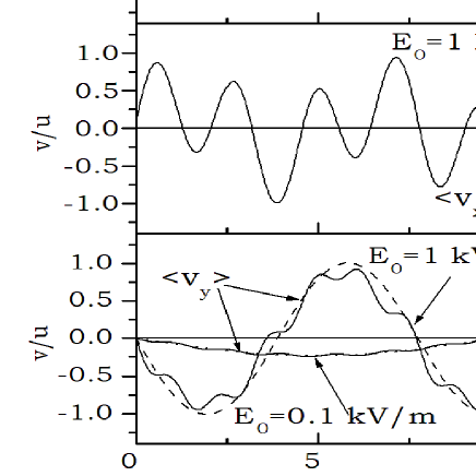
Figure 1: Average velocity of a delta-like packet in $x$ and $y$ directions versus time calculated numerically (solid lines) and within RWA (dashed lines). For $\langle v_{x}(t)\rangle$ the exact and RWA results are indistinguishable. Model parameters: $\omega_{D}=2\times 10^{12}$ s^-1 and $\omega_{Z}=2.31\times 10^{12}$ s^-1.

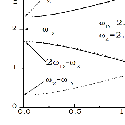
Figure 2: Frequencies of motion components for a delta-like wave packet versus electric field of EM wave. Upper line: ZB-like component of $\langle v_{x}\rangle$; middle line: satellite component of $\langle v_{x}\rangle$; lower line: $\langle v_{y}\rangle$ mode. Solid lines: exact results, dotted lines: approximations given by RWA.

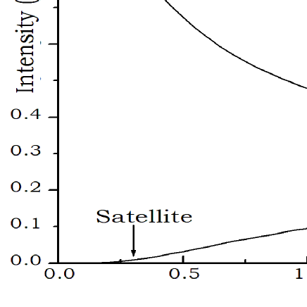
Figure 3: Intensities of ZB-like and satellite modes of $\langle v_{x}(t)\rangle$ calculated within RWA for a delta-like packet.

The rotating wave approximation (RWA) allows one to find approximate solutions of Eq. (3) when $\omega_{D}\simeq\omega_{Z}$ and the electric field $E_{0}$ is weak. We calculate average packet velocities in a few steps. First we note that, for a delta-like packet centered at ${\bm{k}}_{0}=(0,k_{0y})$, one may set $k_{x}=0$, which removes the $k_{x}$ dependence of the Hamiltonian in Eq. (3). Next we transform Eq. (3) with the unitary transformation: $\hat{S}_{x}=(1-i\sigma_{x})/\sqrt{2}$. This gives

$$i\frac{d\psi}{dt}=\left\{\omega_{e}\cos(\omega_{D}t)\sigma_{x}+uk_{y}\sigma_{z}\right\}\psi,$$ (15)

where $\psi=\hat{S}_{x}\Psi$. The initial condition is $\psi(0)=(1,-i)^{T}/\sqrt{2}$. We assume solutions of Eq. (15) to be of the form

$$\psi(t)=\left(\begin{array}[]{c}\psi_{1}(t)\\ \psi_{2}(t)\end{array}\right)=\left(\begin{array}[]{c}a_{1}(t)e^{-iuk_{y}t}\\ a_{2}(t)e^{+iuk_{y}t}\end{array}\right),$$ (16)

where $a_{1}(t)$ and $a_{2}(t)$ are unknown functions. On substituting $\psi(t)$ into Eq. (15) and neglecting terms oscillating with the frequency $\omega_{Z}+\omega_{D}$ one obtains

$$\frac{da_{1}}{dt} \simeq -i\frac{\omega_{e}}{2}e^{+i\Delta t}a_{2},$$ (17)

$$\frac{da_{2}}{dt} \simeq -i\frac{\omega_{e}}{2}e^{-i\Delta t}a_{1},$$ (18)

where $\Delta=\omega_{Z}-\omega_{D}$ with $\omega_{Z}=2uk_{y}$ being the interband ZB frequency. After some algebra we find

$$\psi_{1}(t) = C_{+}e^{-i\omega_{D}t/2+i\omega_{R}t/2}+C_{-}e^{-i\omega_{D}t/2-i\omega_{R}t/2},\ \ \ \ \$$ (19)

$$\psi_{2}(t) = D_{+}e^{+i\omega_{D}t/2+i\omega_{R}t/2}+D_{-}e^{+i\omega_{D}t/2-i\omega_{R}t/2},\ \ \ \ \$$ (20)

where $C_{\pm}$ and $D_{\pm}$ are constants determined from the initial condition, and

$$\omega_{R}=\sqrt{\left(\omega_{Z}-\omega_{D}\right)^{2}+\left(\frac{eE_{0}u}{\hbar\omega_{D}}\right)^{2}}.$$ (21)

The obtained frequency  (21) corresponds to the generalized Rabi frequency appearing in the oscillating occupation of periodically driven two-level systems Rabi1937 ; BoydBook . Having $\psi(t)=\hat{S}_{x}\Psi(t)$ we calculate the average velocities, see Eqs. (9) and (10)

$$\langle v_{x}(t)\rangle = \frac{u}{2}\left(1+\frac{\Delta}{\omega_{R}}\right)\sin(\omega_{D}t+\omega_{R}t)$$ (22)

$$+ \frac{u}{2}\left(1-\frac{\Delta}{\omega_{R}}\right)\sin(\omega_{D}t-\omega_{R}t),$$

$$\langle v_{y}(t)\rangle = -u\frac{\omega_{e}}{\omega_{R}}\sin(\omega_{R}t).$$ (23)

Equation (22) describes electron motion oscillating with two frequencies:

$$\omega_{\pm}=\omega_{D}\pm\omega_{R},$$ (24)

Let us consider the case of small electric fields and $\omega_{D}<\omega_{Z}$. From Eq. (21) there is $\omega_{R}\simeq\omega_{Z}-\omega_{D}$, so that the frequency in the first line of Eq. (22) is $\omega_{D}+\omega_{R}\simeq\omega_{Z}$, i.e. it corresponds to the Zitterbewegung frequency in the field-free case. The second frequency (satellite, SAT) equals then to $2\omega_{D}-\omega_{Z}$. Since $\Delta=\omega_{Z}-\omega_{D}>0$, the amplitude of the satellite approaches zero, while the amplitude of ZB part approaches unity. For $\omega_{D}>\omega_{Z}$ the roles of the first and second contributions to the velocity are reversed. The $y$ component of motion oscillates with the generalized Rabi frequency $\omega_{R}$ and its amplitude is proportional to the field intensity. In general, the $\langle v_{y}(t)\rangle$ component is not related to the ZB oscillations. However, the Rabi frequency includes the ZB frequency $\omega_{Z}$, so at low fields $E_{0}$ one can measure $\omega_{Z}$ from the relation $\omega_{R}\simeq|\omega_{Z}-\omega_{D}|$.

Results for $\langle v_{x}(t)\rangle$ calculated for two electric fields are plotted in Fig. 1a and Fig. 1b, while in Fig. 1c we show results for $\langle v_{y}(t)\rangle$. The solid lines show the results obtained numerically by solving Eq. (3) with the use of fifth-order Runge-Kutta method, while the dashed lines are obtained within RWA from Eq. (23). Here the parameters are within the range of validity of RWA and the average velocity $\langle v_{x}(t)\rangle$, as calculated numerically, is undistinguishable from the motion obtained with the use of Eq. (22). However, for larger fields there exist deviations from the RWA results for $\langle v_{y}(t)\rangle$, because for $\langle v_{y}(t)\rangle$ RWA predicts one frequency of oscillations, see Eq. (23), while the numerical calculations predict a small additional modulation.

The average packet velocity oscillates from $-u$ to $u$ and the motion does not disappear in time. The amplitude of $\langle v_{x}(t)\rangle$ does not depend on electric field. The frequencies of both ZB and SAT oscillations depend on the electric field and the frequency of the ZB mode differs from $\omega_{Z}=2uk_{0y}$. Patterns presented in Fig. 1a, 1b, and 1c are periodic in time. Using Fig. 1 we may define the Multi-mode Zitterbewegung as an appearance of additional oscillation modes in electron motion in the presence of an electromagnetic wave.

It is seen in Fig. 1c that the packet motion in the $y$ direction differs significantly from that in the $x$ direction. First, the amplitude of $\langle v_{y}(t)\rangle$ depends on the electric field: it vanishes for low fields and grows to $\pm u$ for large fields. Second, $\langle v_{y}(t)\rangle$ oscillates with one frequency for both low and high fields. Third, the amplitude of $\langle v_{y}(t)\rangle$ and the oscillation frequency strongly depends on the electric field. Finally, the oscillation frequency of $\langle v_{y}(t)\rangle$ is not related to $\omega_{Z}$.

Figure 2 shows frequencies of $\langle v_{x}(t)\rangle$ motion as functions of electric field $E_{0}$. The upper line describes the ZB-related frequency, while the middle line shows the satellite frequency. The lowest line presents the results for $\langle v_{y}(t)\rangle$. Numerical values are indicated by the dotted lines, the solid lines are obtained from the RWA formulas presented above. There is a very good agreement between the numerical results and those predicted by RWA.

Calculating the Fourier transform of $\langle v_{x}(t)\rangle$ we obtain the frequency spectrum $\langle v_{x}(\omega)\rangle$ of the motion. The intensities $I_{x}(\omega)$ of motion components are proportional to $|\langle v_{x}(\omega)\rangle|^{2}$. In Fig. 3 we show intensities of the ZB-like and satellite components determined by RWA. For $E_{0}=0$ the intensity of satellite vanishes and the packet oscillates with one frequency corresponding to the ZB frequency in the field-free case. For small fields, the ZB-like component dominates over the satellite component. By increasing the field one observes a gradual decrease of the ZB intensity and a slow growth of the satellite intensity. For still larger fields the intensities of both components are comparable.

III.2 High driving frequency (HDF)

To describe the electron motion for high driving frequency $\omega_{D}$ we consider again a delta-like wave packet centered around ${\bm{k}}_{0}=(0,k_{0y})$. By taking $k_{x}=0$ and transforming Eq. (3) with the use of unitary operator $\hat{S}_{y}=(1+i\sigma_{y})/\sqrt{2}$ one obtains

$$i\frac{d\phi}{dt}=\left\{\omega_{e}\cos(\omega_{D}t)\sigma_{z}+uk_{y}\sigma_{y}\right\}\phi,$$ (25)

where $\phi=\hat{S}_{y}\Psi$. The initial condition for $\phi$ is: $\phi(0)=(1,-1)^{T}/\sqrt{2}$. We assume solutions of Eq. (25) to be in the form

$$\phi(t)=\left(\begin{array}[]{c}b_{1}(t)e^{-i\kappa\sin(\omega_{D}t)}\\ b_{2}(t)e^{+i\kappa\sin(\omega_{D}t)}\end{array}\right),$$ (26)

where $\kappa=\omega_{e}/\omega_{D}$ and $b_{1}(t)$, $b_{2}(t)$ are unknown functions. On substituting $\phi(t)$ into Eq. (25) one has

$$i\frac{db_{1}(t)}{dt} = -iuk_{y}e^{+2i\kappa\sin(\omega_{D}t)}b_{2}(t),$$ (27)

$$i\frac{db_{2}(t)}{dt} = +iuk_{y}e^{-2i\kappa\sin(\omega_{D}t)}b_{1}(t).$$ (28)

The above equations are still exact. For $\kappa\ll 1/2$ we approximate $e^{\pm 2i\kappa\sin(\omega_{D}t)}\simeq 1$ and the above equations reduce to

$$i\frac{db_{1}(t)}{dt} \simeq -iuk_{y}b_{2}(t),$$ (29)

$$i\frac{db_{2}(t)}{dt} \simeq +iuk_{y}b_{1}(t),$$ (30)

which can be easily solved. Using Eq. (25) one obtains

$$\phi_{1}(t) = \frac{1-i}{2}e^{+i\omega_{k}t-i\Lambda}+\frac{1+i}{2}e^{-i\omega_{k}t-i\Lambda},$$ (31)

$$\phi_{2}(t) = -\frac{1+i}{2}e^{+i\omega_{k}t+i\Lambda}-\frac{1-i}{2}e^{-i\omega_{k}t+i\Lambda},$$ (32)

where $\Lambda(t)=\kappa\sin(\omega_{D}t)$. Using Eqs. (9) and (10) we find components of the average velocity

$$\langle v_{x}(t)\rangle = u\sin(\omega_{Z}t),$$ (33)

$$\langle v_{y}(t)\rangle = u\sin(2\Lambda)\cos(\omega_{Z}t)$$ (34)

$$\simeq u\frac{\omega_{e}}{\omega_{D}}[\sin(\omega_{D}t-\omega_{Z}t)+\sin(\omega_{D}t+\omega_{Z}t)].$$

For high driving frequency the average velocity $\langle v_{x}(t)\rangle$ oscillates with one frequency $\omega_{Z}$ as in field-free case. One can interpret this result by saying that the electron cannot follow such a high frequency, so the effect of the wave averages to zero. The second motion component oscillates with two frequencies $\omega=\omega_{D}\pm\omega_{Z}$. Validity of the above approximation requires a small value of the parameter

$$\kappa=\frac{\omega_{e}}{\omega_{D}}=\frac{eE_{0}u}{\hbar\omega_{D}^{2}}\ll\frac{1}{2}.$$ (35)

Therefore, for fixed $E_{0}$, the parameter $\kappa$ decreases quadratically with $\omega_{D}$.

III.3 Numerical results

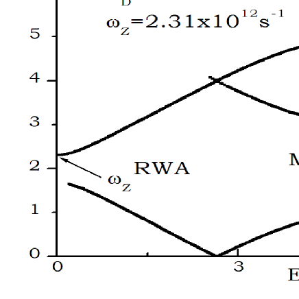
Figure 4: Main frequencies of MZB motion calculated for a delta-like wave packet vs. electric field of the wave in $\omega_{D}\simeq\omega_{Z}$ regime.

From Fig. 3 we see that for $E_{0}\geq$ 1 kV/m the amplitudes of both motion components are comparable. Thus a strong driving wave changes a single-frequency motion into a two-frequency motion. It is expected that still higher electric fields lead to appearance of even more components. To verify this expectation we calculate numerically the average packet velocity for large electric fields. Next we carry out the Fourier transform of $\langle v_{x}(t)\rangle$ and identify main frequencies in the motion.

For given $\bm{k}=(0,k_{0y})$, the numerical calculations of the wave function $\Psi(t)$ in Eq. (3) are performed using the fifth-order Runge-Kutta method. Having determined $\Psi(t)$ we calculate the average velocity with the use of Eq. (9) as a function of electric field $E_{0}$. The results are shown in Fig. 4. For each value of $E_{0}$ we plot components of $\langle v_{x}(t)\rangle$ for which the absolute value of its Fourier transform exceeds the threshold defined below. Assuming that the Fourier spectrum $\langle v_{x}(\omega)\rangle$ is normalized as: $\int|\langle v_{x}(\omega)\rangle|d\omega=1$ we take the threshold at the level: $|\langle v_{x}(\omega)\rangle|>0.05$. For low electric fields the packet motion has two frequencies and it is well described by RWA. The field intensity corresponding to apparent zero frequency (just below $E_{0}=$ 3kV/m) determines the upper range of validity of RWA. For still larger fields a nonlinear wave mixing appears and the number of motion frequencies increases to three, four, etc. Note that the additional frequencies appear gradually, i.e. their amplitudes grow from zero. They are plotted in Fig. 4 when their intensities exceed the threshold mentioned above. The same can be said about the bifurcation point close to $E_{0}\simeq$ 3 kV/m: the lower branch appears gradually and the upper branch gradually disappears.

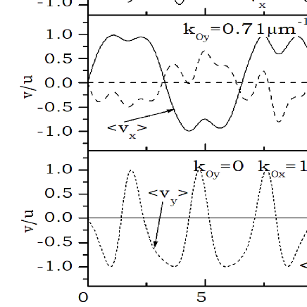
Figure 5: Average velocities $\langle v_{x}(t)\rangle$ and $\langle v_{y}(t)\rangle$ of a delta-like packet with different values of $k_{0y}$ and $k_{0x}$. Electric field is $E_{0}=1$ kV/m and $\omega_{D}=2\times 10^{12}$ s^-1. For $k_{0y}=0$ there is no motion in $x$ direction.

Until now we concentrated on the delta-like wave packet with a nonzero wave vector in the $y$ direction. Now we analyze the Multi-mode ZB for the delta-like packet with an arbitrary direction of the initial wave vector, i.e. ${\bm{k}}_{0}=(k_{0x},k_{0y})$. In the calculations we keep the same length of the wave vector, but change its direction. Equation (3) is solved numerically for three values of ${\bm{k}}_{0}$, the results are plotted in Fig. 5. Comparing maxima or minima of $\langle v_{x}(t)\rangle$ in Fig. 5a and Fig. 5b we note that the main oscillation frequencies remain almost unchanged. Finally, when $k_{0y}=0$, there is no electron motion in the $x$ direction but there is still motion in the $y$ direction, see Fig. 5c. This result is in agreement our earlier predictions, see Eqs. (11) and (12).

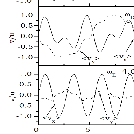
Figure 6: Average velocities $\langle v_{x}(t)\rangle$ and $\langle v_{y}(t)\rangle$ calculated for a delta-like packet for three values of $\omega_{D}$. Electric field is $E_{0}=1$ kV/m.

In Fig. 6 we show numerical results for another arrangement, when one keeps the electric field constant but changes the driving frequency. When $\omega_{D}$ is much smaller than $\omega_{Z}$, see Fig. 6a, the motion consists of many modes. When both frequencies are equal, see Fig. 6b, the motion has two well defined frequencies. For $\omega_{D}$ larger than $\omega_{Z}$, see Fig. 6c, the electron oscillates with one frequency equal to $\omega_{Z}$, the same as in the field-free case. This situation corresponds to the HDF case analyzed in the previous subsection and the numerical calculations confirm the validity of the HDF approximation.

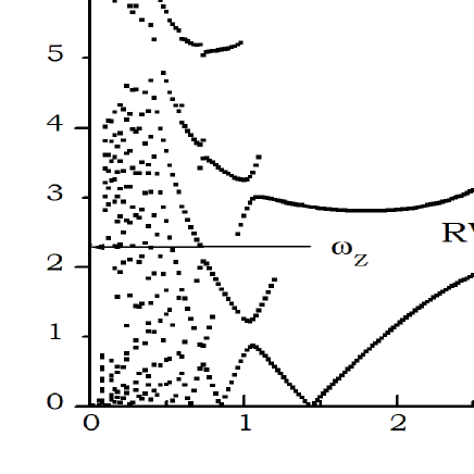
Figure 7: Main frequencies of MZB motion calculated for a delta-like wave packet vs. driving frequency $\omega_{D}$. Three regimes are observed: $\omega_{D}\gg\omega_{Z}$ (one mode), $\omega_{D}\propto\omega_{Z}$ (two modes) and $\omega_{D}\ll\omega_{Z}$ (many modes).

In Fig. 7 we show the spectrum of Multi-mode ZB motion in the $x$ direction as a function of $\omega_{D}$ for fixed $E_{0}$. This figure summarizes the basic properties of the Multi-mode ZB. For large $\omega_{D}$ there is only one frequency, the same as in the field-free case. For $\omega_{D}\simeq\omega_{Z}$ there are two modes oscillating with modified ZB and satellite frequencies. This is the region of validity of RWA. The latter works correctly until one of the two frequencies goes to zero. Then the nonlinear wave mixing appears and the motion consists of modes oscillating with many frequencies. In this region it is possible to identify a limited range of $\omega_{D}$ giving two-band descriptions of the motion, as e.g. for the two lower branches near $\omega_{D}=1.1\times 10^{12}$ s^-1. The complicated structure of MZB in this region makes it difficult to identify the $\omega_{Z}$ frequency. The conclusion from Figs. 4 and 7 is that the most promising regions for experimental observation of ZB are: 1) small electric fields for  $\omega_{D}\simeq\omega_{Z}$ when RWA is valid, 2) large $\omega_{D}$ when one ZB frequency occurs.

IV Motion of Gaussian packet

The above analysis uses a narrow delta-like packet in ${\bm{k}}$ space including only one wave vector ${\bm{k}}={\bm{k}}_{0}$. The obtained results allow one to identify main features of MZB and to establish connection between numerical results and RWA or large $\omega_{D}$ approximations. However, weakness of the delta-like packets is that the latter are completely delocalized in space and their oscillations have a limited sense. For this reason one should consider packets of finite widths, which are well localized both in ${\bm{k}}$ and real spaces. A finite size of the packet allows one to calculate the average position and its average velocity interpreted as the group velocity. As shown previously Rusin2007b , a finite packet does not alter main features of ZB: oscillation frequency remains nearly constant for various packet widths and for wide packets (in real space) the amplitude of first oscillations is almost the same as that for delta-like packets. We expect the same similarities to occur for MZB. As pointed out by Lock Lock1979 , the wave packet oscillations disappear in time as a result of the Riemann-Lebesgue theorem. In consequence, the ZB motion has a transient character. The decay of motion is caused by the presence of wave packet and strongly depends on packet’s width $d$ Rusin2007b . The presence of electric wave introduces two additional parameters to the system: field intensity $E_{0}$ and driving frequency $\omega_{D}$ which alter, among other features, the decay time of the packet. As we show in next subsections, the decay times of MZB oscillations are longer than those for ZB alone.

IV.1 Average velocity

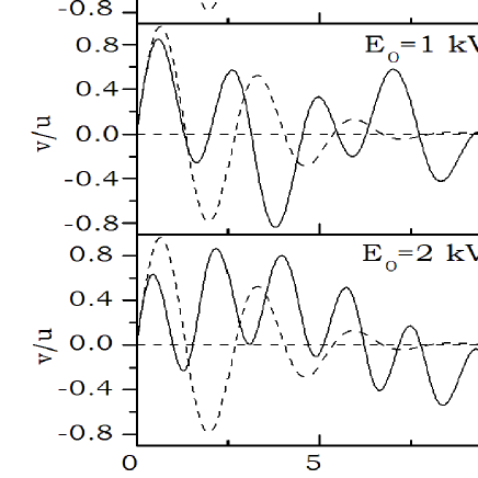
Figure 8: Average velocity $\langle v_{x}(t)\rangle$ of Gaussian packet for three electric fields. Driving frequency is $\omega_{D}=2\times 10^{12}$ s^-1 and $\omega_{Z}=2.31\times 10^{12}$ s^-1. Packet parameters: $d=4\mu$m; $k_{0x}=0$; $k_{0y}=1.2\mu$m^-1. Dashed lines: $\langle v_{x}(t)\rangle$ in absence of fields.

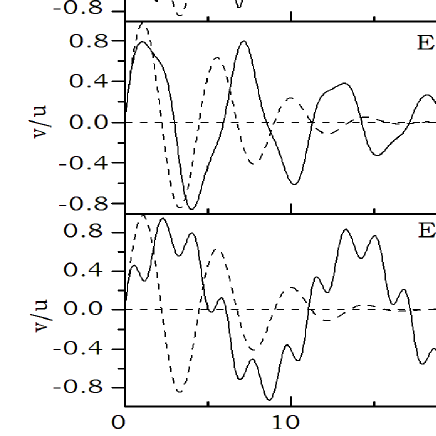
Figure 9: The same as in Fig. 8 but for a wider packet. Driving frequency is $\omega_{D}=2.0\times 10^{12}$ s^-1 and $\omega_{Z}=1.39\times 10^{12}$ s^-1. Packet parameters: $d=8\mu$m; $k_{0x}=0$, $k_{0y}=0.71\mu$m^-1. Dashed lines: $\langle v_{x}(t)\rangle$ in absence of fields.

Average packet velocities are calculated numerically using Eqs. (3), (9) and (10). First, we select the packet width $d$ and find a rectangle in the ${\bm{k}}$ space in which the Gaussian wave function in Eq. (5) does not vanish. In this rectangle we make a two-dimensional grid $N_{x}\times N_{y}$ of different ${\bm{k}}=(k_{x},k_{y})$ values. Next, for each point of the grid we solve numerically Eq. (3) using the fifth-order Runge-Kutta method. Finally, having $\Psi_{\bm{k}}(t)$ tabulated for all points in the grid and at all instants of time $t$, we calculate numerically, for each instant $t$, the double integrals over $d^{2}{\bm{k}}$ involved in average velocities in Eqs. (9) and (10). The integration is performed over all points of the grid in a standard way. Strong localization of the Gaussian packet in ${\bm{k}}$ space and proper normalization of $\Psi(t)$ for every $t$ ensures the convergence of the integrals. The results of all calculations presented in the next sections are obtained for $N_{x}=N_{y}=141$, i.e. for a given packet width Eq. (3) is solved 19881 times. We checked the accuracy of our calculations by increasing the grid up to $N_{x}=N_{y}=201$. Within the presented range of packet parameters the results are unchanged.

In Figs. 8 and 9 we show the MZB motion for two sets of packet parameters and four values of external driving field. The wave packet at $t=0$ is given in Eq. (5). Dashed lines indicate the field-free ZB motion, solid lines correspond to the motion in the presence of field (MZB). The parameters in Fig. 8 are in the region of validity of RWA. For a small field $E_{0}$, see Fig. 8a, the MZB oscillations follow pure ZB in terms of the oscillation frequency and amplitude, but they have much longer decay time. For larger fields, the MZB motion differs qualitatively and quantitatively from pure ZB oscillations. First, the MZB frequency is larger than for ZB. Second, MZB follows its delta-packet description (see Eq. (22)) and oscillates with two frequencies. Third, the decay time of MZB is much longer than the corresponding time of ZB, difference between the two is more than one order of magnitude. An intuitive explanation of the last difference is that the driving force, which persists in time, mixes with the transient ZB oscillation leading to a prolongation of MZB. A longer decay time of MZB oscillations should make a possible experimental detection of MZB easier.

The results shown in Fig. 9 are obtained for the driving frequency significantly larger than that of ZB. We observe a gradual transition from a two-frequency motion for low fields, see Fig. 9a, to a multi-frequency motion for large fields shown in Fig. 9c. The change in packet motion is similar to that shown in Fig. 4. Note the longer time oscillations seen in Fig. 9 as compared to the results in Fig. 8.

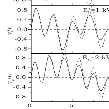
Figure 10: Average velocity $\langle v_{x}(t)\rangle$ of Gaussian packet (solid lines) compared with corresponding velocity of delta-like packet (dashed lines) having the same initial momentum $\hbar k_{0y}$ for three field intensities. Driving frequency is $\omega_{D}=2\times 10^{12}$ s^-1. Packet parameters are the same as in Fig. 8. It is seen that the finite width of the packet does not change oscillation frequency.

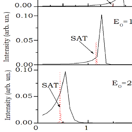
Figure 11: Frequency spectrum (not normalized) for Gaussian wave packet (solid lines) and delta-like packet (dotted lines) for three field intensities. Driving frequency is $\omega_{D}=2\times 10^{12}$ s^-1. Packet parameters are the same as in Fig. 8. For $E_{0}=0.5$ kV/m the intensity of satellite component is very small.

In Fig. 10 we compare the MZB oscillations for a Gaussian packet centered around ${\bm{k}}_{0}=(0,k_{0y})$ (solid lines) with those for a delta-like packet having the same wave vector ${\bm{k}}_{0}$ (dashed lines) for three values of electric field. The important feature of the decaying patterns is their nearly unchanged frequency, clearly visible in Fig. 10. The disappearance of the packet motion in time is characteristic of the wave packets Lock1979 . It is worth noting that the decay times of ZB-like oscillations shown in Figs. 8, 9 and 10 are in the scale of picoseconds, whereas those shown in Ref. Rusin2007b were in the scale of femtoseconds. The reason for this difference is that the widths of wave packets used in Ref. Rusin2007b were on the order of $d\simeq~{}40$ Å, while the widths used above are on the order $d\simeq~{}4$ $\mu$m. The general rule is that the wider the packet (i.e. narrower in the $k$-space), the longer the decay time of ZB oscillations.

In order to find precisely the frequency components of the motion we calculate the Fourier transform of the average packet velocity

$$\langle v_{x}(\omega)\rangle=\int_{-\infty}^{\infty}\langle v_{x}(t)\rangle e^{i\omega t}dt,$$ (36)

as well as the intensities of Fourier components $I_{x}(\omega)\propto|\langle v_{x}(\omega)\rangle|^{2}$. The results are shown in Fig. 11 by solid lines. They are compared to the power spectrum of a delta-like packet having the same wave vectors $k_{0y}=1.2\mu$m^-1 and $k_{0x}=0$ and marked with the delta-like dotted peaks. It is seen that the frequencies for the delta-like packets and the maxima for the Gaussian packets are close to each other for all electric fields.

IV.2 Sub-packets. Trajectories

It was shown previously that, in the field-free case, the fast decay of ZB oscillations results from a separation of sub-packets containing positive and negative energy states Rusin2007b . Here we carry a corresponding analysis for the time-dependent Hamiltonian in Eq. (2). For every instant of time this Hamiltonian can be expanded in the basis of its eigenstates $|1\rangle$ and $|2\rangle$

$$\hat{H}(t)=\lambda|1\rangle\langle 1|-\lambda|2\rangle\langle 2|,$$ (37)

where $\lambda=+\sqrt{H_{21}H_{12}}$ and

$$|1\rangle=\frac{1}{\sqrt{2}}\left(\begin{array}[]{c}1\\ H_{21}/\lambda\end{array}\right),\hskip 10.00002pt|2\rangle=\frac{1}{\sqrt{2}}\left(\begin{array}[]{c}-H_{12}/\lambda\\ 1\end{array}\right).$$ (38)

In the above expressions we treat $\hat{\bm{p}}$ as a c-number: ${\bm{p}}=\hbar{\bm{k}}$. Since the elements $H_{21}$ and $H_{12}$ of the Hamiltonian in Eq. (2) depend on time, also $\lambda$, $|1\rangle$ and $|2\rangle$ are functions of time. For $E_{0}\rightarrow 0$ the eigenvalue $\lambda(t)$ reduces to the electron energy in graphene: $\epsilon_{k}=u\hbar|k|$. In the absence of fields the states $|1\rangle$ and $|2\rangle$ reduce to the conduction and valence bands of graphene, respectively. At any instant of time one can expand the wave packet $\Psi(t)$

$$\Psi(t)=a_{1}|1\rangle+a_{2}|2\rangle,$$ (39)

where $a_{1}=\langle 1|\Psi\rangle$ and $a_{2}=\langle 2|\Psi\rangle$. Then we can expand the average packet velocity using the states $|1\rangle$ and $|2\rangle$ and obtain from Eq. (9)

$$\langle v_{x}(t)\rangle = |a_{1}|^{2}\langle 1|u\sigma_{x}|1\rangle+|a_{2}|^{2}\langle 2|u\sigma_{x}|2\rangle$$ (40)

$$+ a_{1}^{*}a_{2}\langle 1|u\sigma_{x}|2\rangle+a_{2}^{*}a_{1}\langle 2|u\sigma_{x}|1\rangle$$

$$\equiv \langle v_{x}^{11}(t)\rangle+\langle v_{x}^{22}(t)\rangle+\langle v_{x}^{12}(t)\rangle+\langle v_{x}^{21}(t)\rangle.\ \$$

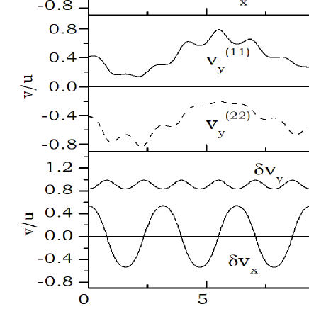
Figure 12: Average velocities of sub-packets corresponding to positive and negative energy states; a) motion of sub-packets in the $x$ direction; b) motion of sub-packets in the $y$ direction; c) relative velocity between the sub-packets. Electric field is $E_{0}=1$ kV/m and $\omega_{D}=2\times 10^{12}$ s^-1. Packet parameters are the same as in Fig. 8.

Terms in the first line of Eq. (40) describe the motion of centers of the two sub-packets, first with the positive and second with the negative eigenvalue $\lambda$. In the field-free case these terms lead to a rectilinear motion of sub-packets centers. In the presence of a driving wave these terms oscillate. Two terms in the second line of Eq. (40) describe an interference between the sub-packets. In the field-free case these terms are responsible for the ZB oscillations, and the same occurs in the presence of a driving field. These terms are nonzero when the sub-packets are close together, when they move away from each other the oscillations disappear. In Fig. 12a we plot the motion of sub-packet centers for $\langle v_{x}(t)\rangle$ calculated in Eq. (40). The velocities of sub-packets oscillate around $\langle v_{x}\rangle=0$ with similar frequencies but opposite phases. Thus, in the $x$ direction the sub-packets do not move away from each other.

In Fig. 12b we plot velocities of the two sub-packets in the $y$ direction using formulas analogous to that in Eq. (40). The motion is different from that in the $x$ direction. The velocities of sub-packets have different signs which means that they move in opposite directions. In Fig. 12c we show relative velocities of both sub-packets in $x$ and $y$ directions. The relative velocity in the $x$ direction oscillates around zero, which means that the sub-packets are close to each other, while the relative velocity in the $y$ direction is nearly constant with small superimposed oscillations. Thus the sub-packets move away each from other, cease to overlap and the MZB oscillations disappear similarly to the field-free case Rusin2007b .

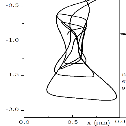
Figure 13: Trajectories of the packet and sub-packets consisting of states with positive and negative energies during first 35 ps of motion. a) trajectory of the packet; b) and c) trajectories of sub-packet having states positive (negative) energies. Electric field is $E_{0}=1$ kV/m and $\omega_{D}=2\times 10^{12}$ s^-1. Packet parameters are the same as in Fig. 8.

Packet trajectory can be calculated in two alternative ways. We can calculate the trajectory as an integral over the average velocity

$$\langle{\bm{r}}(t)\rangle=\int_{0}^{t}\langle{\bm{v}}(t^{\prime})\rangle dt^{\prime}.$$ (41)

Alternatively, one can calculate the trajectory directly

$$\langle{\bm{r}}(t)\rangle=\langle\Psi(t)|{\bm{r}}|\Psi(t)\rangle.$$ (42)

To find the trajectory in the $x$ direction we insert twice the unity operator and obtain

$$\langle x(t)\rangle = \sum_{{\bm{k}}{\bm{k}}^{\prime}}\langle\Psi|{\bm{k}}^{\prime}\rangle\langle{\bm{k}}^{\prime}|x|{\bm{k}}\rangle\langle{\bm{k}}|\Psi\rangle$$ (43)

$$= \frac{1}{4\pi^{2}}\int d^{2}{\bm{r}}\int d^{2}{\bm{k}}^{\prime}d^{2}{\bm{k}}\Psi_{\bm{k}^{\prime}}^{\dagger}\Psi_{\bm{k}}\left(e^{i{\bm{r}}{\bm{k}}}xe^{-i{\bm{r}}{\bm{k}^{\prime}}}\right),\ \ \$$

where $\Psi_{\bm{k}}$ is the solution of Eq. (3) for given ${\bm{k}}=(k_{x},k_{y})$ and the dagger means the Hermitian conjugate. If the function $\Psi_{\bm{k}}$ tends sufficiently fast to zero for large ${\bm{k}}$ (e.g. exponentially), one can change the order of integration in Eq. (43) and obtain

$$\langle x(t)\rangle = \frac{i}{4\pi^{2}}\int\Psi_{\bm{k}}^{\dagger}(t)\frac{\partial\Psi_{\bm{k}}(t)}{\partial k_{x}}d^{2}{\bm{k}},$$ (44)

$$\langle y(t)\rangle = \frac{i}{4\pi^{2}}\int\Psi_{\bm{k}}^{\dagger}(t)\frac{\partial\Psi_{\bm{k}}(t)}{\partial k_{y}}d^{2}{\bm{k}}.$$ (45)

Equations (44) and (45) give $\langle x(t)\rangle$ and $\langle y(t)\rangle$ at any instant of time, while Eq. (41) requires knowledge of $\langle{\bm{v}}(t^{\prime})\rangle$ for all $t^{\prime}\in(0,t)$. Choice of one of the two methods depends on details of the numerical procedure. For delta-like packets, Eq. (41) is more convenient because one does not deal with differentiation of the Dirac delta functions in Eqs. (44) and (45).

In Fig. 13a we show the calculated packet trajectory for the first 35 ps of motion and in Figs. 13b and 13c the trajectories of the two sub-packets. It is seen that the packet trajectory begins at ${\bm{r}}(0)={\bm{0}}$ and the packet moves in an irregular slowly converging orbit. In the field-free case the packet center is displaced only in the $x$ direction. The motion of sub-packets, as indicated in Figs. 13b and 13c, is different. The sub-packets move in opposite directions, so that their centers move away each from other. After 35 ps each of the sub-packets is displaced about 15 $\mu$m i.e. the distance between their centers exceeds the packet width $d$=4 $\mu$m. The results presented in Fig. 13 indicate that the mechanism responsible for the disappearance of MZB is similar to the field-free case Rusin2007b .

V Medium polarization

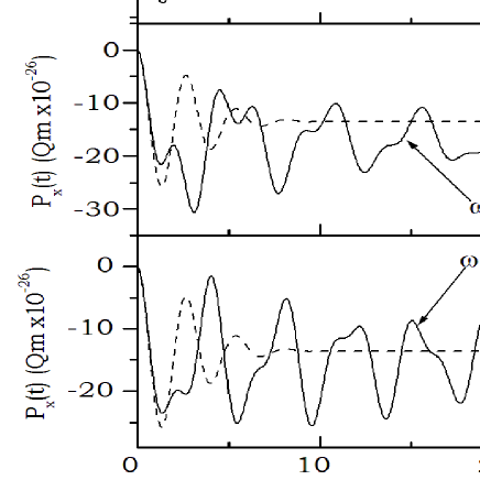
Figure 14: Polarization $P_{x}$ vs. time for four driving frequencies $\omega_{D}$. Dashed line: $P_{x}(t)$ in field-free case. Electric field is $E_{0}=1$ kV/m. Packet parameters are the same as in Fig. 8.

Now we turn to the medium polarization caused by the driving wave. The time-dependent polarization ${\bm{P}}(t)$ induced by the wave packet is a physical quantity measured frequently in the ultra-fast spectroscopy MukamelBook . Various experimental techniques allow one to determine packet motion from polarization oscillations in molecules ZewailNobel1999 , and quantum wells or superlattices Martini1996 ; Lyssenko1996 . The polarization is defined as

$$P_{x}(t)=-e\langle\Psi(t)|x|\Psi(t)\rangle,$$ (46)

and similarly for $P_{y}(t)$. Thus ${\bm{P}}(t)$ is proportional to the average packet position. The explicit forms of ${\bm{P}}(t)$ can be obtained from Eq. (41) or, equivalently, from Eqs. (44) and (45). In the time-dependent spectroscopy one expands polarization in the power series in field intensity ${\bm{E}}(t)$ BoydBook

$${\bm{P}}(t) = \epsilon_{0}\{\chi^{(1)}{\bm{E}}(t)+\chi^{(2)}{\bm{E}}^{2}(t)+\chi^{(3)}{\bm{E}}^{3}(t)+\ldots\}$$ (47)

$$= {\bm{P}}^{(1)}(t)+{\bm{P}}^{(2)}(t)+{\bm{P}}^{(3)}(t)+\ldots,$$

where $\chi^{(1)}$ is the linear susceptibility and $\chi^{(2)}$ and $\chi^{(3)}$ are non-linear susceptibilities of the second and third order, respectively. The above expansion assumes that the polarization depends on the instantaneous value of the electric field which implies that the system is lossless and dispersion-less BoydBook . In experiments, one can measure the linear polarization as well as the higher-order nonlinear polarizations using various techniques, e.g. photon echo or pump-and-probe measurements, see Ref. MukamelBook . In our approach we obtain in Eq. (47) an exact form of ${\bm{P}}(t)$ including all expansion orders. Connection between the third order polarizations observed in photon-echo experiments and the complete polarization, as given in Eq. (47), is discussed in Refs. Ebel1994 ; Seidner1995 .

In Fig. 14 we plot the time-dependent polarization $P_{x}(t)$ calculated for one electron prepared in the form of a Gaussian packet for five driving frequencies $\omega_{D}$. The derivatives of $\Psi(t)$ with respect to $k_{x}$ and $k_{y}$ are calculated numerically using the four-point differentiation rule. Dashed lines indicate polarization for $E_{0}=0$. In Fig. 14 we see different regimes of MZB oscillations: one frequency for large-driving frequency, two frequencies in the $\omega_{D}\simeq\omega_{Z}$ regime and many frequencies for low $\omega_{D}$. In Fig. 14a one can see that the polarization for large driving frequency nearly equals that for $\omega_{D}=0$. Thus for large $\omega_{D}$ the rapid oscillations of the driving wave average out to zero and they do not alter the electron motion. For $\omega_{D}$ close or smaller than $\omega_{Z}$ the decay time of polarization oscillations is about ten times longer than in the field-free case, which makes possible experimental observations easier. The decay time of $P_{x}(t)$ oscillations is longest for $\omega_{D}\simeq\omega_{Z}$, see Fig. 14c.

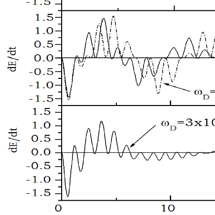
Figure 15: Instantaneous power $d{\cal E}/dt$ vs. time for three driving frequencies $\omega_{D}$. Electric field is $E_{0}=1$ kV/m. Packet parameters are the same as in Figure 8.

In the present work we concentrate on the average packet velocity. Now we analyze the observable quantity which allows one, at least in principle, to measure packet velocity in a direct way. Let us consider the time-dependent energy of the system: ${\cal E}=\langle\Psi|\hat{H}|\Psi\rangle$ Ebel1994 ; Seidner1995 . The change of ${\cal E}$ in time, i.e. the instantaneous power emitted or absorbed by the system is

$$I=\frac{d{\cal E}}{dt} = \langle\frac{d\Psi}{dt}|\hat{H}|\Psi\rangle+\langle\Psi|\hat{H}|\frac{d\Psi}{dt}\rangle+\langle\Psi|\frac{\partial\hat{H}}{\partial t}|\Psi\rangle$$ (48)

$$= \langle\Psi|\frac{\partial\hat{H}}{\partial t}|\Psi\rangle=-|e|E(t)\langle v_{x}(t)\rangle.$$

It is seen that the instantaneous power is proportional to the product of the electric field and the average velocity $\langle v_{x}(t)\rangle$. In Figure 15 we plot this power for four values of electric field. The results resemble those for $\langle P_{x}(t)\rangle$ but more frequencies appear. Note that, in experiments, it is more convenient to measure time-dependent polarization rather than the instantaneous power emitted or absorbed by the system. Thus the theoretical average velocity must be integrated over time in order to obtain the average position, see Eqs. (41) and (46).

VI Discussion

As we mention in the Introduction, our idea of considering the Multi-mode Zitterbewegung, i.e. the trembling motion of electrons in a periodic potential in an additional presence of a driving electromagnetic wave, was inspired by considerations of Super-Bloch-Oscillator Thommen2002 ; Kolovsky2009 ; Haller2010 . The two systems seem analogous, since both are characterized by an internal electron frequency related to the periodic lattice potential and in both the electrons are subjected in addition to the interaction with a driving wave. However, it turned out that our results do not much resemble those of the Super-Bloch-Oscillator. Rather, they are related to descriptions of systems consisting of two levels in the presence of a light wave i.e. to the problems in quantum optics. This affinity is expressed by similar mathematical elements, like the Heun function Heun2010 and the Mathieu equation mentioned above.

As to the quantum optics, it usually deals with levels, whereas we deal with bands, and it is mostly concerned with the population of levels, while we are interested in the electron motion. In quantum optics, one of the problems is that of gauge i.e. should the radiation be introduced by the electric scalar potential or by the vector potential. In our approach, we introduce the wave using the vector potential in the electric dipole approximation. This is a convenient choice and it leads to no ambiguities since we obtain exact numerical solutions which should be independent of the gauge.

We restrict our considerations to wave intensities $E_{0}<1\times 10^{6}$ V/m in order to avoid considerations of electron emission by the field. In this connection on should mention two issues. The first are the initial conditions for our treatment. We do not consider interband excitations of electrons in graphene by the incoming wave but assume from the beginning that the electron wave function has higher and lower components, see Eq. (4). This tacitly assumes that the Fermi level is located in the valence band of graphene, so that the electron wave packet can contain both components and their interference results in the Zitterbewegung.

The second issue is concerned with a possible emission of radiation. During the “classical” trembling motion in a solid the electron does not radiate because it is in the Bloch eigenenergy state. However, once the electron is additionally driven by an external wave, it is clearly not in the eigenenergy state and it can radiate. We do not consider here this radiation, we only consider a polarization of the graphene medium caused by the resulting motion. Also, our theory is a one-electron approach and we do not consider effects related to the fact that various electrons may oscillate with different phases.

We also neglect the effect of finite temperature on the electron oscillations. The driving frequency $\omega_{D}=2\times 10^{12}$ s^-1, which is often used in our paper, corresponds to the temperature $T_{D}=\hbar\omega_{D}/k_{B}\simeq 15.3$ K, so the experiments measuring the MZB should be performed in the liquid helium temperatures. A finite temperature would also lead, via the electron-phonon interaction, to a faster decay of MZB oscillations.

Another limiting factor of our approach is concerned with initial values of the wave vector characterizing the wave packet. This problem is present in almost all recent papers on Zitterbewegung, beginning with that of Schliemann et al. Schliemann05 . When one considers an electron localized in the form od a wave packet and takes its initial components $(1,0)^{T}$, see Eq. (4), it turns out that in order to have ZB in one direction one needs to have a non-vanishing initial momentum in the perpendicular direction. The question arises, how to create such momentum. If, which is tacitly assumed, the packet is created by a flash of laser light, the electron will have a very small initial momentum since that carried by light is small. An alternative way to create a sizable electron momentum would be to excite the electron by an acoustic phonon, but then the electron energy will be rather small. Still, in the simulation of the 1+1 Dirac equation by cold ions interacting with laser beams with the resulting ZB, as realized by Gerritsma et al. Gerritsma2010 , a non-vanishing momentum of the wave packet $(1,1)^{T}$ was created in the same direction. This suggests that the conditions considered in our approach could be created by an appropriate simulation. A system, in which a non-negligible initial momentum is present, are carbon nanotubes since there always exists a built-in quantized momentum in the direction perpendicular to the tube’s axis Rusin2007b ; Zawadzki2006 . It appears that, instead of taking a priori a packet in a given form, it would be more realistic to determine what packet forms are created in specific experiments and use these forms in subsequent calculations.

It is worth emphasizing that the two applied approximations, namely the rotating-wave and high driving frequency approximations give good results in two different regimes. The RWA applies to resonance conditions $\omega_{D}\simeq\omega_{Z}$, while HDF applies to $\omega_{D}\gg\omega_{Z}$ regime. As far as RWA is concerned the adopted procedure neglects frequencies away from the resonance, while in the HDF regime the condition of $\kappa=\omega_{e}/\omega_{D}\ll 1/2$ is well satisfied, see Eqs. (27), (27) and (35).

Finally, it should be mentioned that San Roman et al. Roman2003 described the Zitterbewegung of Dirac electrons driven by an intense laser field. According to a close analogy between relativistic Dirac electrons in a vacuum and electrons in narrow-semiconductors, see Ref. ZawadzkiHMF , this problem resembles ours since electrons in graphene, having a linear relation between the energy and momentum, represent the so called extreme relativistic case. However, the treatments in the two cases are different. The reason is that for the Dirac equation there exist Volkov solutions. They exist because the light velocity $c$ is the same as the maximum velocity of electrons. This is not the case for electrons in solids: the maximum velocity for electrons in graphene is around 300 times smaller than the light velocity. The description of Ref. Roman2003 for the Dirac electrons shows that the main effect of laser light is caused by its magnetic component, resulting in a collapse-and-revival pattern of ZB oscillations. This resembles the situation in graphene, as it has been shown that ZB in the presence of an external magnetic field exhibits the-collapse-and revival pattern, see Refs. Rusin2008 ; Romera2009 . On the other hand, since in the present paper we have neglected the magnetic component of the electromagnetic wave [see remarks after Eq. (2)] the effect of collapse-and-revival does not appear and we concentrate on the multi-mode behavior.

VII Summary

Electrons in monolayer graphene in the presence of an electromagnetic (or electric) wave are considered. It is shown that, in addition to the Zitterbewegung oscillations related to the periodic potential of graphene lattice, the electron interaction with the driving external wave gives rise to hybrid oscillations involving both the ZB frequency $\omega_{Z}$ and driving frequency $\omega_{D}$. Three distinct regimes of the motion are identified: one-frequency mode for $\omega_{D}\gg\omega_{Z}$, two-frequency mode for $\omega_{D}\simeq\omega_{Z}$, multi-frequency mode for $\omega_{D}\ll\omega_{Z}$, resulting from inherent nonlinearity of the system. Also, the presence of driving wave activates additional oscillation directions, not present in pure ZB motion. Dependence of the mode behavior on the intensity of driving wave is investigated. Electrons are described by either delta-like or Gaussian wave packets and it is shown that the essential oscillation characteristics (frequency and amplitude) depend only weakly on the packet width. It is indicated that the presence of a driving wave should facilitate observations of electron Zitterbewegung in semiconductors for two reasons: 1) It gives an additional external parameter for varying ZB-related frequency, 2) it prolongs the decay time of hybrid oscillations, as compared to that of pure ZB oscillations.

Appendix A Classical description

Here we briefly consider a classical description of a one-dimensional electron motion in the presence of a periodic potential and a driving electric wave. Let the periodic potential of the lattice be given by $W(x)=W_{0}\sin(2\pi x/a)$, where $a$ is the lattice period, and the interaction with the wave described by $eE_{0}x\cos(\omega_{D}t)$. Then the second Newton law of motion reads

$$m_{0}\frac{dv}{dt}=-W_{0}\left(\frac{2\pi}{a}\right)\cos\left(\frac{2\pi x}{a}\right)+eE_{0}\cos(\omega_{D}t),$$ (49)

where $m_{0}$ is the electron mass. We find approximate solutions of the above equation by iteration. In the initial step the velocity is taken to be constant and equal to $v_{0}$. This gives $x_{0}=v_{0}t$. By putting $x_{0}$ into Eq. (49) and integrating over time one obtains the first approximation to velocity

$$v_{1}(t)=-A_{1}\sin(\omega_{Z}t)+B_{1}\sin(\omega_{D}t),$$ (50)

where $\omega_{Z}=2\pi v_{0}/a$ is the frequency of Zitterbewegung [we put the initial value $v_{1}(0)=0$], and $A_{1}$, $B_{1}$ are constants. The first term in Eq. (50) describes oscillatory deviations of velocity from its average value $v_{0}$ due to ZB and the second accounts for the corresponding contribution of the wave. In this approximation there is no mixing of frequencies. Now one can again integrate the velocity of Eq. (50) over time to obtain $x_{1}(t)$ and put it back to the initial Eq. (49). This gives

$$m_{0}\frac{dv_{2}}{dt} = -W_{0}\frac{2\pi}{a}\cos\left[A_{1}\cos(\omega_{Z}t)+B_{1}\cos(\omega_{D}t)\right]$$ (51)

$$+eE_{0}\cos(\omega_{D}t).$$

It is seen that in the second approximation there is mixing of frequencies $\omega_{Z}$ and $\omega_{D}$. This mixing is a general feature of our nonlinear problem, it is seen in numerous expressions of the quantum treatment, see e.g. Eq. (22). In Eq. (34) one can also see a characteristic trigonometric function of a trigonometric function, appearing in the above classical expression (51).

Appendix B MZB vs. quantum optics

We find a correspondence between average velocities $\langle v_{x}(t)\rangle$ and $\langle v_{y}(t)\rangle$ in graphene and the probability of occupation of the upper level in the two-level model driven by a periodic force. This problem is frequently considered in quantum optics. The two-level model is usually described by the Schrodinger equation

$$i\frac{\partial\Phi}{\partial t}=\left\{\left[f_{0}+f_{1}\cos(\omega_{D}t)\right]\sigma_{x}+\frac{\nu}{2}\sigma_{z}\right\}\Phi.$$ (52)

It has been observed that solutions of the above equation can be expressed in terms of Heun functions Heun2010 . By introducing the unitary operator $\hat{S}_{x}=(1-i\sigma_{x})/\sqrt{2}$, acting with $\hat{S}_{x}$ on both sides of Eq. (3) and using $1=\hat{S}_{x}^{-1}\hat{S}_{x}$, one obtains

$$i\frac{\partial\Phi}{\partial t}=\left\{[uk_{x}+\omega_{e}\cos(\omega_{D}t)]\sigma_{x}+uk_{y}\sigma_{z}\right\}\Phi,$$ (53)

where $\Phi=\hat{S}_{x}\Psi$. Setting $f_{0}=uk_{x}$, $\nu=2uk_{y}$, and $f_{1}=\omega_{e}$ we transform the Hamiltonian of Eq. (3) into the Hamiltonian of the two-level model (52).

Let $\Phi(t)=(\Phi_{1}(t),\Phi_{2}(t))^{T}$. Then the probability of occupation of the upper level is $P^{up}=|\Phi_{1}(t)|^{2}$. On the other hand, using the projection operator $\hat{\cal P}^{up}$ of Eq. (56) the occupation probability of the upper state is $P^{up}=\langle\Phi|\hat{\cal P}^{up}|\Phi\rangle$. By using $\Phi=\hat{S}_{x}\Psi$ we find

$$P^{up}=\frac{1}{2}+\frac{1}{2}\langle\Psi|\sigma_{y}|\Psi\rangle,$$ (54)

which gives, see Eq. (9)

$$\langle v_{y}(t)\rangle=u\left(2P^{up}-1\right).$$ (55)

The above equation together with Eq. (53) connects the results for $P^{up}$ in the two-level model with the Zitterbewegung in graphene in the $y$ direction. Note that in quantum optics one calculates $P^{up}$ taking $\Phi(0)=(1,0)^{T}$, which gives $\Psi(0)=(1,i)^{T}$, while in ZB calculations one takes $\Psi(0)=(1,0)^{T}$.

Appendix C Relation to Rabi oscillations

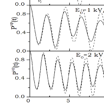
Figure 16: Occupation probability of the upper energy branch for Gaussian packets (solid lines) and delta-like packets (dashed lines) for three electric fields and $\omega_{D}=2\times 10^{12}$ s^-1. Dashed lines correspond to the Rabi oscillations in a two-level system. Packet parameters are the same as in Fig. 8.

Here we indicate relation between MZB and the Rabi oscillations, i.e. oscillations of the probability of occupation of upper (lower) energy states. For the upper energy level the projection operator is

$$\hat{\cal P}^{up}=\frac{1}{2}(1+\sigma_{z}),$$ (56)

and the occupation probability of the upper state (conduction band) is

$$\langle\hat{\cal P}^{up}\rangle=\langle\Psi(t)|\hat{\cal P}^{up}|\Psi(t)\rangle,$$ (57)

where $\Psi(t)$ is the solution of the Schrodinger equation (3). The probability $\langle\hat{\cal P}^{up}\rangle$ can be calculated in the way analogous to $\langle v_{x}(t)\rangle$. For the rotating wave approximation we obtain

$$\langle\hat{\cal P}^{up}\rangle = \frac{1}{2}+\frac{1}{2}\left(1+\frac{\Delta}{\omega_{R}}\right)\cos(\omega_{D}t+\omega_{R}t)$$ (58)

$$\ \ +\frac{1}{2}\left(1-\frac{\Delta}{\omega_{R}}\right)\cos(\omega_{D}t-\omega_{R}t),$$

while for the large $\omega_{D}$ approximation there is

$$\langle\hat{\cal P}^{up}\rangle = \frac{1}{2}+\frac{1}{2}\cos(2\Lambda)\cos(\omega_{Z}t)$$ (59)

$$\simeq \frac{1}{2}+\frac{1}{2}\cos(\omega_{Z}t).$$

Here $\Delta=\omega_{Z}-\omega_{D}$ and $\Lambda$ is given by Eq. (31). In Fig. 16 we show calculated Rabi oscillations for delta-like packets (dashed lines) and Gaussian packets (solid lines) for three values of external electric field. For the delta-like packets the oscillations are persistent while for the Gaussian packets they decay in time. The decay is caused by sub-packets moving in the opposite directions, as described above. The frequencies for delta-like packets are nearly equal to those of Gaussian packets. We do not pursue this subject here since the Rabi oscillations in graphene were treated in detail in Ref. Vasko2010 .

Appendix D Perturbation and Fer-Magnus expansions

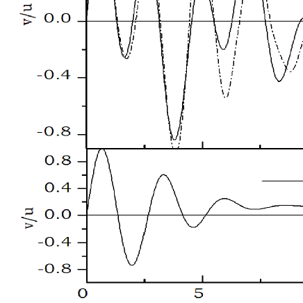
Figure 17: Average velocity $\langle v_{x}(t)\rangle$ of Gaussian packet calculated a) numerically (solid line), with the use of the Fer-Magnus expansion (dashed-dotted line) and b) using time-dependent perturbation. Electric field is $E_{0}=1$ kV/m and $\omega_{D}=2\times 10^{12}$ s^-1. Packet parameters are the same as in Fig. 8.

We compare our numerical time-dependent results with those obtained in the standard time-dependent perturbation and in the Fer-Magnus expansions. For small fields a natural way of finding approximate solutions of Eq. (3) is to treat the time-dependent term as a perturbation. Let $\varphi_{1}$ and $\varphi_{2}$ be the eigenstates of $\hat{H}_{0}$ corresponding to positive and negative energy states, respectively, and $\Psi_{1}(t),\Psi_{2}(t)$ be unknown eigenstates of complete $\hat{H}$.

We first express $\Psi(t)$ as a linear combination of $\Psi_{1}$ and $\Psi_{2}$

$$\Psi(t)=a_{1}\Psi_{1}(t)+a_{2}\Psi_{2}(t),$$ (60)

where $a_{1}$ and $a_{2}$ are time-independent coefficients to be found. In the lowest order of time-dependent perturbation there is

$$\Psi_{1}(t)\simeq\varphi_{1}e^{-i\omega_{k}t}+\frac{1}{i\hbar}\sum_{j=1,2}c_{1j}\varphi_{j}e^{-is_{j}\omega_{k}t}+\ldots,$$ (61)

where $\omega_{k}=u\sqrt{k_{x}^{2}+k_{y}^{2}}$, $s_{1}=+1$, $s_{2}=-1$, and

$$c_{1j}=\langle\varphi_{1}|\omega_{e}\sigma_{x}|\varphi_{j}\rangle\int_{0}^{t}\cos(\omega_{D}t^{\prime})e^{i\omega_{k}(s_{1}-s_{j})t^{\prime}}dt^{\prime}.$$ (62)

The expansion for $\Psi_{2}(t)$ is analogous. The coefficients $a_{j}$ in Eq. (60) can be found from the initial condition $\Psi(0)=(1,0)^{T}f({\bm{k}})$ for $E_{0}=0$. The matrix elements and the integration in Eq. (62) can be calculated analytically. Having the approximate form of $\Psi(t)$ we can calculate the average velocity $\langle v_{x}(t)\rangle$ for the wave packet. The results are shown in Fig. 17b. In Fig. 17a we plot the corresponding exact results for $\langle v_{x}(t)\rangle$ computed numerically.

Comparing the approximate results with the exact ones it can be seen that, in this problem, the first order time-dependent perturbation presents a poor approximation. First, for long times the perturbation gives a constant, nonzero velocity, while the exact results give vanishing velocity. Second, the decay time of MZB calculated by the perturbation is too short. Still, the perturbation expansion gives proper oscillation frequency and correct behavior of $\langle v_{x}(t)\rangle$ for short times.

Another possibility of obtaining approximate results is the Magnus expansion for the propagator of the Schrodinger equation with time-dependent Hamiltonians Magnus1954 . Having exact or approximate propagator $\hat{U}(t)$ one can calculate $\Psi(t)=\hat{U}(t)\Psi(0)$ and then the average velocity, see Eqs. (9) and (10). In our approach we examine the Fer-Magnus (FM) expansion, which is more suitable for problems periodic in time Fer1958 . The advantage of Magnus or FM expansions is that the propagator in Eq. (63) remains unitary in every order of perturbation, which ensures the proper norm of the wave function.

Following the suggestion of Blanes et al. Blanes2009 we transform Eq. (3) to the interaction picture $i\hbar d\Psi^{i}/dt=V^{i}(t)\Psi^{i}$, where $\Psi^{i}=e^{+i\hat{H}_{0}t/\hbar}\Psi$ and $V^{i}(t)=e^{i\hat{H}_{0}t/\hbar}V(t)e^{-i\hat{H}_{0}t/\hbar}$. In the Fer-Magnus expansion the propagator is assumed in the form

$$\hat{U}=\exp\left(-i\sum_{n=1}^{\infty}\hat{\Lambda}_{n}(t)\right)\exp\left(-it\sum_{n=1}^{\infty}\hat{F}_{n}\right),$$ (63)

where $\hat{\Lambda}_{n}(t)$ and $\hat{F}_{n}$ are given by recursive formulas Blanes2009 . At present there exist no closed formulas for $\hat{F}_{n}$ and $\hat{\Lambda_{n}}(t)$ with arbitrary $n$. For $n=1$ there is

$$\hat{F}_{1} = \frac{1}{T}\int_{0}^{T}V^{int}(t^{\prime})dt^{\prime},$$ (64)

$$\hat{\Lambda_{1}}(t) = \int V^{int}(t^{\prime})dt^{\prime}-t\hat{F_{1}}.$$ (65)

Expressions for $n=2,3$ are given in Ref. Mananga2011 . Having an approximate propagator $\hat{U}(t)$ for $n=1$ we calculate average packet velocity and the results are plotted in Fig. 17a by dash-dotted line. The FM method correctly approximates frequencies and amplitudes of MZB motion both for short and long times. For short times the agreement is very good, for longer times a shift of phase appears. The decay time calculated with the use of FM agrees quite well with that obtained numerically and the vanishing velocity is in agreement with the exact results. We conclude that the FM expansion can be applied to calculations of the MZB motion.

References

- (1) E. Schrodinger, Sitzungsber. Preuss. Akad. Wiss. Phys. Math. Kl. 24, 418 (1930). Schrodinger’s derivation is reproduced in A. O. Barut and A. J. Bracken, Phys. Rev. D 23, 2454 (1981).
- (2) R. Gerritsma, G. Kirchmair, F. Zahringer, E. Solano, R. Blatt, and C. F. Roos, Nature 463, 68 (2010).
- (3) W. Zawadzki and T. M. Rusin, J. Phys. Cond. Matt. 23, 143201 (2011).
- (4) W. Zawadzki, Phys. Rev. B 72, 085217 (2005).
- (5) J. Schliemann, D. Loss, and R. M. Westervelt, Phys. Rev. Lett. 94, 206801 (2005).
- (6) W. Zawadzki and T. M. Rusin, Phys. Lett. A 374, 3533 (2010).
- (7) W. Zawadzki, Acta Phys. Pol. 123, 132 (2013).
- (8) M. I. Katsnelson, Europ. Phys. J. B 51 157, (2006).
- (9) J. Cserti and G. David, Phys. Rev. B 74 172305, (2006).
- (10) G. M. Maksimova, V. Ya. Demikhovskii, and E. V. Frolova, Phys. Rev. B 78, 235321 (2008).
- (11) G. David and J. Cserti, Phys. Rev. B 81 121417(R), (2010).
- (12) T. M. Rusin and W. Zawadzki, Phys. Rev. B 76, 195439 (2007).
- (13) P. R. Wallace, Phys. Rev. 71, 622 (1947).
- (14) J. C. Slonczewski and P. R. Weiss, Phys. Rev. 109, 272 (1958).
- (15) J. W. McClure, Phys. Rev. 104, 666 (1956).
- (16) K. S. Novoselov, A. K. Geim, S. V. Morozov, D. Jiang, M. I. Katsnelson, I. V. Grigorieva, S. V. Dubonos, and A. A. Firsov, Nature 438, 197 (2005).
- (17) Q. Thommen, J. C. Garreau and V. Zehnle, Phys. Rev. A 65, 053406 (2002).
- (18) A. Kolovsky and H.J. Korsch, arXiv:0912.2587 (2009).
- (19) E. Haller, R. Hart, M. J. Mark, J. G. Danzl, L. Reichsollner, and H. C. Nagerl, Phys. Rev. Lett. 104, 200403 (2010).
- (20) L. Allen, and J. H. Eberly, Optical Resonance and Two-level Atoms (Wiley, New York, 1975).
- (21) W. P. Schleich, Quantum Optics in Phase Space (Wiley, Berlin, 2001).
- (22) B. M. Garraway and K. A. Suominen, Rep. Prog. Phys. 58, 365 (1995).
- (23) I. I. Rabi, Phys. Rev. 51, 652 (1937).
- (24) R. W. Boyd, Nonlinear Optics (Academic Press, San Diego, 2003).
- (25) J. A. Lock, Am. J. Phys. 47, 797 (1979).
- (26) S. Mukamel, Principles of nonlinear molecular spectroscopy (Oxford University Press, New York, 1995).
- (27) A. Zewail, Nobel lecture, (1999); available on http://nobelprize.org/nobel_prizes/chemistry/ laureates/1999/zewail-lecture.pdf.
- (28) R. Martini, G. Klose, H. G. Roskos, H. Kurz, H. T. Grahn, and R. Hey, Phys. Rev. B 54, R14325 (1996).
- (29) V. G. Lyssenko, G. Valusis, F. Loser, T. Hasche, K. Leo, M. M. Dignam, and K. Kohler, Phys. Rev. Lett. 79, 301 (1997).
- (30) G. Ebel and R. Schinke, J. Chem. Phys. 101, 1865 (1994).
- (31) L. Seidner, G. Stock, and W. Domcke, J. Chem. Phys. 103, 3998 (1995).
- (32) Q. Xie and W. Hai, Phys. Rev. A 82, 032117 (2010).
- (33) W. Zawadzki, Phys. Rev. B 74, 205439 (2006).
- (34) J. San Roman, L. Roso, and L. Plaja, J. Phys. B: At. Mol. Opt. Phys. 36, 2253 (2003).
- (35) W. Zawadzki, in High Magnetic Fields in the Physics of Semiconductors II, edited by G. Landwehr and W. Ossau (World Scientific, Singapore, 1997), p. 755.
- (36) T. M. Rusin and W. Zawadzki, Phys. Rev. B 78, 125419 (2008).
- (37) E. Romera and F. de los Santos, Phys. Rev. B 80, 165416 (2009).
- (38) P. N. Romanets and F. T. Vasko, Phys. Rev. B 81, 241411R (2010).
- (39) W. Magnus, Comm. Pure Appl. Math. 7, 649 (1954).
- (40) F. Fer, Bull. Classe Sci. Acad. Roy. Bel. 44, 818 (1958).
- (41) S. Blanes, F. Casas, J. A. Oteo, and J. Ros, Phys. Rep. 470, 151 (2009).
- (42) E. S. Mananga and T. Charpentier, J. Chem. Phys. 135, 044109 (2011).