Monte Carlo simulation of classical spin models with chaotic billiards

Abstract

It has recently been shown that the computing abilities of Boltzmann machines, or Ising spin-glass models, can be implemented by chaotic billiard dynamics without any use of random numbers. In this paper, we further numerically investigate the capabilities of the chaotic billiard dynamics as a deterministic alternative to random Monte Carlo methods by applying it to classical spin models in statistical physics. First, we verify that the billiard dynamics can yield samples that converge to the true distribution of the Ising model on a small lattice, and we show that it appears to have the same convergence rate as random Monte Carlo sampling. Second, we apply the billiard dynamics to finite-size scaling analysis of the critical behavior of the Ising model and show that the phase transition point and the critical exponents are correctly obtained. Third, we extend the billiard dynamics to spins that take more than two states and show that it can be applied successfully to the Potts model. We also discuss the possibility of extensions to continuous-valued models such as the XY model.

I Introduction

Many important classical spin models such as the Ising model and the Potts model are described as probability distributions of spin configurations. To investigate the behavior of such models numerically, we normally design Monte Carlo methods, and obtain samples from the model using random numbers. However, there is no reason in principle to use randomness for obtaining samples; it does not matter whether the samples are generated randomly or deterministically, if the samples properly represent the probabilistic models in question.

Chaotic Boltzmann machines recently proposed in Ref. Suzuki2013b have chaotic billiard dynamics that yields samples from Ising spin-glass models without any use of random numbers. They have been numerically shown to have computing abilities comparable to conventional (stochastic) Boltzmann machines. In this paper, we further numerically investigate the capabilities of the chaotic billiard dynamics as a deterministic alternative to random Monte Carlo methods for classical spin models. Although there have been no studies that utilize billiard dynamics for deterministic simulations of spin models, the following three streams of studies can be considered as closely related to the present study.

Firstly, several deterministic cellular automaton models for the Ising model have been proposed. The Q2R automaton Vichniac1984 is the simplest automaton model of the Ising model, and it evolves conserving the energy exactly. Creutz Creutz1986 proposed another automaton model in which demons are introduced as additional degrees of freedom. Demons absorb and release energy at each site conserving the total energy. Despite the simple and deterministic update rules, these models reproduce the probabilistic behavior of the Ising model. However, these automata cannot be directly regarded as deterministic samplers from the Ising model; in the Q2R automaton, spin configurations only move on a microcanonical ensemble, and in the Creutz automaton, the system temperature is internally determined. Although chaotic Boltzmann machines are not automata, there is a similarity to the Creutz automaton in the sense that the additional degrees of freedom introduced allows the system to deterministically generate samples from canonical ensembles.

Secondly, spin models based on coupled map lattices (CMLs) Kaneko1989 have been proposed Sakaguchi1988 ; Miller1993 ; Marcq1997 ; Marcq1998 ; Sakaguchi1999 ; Egolf2000 ; Just2006 . CMLs are typically composed of discrete-time chaotic elements on a lattice interacting with each other. They are known to exhibit rich spatio-temporal nonlinear dynamics, and form an important class of dynamical systems with a large number of degrees of freedom. By associating symbols to partitions in the state space of each element, CMLs can be regarded as deterministic Ising-like spin models. In the sense that the probabilistic behavior of Ising spins is realized by chaotic dynamics, CML-based spin models can be related to chaotic Boltzmann machines. However, each element constituting chaotic Boltzmann machines has continuous-time and non-chaotic dynamics.

Thirdly, it should be noted that random numbers used in conventional Monte Carlo simulations on ordinary computers, i.e., pseudo-random numbers, are deterministically generated. Therefore, in a sense, we have already been using deterministic Monte Carlo methods. Of course, such pseudo-random numbers are designed so that they can be regarded as truly random in many aspects. Since Monte Carlo methods rely on truly random numbers, it is crucial to use good random numbers in principle. However, the generation of good random numbers is costly, and this is one important issue in large-scale Monte Carlo simulations. Moreover, it has been pointed out Murray2012 that low-quality pseudo-random numbers can actually be used in Monte Carlo methods and may even improve the performance. Thus, it is controversial as to the quality of randomness actually required. It is also noteworthy that recently a deterministic sampling algorithm, which is called herded Gibbs sampling Bornn2013 , was proposed on the basis of the herding algorithm Welling2009 ; Welling2010 . Although the algorithm is not practical for large-scale simulations, it is theoretically far more efficient than conventional Monte Carlo methods. Thus, it is intriguing to explore what is possible with deterministic Monte Carlo algorithms, and chaotic Boltzmann machines can be regarded as one of the approaches to the problem.

With these motivations in mind, in this paper, we numerically investigate the capabilities of the chaotic billiard dynamics as a deterministic alternative to random Monte Carlo methods by applying it to classical spin models in statistical physics. We confirm that the billiard dynamics can yield samples that converge to the true distribution of the Ising model, and we show that the phase transition point and the critical exponents of the Ising model are correctly obtained. Furthermore, we extend the billiard dynamics to spins that take more than two states, and we apply it to the Potts model and the XY model. We also point out that the billiard sampling dynamics is reversible and can be a good example for discussing the microscopic origins of irreversible macroscopic behavior on the Ising model.

It is to be noted that although the term “Monte Carlo” may imply that the algorithm is probabilistic, we intentionally keep using this term for deterministic algorithms also, thereby indicating that they can be used exactly in the place of conventional Monte Carlo methods.

II Billiard dynamics for the Ising model

In this section, we briefly introduce the implementation of probabilistic spin models by billiard dynamics. Although we limit the description to the Ising model, it can be extended to arbitrary Ising spin-glass models or Boltzmann machines Suzuki2013b .

Let us consider the Ising model composed of $N$ sites on a lattice. The Hamiltonian for a spin configuration $\bm{\sigma}=(\sigma_{1},\dots,\sigma_{N})\in\{-1,+1\}^{N}$ of the Ising model is given by

$$E(\bm{\sigma})=-\sum_{\langle i,j\rangle}\sigma_{i}\sigma_{j},$$ (1)

where the summation is taken for all the adjacent pairs in a lattice.

The probability distribution of the spin configurations of the Ising model is given by the Gibbs distribution

$$\mathrm{P}[\bm{\sigma}]=\frac{1}{Z}\exp\left(-\frac{1}{T}E(\bm{\sigma})\right),$$ (2)

where $T$ denotes the temperature and $Z$ denotes the partition function given by

$$Z=\sum_{\bm{\sigma}}\exp\left(-\frac{1}{T}E(\bm{\sigma})\right).$$ (3)

For large spin systems, it is difficult to evaluate the probability and directly obtain the samples. To obtain samples from the probability distribution (2), we normally use Monte Carlo methods. Here we consider the heat-bath algorithm, which is also known as Gibbs sampling in the field of machine learning. We choose a spin $i$ from $1,\dots,N$ randomly or sequentially. For each chosen spin, we update the state according to the probability

$$\mathrm{P}[\sigma_{i}=+1\mid\bm{\sigma}_{\setminus i}]=\frac{\exp(\sum\sigma_{j}/T)}{\exp(\sum\sigma_{j}/T)+\exp(-\sum\sigma_{j}/T)},$$ (4)

where $\bm{\sigma}_{\setminus i}$ denotes the configuration of the spins in the system except for the $i$th spin. This process defines a Markov chain having the Gibbs distribution (2) as the stationary distribution. Therefore, we can eventually obtain a sample sequence from the Gibbs distribution.

Here, we consider using billiard dynamics instead of the heat-bath algorithm for sampling from the Gibbs distribution (2). We introduce an internal state $x_{i}\in[-1,+1]$ for each node $i$. The internal state of the $i$th node evolves according to the following differential equation:

$$\frac{\mathrm{d}x_{i}}{\mathrm{d}t}=-\sigma_{i}\exp\left(-\frac{1}{T}\sigma_{i}\sum_{j}\sigma_{j}\right).$$ (5)

The state of the $i$th node $\sigma_{i}$ changes when $x_{i}$ reaches $+1$ or $-1$ as follows:

$$\begin{split}\sigma_{i}\longleftarrow+1\quad\text{when}\quad x_{i}=+1,\\ \sigma_{i}\longleftarrow-1\quad\text{when}\quad x_{i}=-1.\end{split}$$ (6)

Note that $x_{i}$ decreases when $\sigma_{i}=+1$ and increases when $\sigma_{i}=-1$. Therefore, the internal state $x_{i}$ continues oscillating between $+1$ and $-1$. The continuous-time dynamics defined by Eqs. (5) and (6) is a hybrid dynamical system Aihara2010 on the state space $\{-1,+1\}^{N}\times[-1,+1]^{N}$, because it has both discrete and continuous state variables.

The differential equation (5) is designed to be consistent with Eq. (4) in the following sense. We assume here that the states of the neighboring nodes of the $i$th node are fixed. Then, $x_{i}$ oscillates between $+1$ and $-1$ periodically. According to Eq. (5), it takes $2\exp(\sum\sigma_{j}/T)$ unit time for $x_{i}$ to move from $+1$ to $-1$, and it takes $2\exp(-\sum\sigma_{j}/T)$ unit time for $x_{i}$ to move from $-1$ to $+1$. Hence, the period is $2(\exp(\sum\sigma_{j}/T)+\exp(-\sum\sigma_{j}/T))$ unit time, in which the state $\sigma_{i}$ takes on $+1$ for $2\exp(\sum\sigma_{j}/T)$ unit time. Therefore, the probability that we observe $\sigma_{i}=+1$ at a random instant is consistent with Eq. (4). Note that this consistency is derived under the assumption that the states of the neighboring nodes are fixed. Since the states in the system actually change, this is merely an explanation that justifies Eq. (5) only intuitively. It is expected but not assured that $\bm{\sigma}$ follows the Gibbs distribution (2).

In the explanation above, it is only essential that the relative time duration for which $\sigma_{i}$ takes on $+1$ in a period coincides with the probability $P[\sigma_{i}=+1\mid\bm{\sigma}_{\setminus i}]$ defined in Eq. (4). In other words, what is required for the consistency is that the speed $\left|\mathrm{d}x_{i}/\mathrm{d}t\right|$ is proportional to $P[\sigma_{i}\mid\bm{\sigma}_{\setminus i}]^{-1}$. In fact, there are two other natural implementations in place of Eq. (5). One possibility is to define the speed as $P[\sigma_{i}\mid\bm{\sigma}_{\setminus i}]^{-1}$ as follows:

$$\frac{\mathrm{d}x_{i}}{\mathrm{d}t}=-\sigma_{i}\left(1+\exp\left(-\frac{2}{T}\sigma_{i}\sum_{j}\sigma_{j}\right)\right).$$ (7)

Another possibility is to define the speed as $P[-\sigma_{i}\mid\bm{\sigma}_{\setminus i}]$ as follows:

$$\frac{\mathrm{d}x_{i}}{\mathrm{d}t}=\frac{-\sigma_{i}\exp(-\sigma_{i}\sum\sigma_{j}/T)}{\exp(\sum\sigma_{j}/T)+\exp(-\sum\sigma_{j}/T)}.$$ (8)

Considering the interactions with the neighboring nodes, these three definitions have different dynamics. As shown in the next section (Fig. 2(a)), all the definitions appear to work similarly, so that we mainly employ only Eq. (5) in this paper. We also note that implementations are not limited only to these three types. For instance, arbitrary constants different from site to site can be multiplied to the speeds.

There are two views on the dynamics of this system. If we focus on each node in the system, the internal state $x_{i}$ continues oscillating between $-1$ and $+1$, interacting with the neighboring nodes. In this sense, the system can be regarded as a type of coupled oscillator system. On the other hand, if we observe all the internal states simultaneously, the internal state $(x_{1},\dots,x_{N})$ travels in a straight line in the hypercube $[-1,+1]^{N}$ according to Eq. (5), and changes its direction when it collides with the boundary of the hypercube according to Eq. (6). In this sense, the dynamics of this system can be regarded as pseudo-billiard Blank2004 .

Unlike deterministic spin models implemented by CMLs, each node does not have chaotic dynamics. However, it has been shown Suzuki2013b ; Suzuki2013a that chaotic behavior naturally emerges from the interactions in the system, and it is considered to work as a heat-bath to realize probabilistic behavior of the spin configurations

Statistics of the Ising spin model can be obtained from the continuous-time billiard system in the following manner. Let $t_{0},t_{1},\dots,t_{k},\dots$ be the sequence of times at which state switchings occur according to Eq. (6). Then, the expectation value of a statistic $\Phi(\bm{\sigma})$ can be estimated from the samples until time $t_{K}$ as follows:

$$\langle\Phi\rangle=\frac{1}{t_{K}-t_{0}}\int_{t_{0}}^{t_{K}}\Phi(\bm{\sigma}(t))\mathrm{d}t=\frac{1}{t_{K}-t_{0}}\sum_{k=1}^{K}\tau_{k}\Phi(\bm{\sigma}_{k}),$$ (9)

where $\tau_{k}=t_{k}-t_{k-1}$ and $\bm{\sigma}_{k}$ denotes the state that the system is taking on in the time interval from $t_{k-1}$ to $t_{k}$. Thus, in a sense, we obtain a sample sequence $\bm{\sigma}_{1},\bm{\sigma}_{2},\dots$ weighted by time intervals $\tau_{1},\tau_{2},\dots$. The statistics are calculated in this manner in the present study. Another method to obtain a (unweighted) sample sequence is to observe $\bm{\sigma}=(\sigma_{1},\dots,\sigma_{N})$ uniformly, at every one unit time for example, or randomly. Note that sampling from a continuous-time billiard system is analogous to sampling with continuous-time (kinetic) Monte Carlo algorithms such as the Bortz–Kalos–Lebowitz (BKL) algorithm Bortz1975 and the Gillespie algorithm Gillespie1977 .

Although the billiard dynamics is described as a continuous-time system, numerical calculation can be carried out by iterating the Poincaré map $\bm{x}(t_{k})\mapsto\bm{x}(t_{k+1})$ induced on the boundary of the hypercube $[0,1]^{N}$ as explained in Refs. Suzuki2013b ; Suzuki2013a . Hence, when the system temperature is low and the spins seldom flip, the simulation performs efficiently, in a manner similar to continuous-time Monte Carlo algorithms. However, it is generally less efficient on ordinary computers compared with the ordinary heat-bath algorithm Suzuki2013b .

III Convergence

In this section, we numerically verify that the billiard dynamics yields samples that converge to the true distribution of the Ising model on a small lattice, for which probability distributions can be computed.

Figure 1: The absolute errors of the empirical distribution for the Ising model on a two-dimensional lattice of size $L=4$ with the periodic boundary condition at temperature $T=2.4$. The absolute error from the true distribution at time $t$ is calculated for the empirical distribution obtained from a trajectory until time $t$. The solid line indicates the average absolute error for 96 different trajectories, and the dashed lines indicate the minimum and maximum absolute errors among the trajectories. All the lines decrease at a gradient of nearly $-1/2$.

Figure 2: The absolute errors of the empirical distribution obtained by the billiard dynamics for the Ising model on a two-dimensional lattice with the periodic boundary condition. (a) The average absolute errors for different sampling algorithms. The lines indicated by “billiard1,” “billiard2,” “billiard3,” and “random” correspond to Eqs. (5), (7), (8), and random Monte Carlo sampling, respectively. (b) The average absolute errors for different lattice sizes $L=2,3,4$ at $T=2.4$. (c) The average absolute errors for different temperature values $T=2.0,2.4,2.8$ with $L=4$. All the lines shows the average absolute error for 96 different trajectories. Overall, the errors of billiard sampling dynamics decay very similarly to those of random sampling.

Figure 1 shows the absolute error between the empirical distribution observed from the billiard system and the true distribution of the Ising model on a two-dimensional lattice of size $L=4$. The absolute error is defined as

$$\sum_{\bm{\sigma}}\left|P[\bm{\sigma}]-\frac{r_{\bm{\sigma}}(t)}{t}\right|,$$ (10)

where $r_{\bm{\sigma}}(t)$ denotes the total time for which the system takes on the state $\bm{\sigma}$ until time $t$. The solid line in Fig. 1 indicates the absolute error averaged for 96 different initial values, and the dashed lines indicate the minimum and maximum errors. Note that the error is calculated for each orbit. Therefore, Fig. 1 shows that for all the 96 initial values randomly chosen from the uniform distribution on $\{-1,+1\}^{N}\times[-1,+1]^{N}$, the empirical distributions constantly converge to the true distribution. All the lines have gradients nearly equal to $-1/2$, thereby indicating that the convergence rate is almost $O(1/\sqrt{t})$.

Figure 2(a) shows the absolute errors for Eqs. (5), (7), (8), and random Monte Carlo sampling. As for random Monte Carlo sampling, $N$ Monte Carlo steps are regarded as one unit time. The errors decrease in a similar manner in each case. The constant biases between the algorithms are mainly due to the difference in the switching frequencies of the algorithms. This result numerically shows that all the three definitions for $\mathrm{d}x/\mathrm{d}t$, which are justified only intuitively in the previous section, work consistently with Eq. (4).

Figure 2(b) shows the absolute errors for different lattice sizes $L=2$, $3$, and $4$. The errors decrease at almost the same gradient. For calculation for $L=2$ and $3$, we perturbed the speeds of the units by multiplying constant values to Eq. (5). Specifically, Eq. (5) for $i=1,\dots,N$ is multiplied by $0.5+0.2i$ for $N=2\times 2$ and by $0.5+0.1i$ for $N=3\times 3$. Without this perturbation, the errors sometimes stop decreasing, which may be due to symmetries in these small systems composed of uniform units. For example, in the case of $L=2$, two units in diagonal positions receive exactly the same inputs from two other units in the other diagonal positions. Since it can be intuitively understood that the dynamics can be easily limited to a subspace if all the units are uniform, we perturbed the speeds and confirmed the convergence as expected.

Figure 2(c) shows the average absolute errors at different temperatures $T=2.0$, $2.4$, and $2.8$ for $L=4$. The errors decrease with almost the same gradient.

To summarize, all the results show convergence to the true distribution with the convergence rate almost in the order of $O(1/\sqrt{t})$. Namely, the convergence rate is almost the same as that of random Monte Carlo sampling, and slower than the order $O(1/t)$ of the herded Gibbs sampling Bornn2013 .

IV Finite-size scaling analysis

To examine the capabilities of the billiard dynamics for larger lattices, we apply it to finite-size scaling analysis (see, e.g., Ref. Newman1999 ) of the critical behavior of the Ising model. In the context of CMLs, it is known that the universality class depends on the updating rules Marcq1997 . Therefore, it is intriguing to determine as to which universality class the continuous-time billiard dynamics belongs to, although it should belong to the Ising universality class if the billiard dynamics truly yields samples from the Ising model precisely.

Figure 3: The Binder cumulant as a function of the temperature $T$ around $T_{\textrm{c}}$ for $L=32$, $40$, $48$, $56$, $64$, $72$, and $80$. (a) The points show the values of the Binder cumulant calculated numerically by the billiard dynamics. The statistics are calculated during $10^{7}$ unit time, after initial $10^{6}$ unit time is skipped, for 96 different initial values. The solid lines indicate least square fittings with cubic functions for each lattice size. (b) Magnification of the graphs in (a) around the critical temperature $T_{\textrm{c}}$. The intersections of the cubic fittings provides an estimate of $T_{\textrm{c}}=2.2690\pm 0.0002$, which is consistent with the theoretical critical temperature of $T_{\textrm{c}}=2/\log(1+\sqrt{2})=2.2691\cdots$ of the Ising model on a two-dimensional lattice indicated by the vertical line. Note that the graphs for larger lattices tend to give better estimates.

Figure 4: Dependencies on lattice size $L$ of (a) the gradient of the cubic fittings to the Binder cumulant $\partial U/\partial T$, (b) the mean absolute magnetization $\langle|m|\rangle$, and (c) the magnetic susceptibility $\chi$, all calculated at the theoretical critical temperature $T=T_{c}$. The crossings show the values obtained by numerical calculations. These log–log plots give the estimates (a) $1/\nu=0.993\pm 0.016$, (b) $\beta/\nu=0.1248\pm 0.0004$, and (c) $\gamma/\nu=1.751\pm 0.004$. These results are in agreement with the theoretical values of the critical exponents $\nu=1$, $\beta=1/8$, and $\gamma=7/4$ of the Ising model on a two-dimensional lattice. The lines show least square fits by linear functions with the theoretical gradient values.

We use the Ising model on a two-dimensional lattice of size $L=32,40,\dots,80$ with the periodic boundary condition. To find the phase transition point, we calculated the Binder cumulant Binder1981

$$U(L,T)=1-\frac{\langle m^{4}\rangle}{3\langle m^{2}\rangle^{2}},$$ (11)

where $m$ denotes the magnetization $m=\sum_{i}\sigma_{i}/N$. The graphs of the Binder cumulants for different lattice sizes $L$ are expected to intersect at the critical temperature $T_{c}$. Figure 3 shows the Binder cumulants calculated for various lattice sizes around the theoretical critical temperature and least square fittings with cubic functions to the calculated values. The intersections of the polynomial fits give an estimate of $2.2690\pm 0.0002$, which is consistent with the theoretical value of $T_{\textrm{c}}=2/\log(1+\sqrt{2})=2.2691\cdots$ of the Ising model on a two-dimensional lattice.

The exponent $\nu$ can be obtained from the derivative of the Binder cumulant with respect to the temperature at the critical temperature, because according to the finite-size scaling theory, the following relation holds:

$$\left.\frac{\partial U}{\partial T}\right|_{T=T_{c}}\propto L^{1/\nu}.$$ (12)

Figure 4(a) shows the derivatives of the polynomial fits at the theoretical critical temperature. The gradient of the log–log plot is estimated as $0.993\pm 0.016$, which is consistent with $\nu=1$ of the Ising model. The exponents $\beta$ and $\gamma$ can be obtained similarly from the absolute magnetization $\langle|m|\rangle$ and magnetic susceptibility $\chi=N(\langle m^{2}\rangle-\langle|m|\rangle^{2})$ at the critical temperature, using the following relation:

$$\langle|m|\rangle \propto L^{-\beta/\nu},$$ (13)

$$\chi \propto L^{\gamma/\nu}.$$ (14)

From the log–log plots shown in Fig. 4(b) and (c), the critical exponents $\beta/\nu$ and $\gamma/\nu$ are estimated as $0.1248\pm 0.0004$ and $1.751\pm 0.004$, respectively. These values are consistent with those of the Ising universality class: $\nu=1$, $\beta=1/8$, and $\gamma=7/4$.

V Potts model

In this section, we extend the billiard dynamics to spins that take more than two states, and we apply it to the Potts model. For simplicity, we describe the dynamics for the Potts model here; it is straightforward to extend the dynamics to more general spin systems.

The Hamiltonian of the $q$-state Potts model is given by

$$E(\bm{\sigma})=-\sum_{\langle i,j\rangle}\delta(\sigma_{i},\sigma_{j}),$$ (15)

where $\sigma_{i}\in\{0,1,\dots,q-1\}$ denotes the state of the $i$th site and $\delta(\cdot,\cdot)$ represents the Kronecker delta function.

We implement the Potts model on the basis of the billiard sampling dynamics for the Ising model as follows. We define an internal state $x_{i}\in\mathbb{R}/q\mathbb{Z}=[0,q)$ for each $i$th node, which evolves according to the following differential equation:

$$\frac{\mathrm{d}x_{i}}{\mathrm{d}t}=\exp\left(-\frac{1}{T}\sum_{j}\delta(\sigma_{i},\sigma_{j})\right).$$ (16)

Note that the speed $\mathrm{d}x_{i}/\mathrm{d}t$ is always positive and the two end points of $[0,q)$ are regarded as identical. Therefore, $x_{i}$ continues to increase in the interval $[0,q)$, and when it reaches $x_{i}=q$, it instantaneously jumps to $x_{i}=0$. The state $\sigma_{i}$ of the $i$th node is determined from $x_{i}$ as $\sigma_{i}=\lfloor x_{i}\rfloor$, where $\lfloor x_{i}\rfloor$ denotes the largest integer not greater than $x_{i}$.

Equation (16) is designed according to essentially the same idea as Eq. (5) of the billiard dynamics of the Ising model. Namely, the speed is determined so that it is proportional to $P[\sigma_{i}\mid\bm{\sigma}_{\setminus i}]^{-1}$. Therefore, when the probability is higher, the internal state moves more slowly, and the system remains in such a state for a longer duration.

This system can be regarded as a coupled oscillator system, because each internal state $x_{i}$ oscillates on a circle $\mathbb{R}/q\mathbb{Z}=[0,q)$ interacting with the neighboring nodes. When $q=2$, this system is essentially equivalent to the billiard dynamics for the Ising model. However, for $q>2$, the internal state $(x_{1},\dots,x_{N})$ travels on a $N$-dimensional torus $[0,q)^{N}$, and its dynamics cannot be reduced to a billiard system. Note that, as mentioned in Ref. Suzuki2013b , another implementation by pseudo-billiard dynamics for the Potts model is possible by using switched arrival systems Chase1993 .

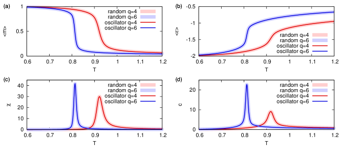
Figure 5: Statistics of the Potts model on a two-dimensional lattice of size $L=24$ with the periodic boundary condition for $q=4$ (red lines) and $q=6$ (blue lines) calculated by the heat-bath algorithm (thick lines) and the oscillator sampling dynamics (thin lines). (a) Average order parameter $\langle m\rangle$. (b) Average energy per site $\langle\epsilon\rangle$. (c) Magnetic susceptibility $\chi$. (d) Specific heat $c$. The statistics are calculated for $10^{5}$ unit time, after initial $10^{4}$ unit time is skipped, for 100 different initial values.

As a statistic that characterizes the behavior of the Potts model, we define the order parameter as follows:

$$m=\max_{s}\frac{qN_{s}-N}{N(q-1)},$$ (17)

where $N_{s}$ denotes the number of the sites taking on the state $s$. The order parameter $m$ takes $1$ when all the spins take one state ($\max_{s}N_{s}=N$) in the completely ordered phase, and it takes $0$ when the spins take all the states equally ($N_{s}=N/q$) in the completely disordered phase.

Figure 5 shows statistics of the Potts model on a two-dimensional lattice of size $L=24$ with the periodic boundary condition for $q=4$ and $q=6$ calculated by the heat-bath algorithm and the oscillator sampling dynamics. The Potts model on a two-dimensional lattice is known to undergo a second order phase transition if $q\leq 4$ and a first order phase transition if $q>4$. In Fig. 5, the average order parameter $\langle m\rangle$ and the average energy per site $\langle\epsilon\rangle=\langle E\rangle/N$ as well as their variances per site, the magnetic susceptibility $\chi=N(\langle m^{2}\rangle-\langle m\rangle^{2})$ and the specific heat $c=N(\langle\epsilon^{2}\rangle-\langle\epsilon\rangle^{2})$, are shown. In all the graphs, the lines for the two methods coincide with each other.

VI Discussion

VI.1 Extensions to continuous-valued spin models

The implementation for the Potts model naturally leads us to consider extensions to continuous-valued models such as the XY model. Here, we discuss the possibilities of such extensions.

The XY model is composed of spins that take continuous-valued states in $[0,2\pi)$. The Hamiltonian of the XY model is given by

$$E(\bm{\theta})=-\sum_{\langle i,j\rangle}\cos(\theta_{i},\theta_{j}),$$ (18)

where $\theta_{i}\in[0,2\pi)$ denotes the state of the $i$th spin. The XY model can be regarded as the limit $q\to\infty$ of the Potts model with the interaction term replaced by the cosine function.

One way to design sampling dynamics for the XY model on the basis of the oscillator dynamics for the Potts model is as follows. We define an internal state $x_{i}\in\mathbb{R}/\mathbb{Z}=[0,1)$ for each $i$th node. It evolves according to the following differential equation:

$$\frac{\mathrm{d}x_{i}}{\mathrm{d}t}=\exp\left(-\frac{1}{T}\sum_{j}\cos(\theta_{i},\theta_{j})\right).$$ (19)

Since $\mathrm{d}x_{i}/\mathrm{d}t$ is always positive, the internal state $x_{i}$ always increases from $0$ to $1$. When it reaches $x_{i}=1$, it instantaneously jumps to $x_{i}=0$ and the state $\theta_{i}$ is updated as follows:

$$\theta_{i}\longleftarrow\theta_{i}+2\pi\phi\quad\text{and}\quad x_{i}\longleftarrow 0\qquad\text{when}\quad x_{i}=1,$$ (20)

where $\phi$ is an arbitrary irrational number. We use the golden mean $\phi=(\sqrt{5}-1)/2$ in the numerical simulations.

Figure 6: The sampling dynamics for the XY model on a two-dimensional lattice of $L=8$ at $T=1.2$ (top row) and $T=0.6$ (bottom row). The absolute errors of empirical energy distributions from the distribution obtained by the Metropolis algorithm for $t=10^{8}$ are shown. The empirical energy distributions are constructed from samples until time $t$ generated by the (a) Metropolis algorithm, (b) irrational-rotation sampling dynamics, and (c) coupled-oscillator sampling dynamics. The solid lines indicate the average absolute error for 96 different sample sequences, and the dashed lines indicate the minimum and maximum absolute errors among the sequences.

As another possibility, it is natural to consider the limit $q\to\infty$ in the implementation for the Potts model (with the interaction term replaced by $\cos$). Then, the internal state $x_{i}$ can be viewed as the continuous-valued spin state $\theta_{i}$ of the XY model. More specifically, the state $\theta_{i}$ evolves according to the following differential equation:

$$\frac{\mathrm{d}\theta_{i}}{\mathrm{d}t}=\exp\left(-\frac{1}{T}\sum_{j}\cos(\theta_{i},\theta_{j})\right).$$ (21)

This equation defines a coupled oscillator system, although the interaction is completely different from ordinary coupled oscillator systems such as the Kuramoto model. Since the state changes continuously, the numerical simulation of this system is very different from other systems we have considered. In the following simulations, we integrate the differential equation by the fourth-order Runge-Kutta method with a time step of $0.01$.

We evaluate these methods by examining energy distributions constructed from sample sequences for the XY model at $T=1.2$ and $0.6$, where energy values per site are discretized with a bin width of 0.01. Since we do not have the true distribution, we regard an empirical distribution constructed from samples until $t=10^{8}$ generated by the Metropolis algorithm as the “true” distribution, where $N$ Metropolis steps are regarded as 1 unit time. Figure 6(a), (b), and (c) shows the absolute errors from the true distribution of the empirical distributions obtained by the Metropolis algorithm, the irrational-rotation sampling dynamics, and the coupled-oscillator sampling dynamics, respectively. For all the algorithms, sample sequences are obtained by sampling uniformly at every 1 unit time. As regards the irrational-rotation sampling (Fig. 6(b)), the error decreases almost in the order of $O(\sqrt{t})$ even in the worst case. While the coupled-oscillator sampling dynamics works well for $T=1.2$, it does not work at all for $T=0.6$ (Fig. 6(c)). We have not succeeded in tracking down the cause of this result yet; it is possible that Eq. (21) intrinsically does not offer proper sampling dynamics even if the equation can be integrated without numerical errors. Although it is also possible that this may be only due to numerical errors, this result at least shows that naive numerical integration does not work well.

To summarize, we have examined two types of sampling dynamics designed for continuous-valued spin models. While the irrational-rotation sampling dynamics (Eq. (19)) updates the state $\theta_{i}$ discretely, the coupled-oscillator sampling dynamics (Eq. (21)) updates the state $\theta_{i}$ continuously. Although the irrational-rotation sampling seems promising, further studies, especially on the differences between these two methods, are necessary to understand the capabilities and the limitations of the proposed dynamics.

VI.2 Spin echoes in the Ising model

Thus far, we have mainly described the billiard and oscillator sampling dynamics as a sampling method for classical spin systems. However, we note that the dynamics itself is also interesting as an abstract model for physical systems with a large number of degrees of freedom that can be related to both the CMLs and the coupled oscillator systems.

Figure 7: Observation of a spin echo in the Ising model on a two-dimensional lattice with size $L=64$ at $T=2.6$. A time series of the magnetization $m$ sampled uniformly at every $0.1$ unit time is shown. At time $t=0$, all the spins are aligned. At time $t=50$, all the internal states are flipped. Subsequently, at time $t=100$, the spins become aligned again.

One important aspect of the billiard sampling dynamics is its reversibility, while its macroscopic behavior as spin models is irreversible. The microscopic origins of irreversible macroscopic behavior have been an important topic in statistical physics since more than a century ago (see, e.g., Ref. Lebowitz1999 ). This topic has been discussed using models such as the Lorentz gas model (or Sinai’s billiard) Bunimovich1981 , multibaker maps Gaspard1992 ; Tasaki1995 , the Q2R automaton Stauffer2000 , and Nosé-Hoover thermostats Nose1984 ; Hoover1985 ; Hoover2012 . The billiard sampling dynamics also exhibits both reversible microscopic behavior and irreversible macroscopic behavior, and therefore, it can be a good example for discussing this topic, particularly if its chaotic dynamics is investigated in a more theoretical manner in the future. Note that the bakermap lattice Sakaguchi1999 for the Ising model can be a good example as well, because its dynamics is invertible and can be modified to be reversible.

As an example that demonstrates the reversibility, we show in Fig. 7 that spin echoes Hahn1950 can be observed in the Ising model with the billiard sampling dynamics. We use the Ising model in the paramagnetic (disordered) phase. At time $t=0$, all the spins are aligned to $+1$, so that the magnetization is initially equal to $1$. The initial internal state $\bm{x}$ is drawn from the uniform distribution on $[-1,+1]^{N}$. As the system equilibrates, the magnetization decreases to values around zero. At time $t=50$, we flip the signs of the internal states $\bm{x}$ instantaneously as $x_{i}\mapsto-x_{i}$, while the states $\bm{\sigma}$ are kept unchanged. After the flip, the simulation continues as if time is reversed. The magnetization remains in the equilibrium state for a while; however, it suddenly increases to $1$ at time $t=100$. Namely, all the spins are aligned again at the moment, contradictory to the second law of thermodynamics. This result is a natural consequence of the reversible dynamics, and theoretically, the memory of the initial state can be restored after an arbitrarily long time. However, it will practically become difficult to restore the initial state after a long equilibration time on a large lattice, due to the sensitive dependence on the initial conditions of the chaotic dynamics. This indicates that it will become almost impossible to find a microscopic state that evolves contrary to the second law of thermodynamics.

VII Summary

In this paper, we have numerically verified that the billiard dynamics can generate samples from the Ising model by examining the convergence and applying it to finite-size scaling analysis. We also have extended the billiard dynamics to multi-valued and continuous-valued spin models. In all the simulations (except for the oscillator dynamics for the XY model), the proposed dynamics works well as a deterministic alternative to random Monte Carlo sampling.

It is considered important to examine more spin models under various conditions on various network structures numerically. However, because there are infinitely many possible models to examine, we cannot clarify the capabilities and the limitations of this approach only by the means of numerical simulations. Therefore, we consider future studies on the theoretical foundations of the sampling dynamics to be also important on the basis of the promising results presented in this paper.

- (1) H. Suzuki, J. Imura, Y. Horio, and K. Aihara, Sci. Rep. 3, 1610 (2013).
- (2) G. Y. Vichniac, Physica 10D, 96 (1984).
- (3) M. Creutz, Ann. Phys. 167, 62 (1986).
- (4) K. Kaneko, Physica D 34, 1 (1989).
- (5) H. Sakaguchi, Prog. Theor. Phys. 80, 7 (1988).
- (6) J. Miller and D. A. Huse, Phys. Rev. E 48, 2528 (1993).
- (7) P. Marcq, H. Chaté, and P. Manneville, Phys. Rev. E 55, 2606 (1997).
- (8) P. Marcq and H. Chaté, Phys. Rev. E 57, 1591 (1998).
- (9) H. Sakaguchi, Phys. Rev. E 60, 7584 (1999).
- (10) D. A. Egolf, Science 287, 101 (2000).
- (11) W. Just, Phys. Rev. E 74, 046209 (2006).
- (12) I. Murray and L. T. Elliot, arXiv:1204.3187.
- (13) L. Bornn, Y. Chen, N. de Freitas, M. Eskelin, J. Fang, and M. Welling, arXiv:1301.4168 (submission for International Conference on Learning Representations, 2013).
- (14) M. Welling, in Proceedings of the 26th Annual International Conference on Machine Learning, Montreal, Canada, 2009 (ACM Press, New York, 2009), p. 1121.
- (15) M. Welling and Y. Chen, J. Phys.: Conf. Ser. 233, 012005 (2010).
- (16) K. Aihara and H. Suzuki, Phil. Trans. R. Soc. A 368, 4893 (2010).
- (17) M. Blank and L. Bunimovich, Dyn. Syst. 19, 359 (2004).
- (18) H. Suzuki, J. Imura, and K. Aihara, Sci. Rep. 3, 1127 (2013).
- (19) A. B. Bortz, M. H. Kalos, and J. L. Lebowitz, J. Comp. Phys. 17, 10 (1975).
- (20) D. T. Gillespie, J. Phys. Chem. 81, 2340 (1977).
- (21) M. E. J. Newman and G. T. Barkema, Monte Carlo Methods in Statistical Physics (Oxford University Press, New York, 1999).
- (22) K. Binder, Z. Phys. B 43, 119 (1981).
- (23) C. Chase, J. Serrano, and P. J. Ramadge, IEEE Trans. Automat. Control 38, 70 (1993).
- (24) J. L. Lebowitz, Rev. Mod. Phys. 71, S346 (1999); Physica A 263, 516 (1999).
- (25) L. A. Bunimovich and Ya. G. Sinai, Commun. Math. Phys. 78, 479 (1981).
- (26) P. Gaspard, J. Stat. Phys. 68, 673 (1992).
- (27) S. Tasaki and P. Gaspard, J. Stat. Phys. 81, 935 (1995).
- (28) D. Stauffer, Comp. Phys. Commun. 127, 113 (2000).
- (29) S. Nosé, J. Chem. Phys. 81, 511 (1984); Mol. Phys. 52, 255 (1984).
- (30) W. G. Hoover, Phys. Rev. A 31, 1695 (1985).
- (31) W. G. Hoover and C. G. Hoover, Time Reversibility, Computer Simulation, Algorithms, Chaos (World Scientific, 2012).
- (32) E. L. Hahn, Phys. Rev. 80, 580 (1950).