Frequency Domain Min-Max Optimization of Noise-Shaping Delta-Sigma Modulators

Abstract

This paper proposes a min-max design of noise-shaping delta-sigma ($\Delta\Sigma$) modulators. We first characterize the all stabilizing loop-filters for a linearized modulator model. By this characterization, we formulate the design problem of lowpass, bandpass, and multi-band modulators as minimization of the maximum magnitude of the noise transfer function (NTF) in fixed frequency band(s). We show that this optimization minimizes the worst-case reconstruction error, and hence improves the SNR (signal-to-noise ratio) of the modulator. The optimization is reduced to an optimization with a linear matrix inequality (LMI) via the generalized KYP (Kalman-Yakubovich-Popov) lemma. The obtained NTF is an FIR (finite-impulse-response) filter, which is favorable in view of implementation. We also derive a stability condition for the nonlinear model of $\Delta\Sigma$ modulators with general quantizers including uniform ones. This condition is described as an $H^{\infty}$ norm condition, which is reduced to an LMI via the KYP lemma. Design examples show advantages of our design.

I Introduction

Delta sigma ($\Delta\Sigma$, see Table I on the next page for the list of acronyms) modulators are widely used in oversampling AD (Analog-to-Digital) and DA (Digital-to-Analog) converters, by which we can achieve high performance with coarse quantizers [1, 2]. They have applications in digital signal processing systems, such as digital audio [3, 4] and digital communications [5, 6, 7]. More recently, the notion of $\Delta\Sigma$ modulators is extended to several research areas related to signal processing. In [8, 9, 10], the $\Delta\Sigma$ scheme is introduced for quantizing coefficients in finite but redundant frame expansion of signals, and is proved to outperform the standard PCM (pulse code modulation) scheme. Based on this study, $\Delta\Sigma$ scheme is also applied to compressed sensing [11, 12]. In [13, 14], dynamic quantizers as $\Delta\Sigma$ modulators are proposed for controlling linear time-invariant systems with discrete-valued control inputs. The $\Delta\Sigma$ scheme is also applied to obtain an approximate solution of large discrete quadratic programming problems [15]. For independent source separation [16] and manifold learning [17], machine learning is combined with $\Sigma\Delta$ modulation, called the $\Sigma\Delta$ learner.

In designing $\Delta\Sigma$ modulators, noise shaping is a fundamental issue [2].

Figure 1: $\Delta\Sigma$ modulator with loop-filter $H=[H_{1},H_{2}]$ and quantizer $Q$.

To describe the issue of noise shaping, let us consider a general $\Delta\Sigma$ modulator shown in Fig. 1. In this figure, $Q$ is a quantizer and $H=[H_{1},H_{2}]$ is a linear filter with 2 inputs and 1 output. The filter $H_{1}$ shapes the signal transfer function (STF) from the input $u$ to the output $y$ to have a unity magnitude in the frequency band of interest. On the other hand, the filter $H_{2}$ eliminates the in-band quantization noise by shaping the noise transfer function (NTF). Then, if the input signal $u$ is sufficiently oversampled, the frequency components in $u$ are concentrated in the band of interest, and hence one can effectively extract the original signal $u$ from the quantized signal $y$ by applying a lowpass filter to $y$ with a suitable cutoff frequency. In fact, it is theoretically shown that the reconstruction error decreases rapidly as the oversampling ratio increases [8, 18].

A usual solution to noise shaping is to insert accumulators (or integrators) in the feedback loop to attenuate the magnitude of the NTF in low frequency. To improve upon the performance, accumulators are cascaded in various ways such as the MASH (multi-stage noise-shaping) modulators [19, 20]. This methodology is analogous to a PID (Proportional-Integral-Derivative) control [21], in which the performance of the designed system depends on the experience of the designer. That is, the conventional design is of ad hoc nature.

To obtain a systematic design method, one can adopt a more general type of transfer functions than accumulators for $H(z)$ in Fig. 1. From this point of view, the NTF zero optimization [22, 2] was proposed to shape the NTF optimally in the frequency band of interest, say $[0,\Omega]$. This optimization is done by changing the zeros of the NTF so as to minimize the normalized noise power given by the integral of the squared magnitude of the NTF over $[0,\Omega]$. While this method gives a systematic way to design $\Delta\Sigma$ modulators, it can yield a peak in the magnitude of the NTF at a certain frequency, since such a peak cannot be captured by an integrated or averaged objective function. A recent paper [23] has investigated this problem and proposed to use semi-infinite programming for constraining the maximum value of a function over the frequency band. This method, however, does not necessarily optimize the overall performance but only minimizes the denominator of a loop-filter. That is, the method [23] does not necessarily reduce peaks in the NTF magnitude. Also, the computational cost for the optimization is very high due to its infinite dimensionality. Alternatively, the present authors has proposed to adopt $H^{\infty}$ optimization for attenuating the NTF magnitude itself with a frequency-domain weighting function [24]. This method gives a good performance if a suitable weighting function was chosen. For general notion of $H^{\infty}$ optimization in signal processing, see [25, 26]. The well-known Remez exchange method (aka Parks-McClellan method) [27] is related to the $H^{\infty}$ optimization. The method gives a near-optimal filter that minimizes the maximum error between a given desired filter and the filter to be designed. Strictly speaking, this is not $H^{\infty}$-optimal since the response is ignored on the transition frequency band.

In contrast to these methods, we propose a novel design based on min-max optimization, which can be reduced to finite dimensional convex optimization. That is, we directly minimize the maximum magnitude of the NTF over the frequency band of interest. In other words, we design $\Delta\Sigma$ modulators in order to uniformly attenuate the magnitude over the prespecified band. This uniform minimization improves the worst-case SNR (signal-to-noise ratio) to be defined in Section III-A, of the modulator in the band of interest. Conversely, a peak of the NTF magnitude as above can deteriorate the worst-case SNR and also the dynamic range of the modulator. We propose in this paper a more effective method that does not require a selection of a weighting function.

To this end, we first characterize all stabilizing loop-filters for a linearized modulator. Then, by using this parametrization, we formulate the design problem as an optimization via a linear matrix inequality (LMI) for lowpass and bandpass modulators using the generalized Kalman-Yakubovich-Popov (KYP) lemma [30, 25]. Furthermore, we can assign arbitrarily zeros of the NTF on the unit circle in the complex plane by adding a linear matrix equality (LME) constraint to the LMI. These techniques are mostly adopted from control theory. Recently, control theory is effectively applied to $\Delta\Sigma$ modulator design with finite horizon predictive control [31, 32], sliding mode control [33], and robust control [34, 35], to name a few. In particular, the idea of applying the generalized KYP lemma to $\Delta\Sigma$ modulator design is proposed in [36], in which they assume a one-bit quantizer for $Q$ and optimize the average power of the reconstruction error in low frequency for lowpass modulators. In contrast, our approach minimizes the worst reconstruction error, which can improve the overall SNR as mentioned above.

Stability analysis of $\Delta\Sigma$ modulators is another fundamental issue. For first-order [37] and second-order [38, 39] modulators, stability is well-studied in terms of invariant set. On the other hand, we derive a stability condition taking account of nonlinearity in $\Delta\Sigma$ modulators of arbitrary order with general quantizers including uniform ones. This condition is derived in terms of a state-space representation, and is described by the $\ell^{1}$ norm of a linear system. This can be transformed into an $H^{\infty}$-norm condition of the NTF as a sufficient condition. This $H^{\infty}$-norm constraint can be equivalently expressed as an LMI via the KYP lemma [40, 41, 25]. In summary, the proposed method can be described by LMI’s and LME’s, which can be solved effectively by numerical optimization softwares such as YALMIP [42] and SeDuMi [43] with MATLAB.

The organization of this paper is as follows: Section II gives characterization of all loop-filters that stabilize a linearized feedback modulator. Section III is the main section of this paper, in which we motivate the min-max design in view of SNR improvement, and then we formulate the design as a min-max optimization, which is reduced to LMI’s and LME’s. Section IV discusses stability of the $\Delta\Sigma$ modulator model without linearization. Section V introduces a cascade structure for high-order modulators. Section VI gives design examples to show advantages of our method. Section VII concludes our study.

Notation and Convention

Throughout this paper, we use the following notations. Abbreviations in this paper are summed up in Table I.

${\mathcal{S}}$, ${\mathcal{S}}^{\prime}$

$\mathcal{S}$ is the set of all stable, causal, and rational transfer functions with real coefficients, and ${\mathcal{S}}^{\prime}:=\{R\in{\mathcal{S}}:R\ \text{is strictly causal}\}$.

$\ell^{1}$

the Banach space of all real-valued absolutely summable sequences. For $\{v(k)\}_{k\geq 0}\in\ell^{1}$, the $\ell^{1}$ norm is defined by $\|v\|_{1}:=\sum_{k\geq 0}|v(k)|$.

$\ell^{\infty}$

the Banach space of all real-valued bounded sequences. For $\{v(k)\}_{k\geq 0}\in\ell^{\infty}$, the $\ell^{\infty}$ norm is defined by $\|v\|_{\infty}:=\sup_{k\geq 0}|v(k)|$.

$v\ast w$

convolution of two sequences $\{v(k)\}_{k\geq 0}$ and $\{w(k)\}_{k\geq 0}$, that is,

$$(v\ast w)(m):=\sum_{k\geq 0}v(m-k)w(k),\quad m=0,1,2,\dots.$$

For this computation, we set $v(m-k)=0$ if $m<k$.

TABLE I: Abbreviations

abbrev.	full name
$\Delta\Sigma$	Delta Sigma
NTF	Noise Transfer Function
STF	Signal Transfer Function
OSR	Over-Sampling Ratio
SNR	Signal-to-Noise Ratio
KYP	Kalman Yakubovich Popov
LMI	Linear Matrix Inequality
LME	Linear Matrix Equality

II Characterization of Loop-Filters

In this section, we characterize all $H(z)$’s that stabilize the linearized model shown in Fig. 2.

Figure 2: Linearized model for $\Delta\Sigma$ modulator with loop-filter $H=[H_{1},H_{2}]$.

This characterization is a basis for the proposed min-max design formulated in Section III. For a stability condition taking account of the nonlinear effect of the quantizer, see the discussion in Section IV.

We first define causality, stability, well-posedness and internal stability of linear systems.

Definition 1 (Causality and Stability)

A rational transfer function $P(z)$ is said to be (strictly) causal if the order of the numerator of $P(z)$ is (strictly) less than that of the denominator, and said to be stable if the poles of $P(z)$ are all in the open unit disk ${\mathbb{D}}=\{z\in{\mathbb{C}}:|z\rvert<1\}$.

Definition 2 (Well-posedness)

The feedback system in Fig. 2 is well-posed if there is at least one clock of delay in $H_{2}(z)$, that is, the transfer function $H_{2}(z)$ is strictly causal.

Definition 3 (Internal stability)

The feedback system Fig. 2 is internally stable if the four transfer functions from $[u,n]^{\top}$ to $[\psi,y]^{\top}$ are all stable.

We here characterize the filter $H(z)$ that makes the linearized feedback system well-posed and internally stable. All stabilizing filters are characterized as follows:

Proposition 1

The linearized feedback system in Fig. 2 is well-posed and internally stable if and only if

$$\begin{split}H_{1}(z)&=\frac{P(z)}{1+R(z)},\quad H_{2}(z)=\frac{R(z)}{1+R(z)},\\ P(z)&\in{\mathcal{S}},\quad R(z)\in{\mathcal{S}}^{\prime},\end{split}$$ (1)

where ${\mathcal{S}}$ denotes the set of all stable, causal, and rational transfer functions with real coefficients, and ${\mathcal{S}}^{\prime}:=\{R(z)\in{\mathcal{S}}:R(z)\ \text{is strictly causal}\}$.

Proof:

See Appendix -A. ∎

By using the parameters $P(z)\in{\mathcal{S}}$ and $R(z)\in{\mathcal{S}}^{\prime}$, we obtain the STF and NTF respectively as $T_{\text{\rm STF}}(z)=P(z)$ and $T_{\text{\rm NTF}}(z)=1+R(z)$. From this, it follows that the input/output equation of the system in Fig. 2 is given by

$$y=T_{\text{\rm STF}}~{}u+T_{\text{\rm NTF}}~{}n=Pu+(1+R)n.$$ (2)

By equation (2), the $\Delta\Sigma$ modulator can be realized by means of the design parameters $P(z)\in\mathcal{S}$ and $R(z)\in\mathcal{S}^{\prime}$ as shown in Fig. 3. This structure, called error-feedback structure [2] or noise-shaping coder [1], is often applied in the digital loops required in $\Delta\Sigma$ DA converters [2]. By this block diagram, we can interpret the filter $P(z)$ as a pre-filter to shape the frequency response of the input signal, and $R(z)$ as a feedback gain for the quantization noise $Q\psi-\psi$.

Figure 3: Error-feedback structure of $\Delta\Sigma$ modulator with design parameters $P(z)\in\mathcal{S}$ and $R(z)\in\mathcal{S}^{\prime}$.

III Optimal Loop-Filter Design via Linear Matrix Inequalities and Equalities

In this section, we propose a min-max design of the loop-filter $H(z)$ by using the parametrization in Proposition 1. First, we introduce the worst-case analysis of reconstruction errors in $\Delta\Sigma$ modulators to motivate the min-max design to be proposed. We then present design procedures for lowpass and bandpass modulators.

III-A Worst-case analysis of reconstruction errors

In oversampling lowpass $\Delta\Sigma$ converters with oversampling ratio $N_{\text{OSR}}$ (see Table I) [2], the authors attempt to attenuate the magnitude of the NTF in the frequency band ${\bm{I}}_{\text{B}}=[0,\Omega]\subset[0,\pi]$ where $\Omega=\pi/N_{\text{OSR}}$. In a bandpass converter, the band will be ${\bm{I}}_{\text{B}}=[\omega_{0}-\Omega,\omega_{0}+\Omega]$ where $\omega_{0}\in(0,\pi)$ is the center frequency. We here consider a general interval ${\bm{I}}_{\text{B}}\subset[0,\pi]$ in which the magnitude of the NTF is designed to be small. In a conventional design [22, 2], the attenuation level of the magnitude is measured by the average or the root mean square

$${\mathcal{N}}_{\text{average}}(T_{\text{\rm NTF}},{\bm{I}}_{\text{B}}):=\sqrt{\frac{1}{\lvert{\bm{I}}_{\text{B}}\rvert}\int_{{\bm{I}}_{\text{B}}}\lvert T_{\text{\rm NTF}}(\mathrm{e}^{\mathrm{j}\omega})\rvert^{2}\mathrm{d}\omega}.$$ (3)

On the other hand, we consider the worst-case measure

$${\mathcal{N}}_{\text{worst}}(T_{\text{\rm NTF}},{\bm{I}}_{\text{B}}):=\max_{\omega\in{\bm{I}}_{\text{B}}}\left\lvert T_{\text{\rm NTF}}(\mathrm{e}^{\mathrm{j}\omega})\right\rvert.$$ (4)

It is easy to see that ${\mathcal{N}}_{\text{worst}}$ gives an upper bound of ${\mathcal{N}}_{\text{average}}$, that is,

$${\mathcal{N}}_{\text{average}}(T_{\text{\rm NTF}},{\bm{I}}_{\text{B}})\leq{\mathcal{N}}_{\text{worst}}(T_{\text{\rm NTF}},{\bm{I}}_{\text{B}}).$$

Hence, minimization of ${\mathcal{N}}_{\text{worst}}(T_{\text{\rm NTF}},{\bm{I}}_{\text{B}})$ leads to small ${\mathcal{N}}_{\text{average}}(T_{\text{\rm NTF}},{\bm{I}}_{\text{B}})$, but not conversely. One can give an NTF with the same average ${\mathcal{N}}_{\text{average}}$ but much larger maximum magnitude ${\mathcal{N}}_{\text{worst}}$. That is, a small ${\mathcal{N}}_{\text{average}}$ does not necessarily yield a small ${\mathcal{N}}_{\text{worst}}$.

Another advantage of minimizing ${\mathcal{N}}_{\text{worst}}$ is the worst-case optimization of the reconstruction error $y-u$ (see Fig. 3). Define the worst-case reconstruction error ${\mathcal{E}}_{\text{worst}}$ by

$${\mathcal{E}}_{\text{worst}}:=\max_{\omega\in{\bm{I}}_{\text{B}}}\left\lvert\hat{y}(\mathrm{e}^{\mathrm{j}\omega})-\hat{u}(\mathrm{e}^{\mathrm{j}\omega})\right\rvert,$$

where $\hat{y}$ and $\hat{u}$ are, respectively, the discrete-time Fourier transforms of $y$ and $u$ in Fig. 3. Then this quantity can be described by the maximum magnitude ${\mathcal{N}}_{\text{worst}}(T_{\text{\rm NTF}},{\bm{I}}_{\text{B}})$ of $T_{\text{\rm NTF}}(z)$ over ${\bm{I}}_{\text{B}}$. In fact, we have the following proposition:

Proposition 2

Assume that the magnitude $\lvert\hat{n}(\mathrm{j}\omega)\rvert$ of the quantization noise $n=Q\psi-\psi$ is bounded on ${\bm{I}}_{\text{B}}$, that is, there exists $C_{0}>0$ such that $\max_{\omega\in{\bm{I}}_{\text{B}}}\lvert\hat{n}(\mathrm{e}^{\mathrm{j}\omega})\rvert=C_{0}$. Assume also that

$$\lvert T_{\text{\rm STF}}(\mathrm{e}^{\mathrm{j}\omega})\rvert=1,\quad\forall\omega\in{\bm{I}}_{\text{B}}.$$ (5)

Then the worst-case reconstruction error is given by

$${\mathcal{E}}_{\text{worst}}=C_{0}\cdot{\mathcal{N}}_{\text{worst}}(T_{\text{\rm NTF}},{\bm{I}}_{\text{B}}).$$ (6)

Proof:

By the relation

$$\begin{split}\hat{y}(\mathrm{e}^{\mathrm{j}\omega})&=T_{\text{\rm STF}}(\mathrm{e}^{\mathrm{j}\omega})\hat{u}(\mathrm{e}^{\mathrm{j}\omega})+T_{\text{\rm NTF}}(\mathrm{e}^{\mathrm{j}\omega})\hat{n}(\mathrm{e}^{\mathrm{j}\omega})\\ &=\hat{u}(\mathrm{e}^{\mathrm{j}\omega})+T_{\text{\rm NTF}}(\mathrm{e}^{\mathrm{j}\omega})\hat{n}(\mathrm{e}^{\mathrm{j}\omega}),\quad\forall\omega\in{\bm{I}}_{\text{B}},\end{split}$$

we have

$$\lvert\hat{y}(\mathrm{e}^{\mathrm{j}\omega})-\hat{u}(\mathrm{e}^{\mathrm{j}\omega})\rvert=\lvert T_{\text{\rm NTF}}(\mathrm{e}^{\mathrm{j}\omega})\hat{n}(\mathrm{e}^{\mathrm{j}\omega})\rvert,\quad\forall\omega\in{\bm{I}}_{\text{B}}.$$

By taking the maximum over the interval ${\bm{I}}_{\text{B}}$, we obtain (6). ∎

Note that the assumption (5) holds if we choose the pre-filter $P(z)$ that has a unity magnitude response over ${\bm{I}}_{\text{B}}$. In particular, if we take $P(z)=1$ then we have $T_{\text{\rm STF}}(z)=1$. By Proposition 2, optimization of ${\mathcal{N}}_{\text{worst}}$ improves the worst-case reconstruction error ${\mathcal{E}}_{\text{worst}}$. Minimizing ${\mathcal{N}}_{\text{worst}}$ also improves the peak-to-peak SNR (signal-to-noise ratio) of the modulator defined by

$$\mathrm{SNR}_{\text{pp}}(u):=\frac{\max_{\omega\in{\bm{I}}_{\text{B}}}\lvert\hat{u}(\mathrm{e}^{\mathrm{j}\omega})\rvert^{2}}{\max_{\omega\in{\bm{I}}_{\text{B}}}\lvert\hat{y}(\mathrm{e}^{\mathrm{j}\omega})-\hat{u}(\mathrm{e}^{\mathrm{j}\omega})\rvert^{2}}.$$ (7)

Figure 4: Peak-to-peak SNR for a narrow-band signal.

Let us consider the following set of input signals:

$${\mathcal{U}}:=\left\{u:\max_{\omega\in{\bm{I}}_{\text{B}}}\lvert\hat{u}(\mathrm{e}^{\mathrm{j}\omega})\rvert^{2}=1\right\}.$$

Suppose that the assumptions in Proposition 2 hold. Then, by Proposition 2, we have

$$\mathrm{SNR}_{\text{worst}}:=\min_{u\in{\mathcal{U}}}\mathrm{SNR}_{\text{pp}}(u)=\frac{1}{C_{0}{\mathcal{N}}_{\text{worst}}(T_{\text{\rm NTF}},{\bm{I}}_{\text{B}})}.$$

It follows that smaller ${\mathcal{N}}_{\text{worst}}$ leads to better worst-case SNR. Note that if condition (5) holds and if the input signal is sufficiently narrow-banded, $\mathrm{SNR}_{\text{pp}}$ can be estimated by the difference between the peak of $\hat{y}(\mathrm{j}\omega)$ and the peak of noise, or the maximum noise level in $\lvert\hat{y}(\mathrm{e}^{\mathrm{j}\omega})\rvert$, over the frequency range ${\bm{I}}_{\text{B}}$ (see Fig. 4).

Conversely, if ${\mathcal{E}}_{\text{worst}}$ is as large as $\max_{\omega\in{\bm{I}}_{\text{B}}}\lvert\hat{u}(\mathrm{e}^{\mathrm{j}\omega})\rvert$, then the $\mathrm{SNR}_{\text{pp}}$ will be very poor, and the dynamic range will also be very narrow. As seen above, minimizing ${\mathcal{N}}_{\text{average}}$ can yield a large NTF magnitude at a certain frequency, and hence the performance may be degraded. See examples in Section VI where we illustrate that minimizing ${\mathcal{N}}_{\text{worst}}$ improves the $\mathrm{SNR}_{\text{pp}}$ better than minimizing ${\mathcal{N}}_{\text{average}}$.

In what follows, we set $P(z)=1$ for simplicity, and show design methods of the loop-filter $R(z)$. Since the STF and the NTF can be designed independently by relation (2), one can design $P(z)$ after obtaining the loop-filter $R(z)$ such that $|P(\mathrm{e}^{\mathrm{j}\omega})|=1$ over ${\bm{I}}_{\text{B}}$ and $|P(\mathrm{e}^{\mathrm{j}\omega})|\ll 1$ over $[0,\pi]\setminus{\bm{I}}_{\text{B}}$ to achieve better reconstruction performance.

III-B Min-max design of lowpass modulators

We now consider the design of lowpass modulators based on the discussion given in the previous section. Our objective here is to find the loop-filter $R(z)$ that minimizes the magnitude of the frequency response of $T_{\text{\rm NTF}}(z)$ over ${\bm{I}}_{\text{low}}:=[0,\Omega]$ as shown in Fig. 5. Our problem is formulated as follows:

Problem 1 (Lowpass modulator)

Given $\Omega\ (0<\Omega<\pi)$, find $R(z)\in\mathcal{S}^{\prime}$ that solves the following min-max optimization:

$$\begin{split}J_{\text{low}}&:=\min_{R(z)\in\mathcal{S}^{\prime}}{\mathcal{N}}_{\text{worst}}(T_{\text{\rm NTF}},{\bm{I}}_{\text{low}})\\ &=\min_{R(z)\in\mathcal{S}^{\prime}}\max_{\omega\in[0,\Omega]}|T_{\text{\rm NTF}}(\mathrm{e}^{\mathrm{j}\omega})|,\end{split}$$

or equivalently,

$$\text{minimize }\gamma\text{ subject to }R(z)\in\mathcal{S}^{\prime}\text{ and}$$

$$\max_{\omega\in[0,\Omega]}|T_{\text{\rm NTF}}(\mathrm{e}^{\mathrm{j}\omega})|<\gamma.$$ (8)

Figure 5: Min-max optimization of the lowpass NTF in the frequency domain: minimize the maximum magnitude $\gamma$ in the band ${\bm{I}}_{\text{low}}=[0,\Omega]$.

To solve this problem, we assume that $R(z)$ is a finite impulse response (FIR) filter, that is, we set

$$R(z)=\sum_{k=0}^{N}\alpha_{k}z^{-k},\quad\alpha_{0}=0.$$ (9)

Note that the constraint $\alpha_{0}=0$ ensures $R(z)\in\mathcal{S}^{\prime}$. Note also that FIR filters are often preferred to IIR filters that may cause instability attributed to quantization and recursion when they are implemented in digital devices. Therefore, the assumption to use FIR filter for $R(z)$ is not too restrictive. We then introduce a state-space realization $\{A,B,C(\alpha)\}$, such that $R(z)=C(\alpha)(zI-A)^{-1}B$, where $\alpha:=[\alpha_{0},\alpha_{1},\dots,\alpha_{N}]$,

$$\begin{split}A&:=\begin{bmatrix}0&1&&0\\ &\ddots&\ddots&\\ &&\ddots&1\\ 0&&&0\end{bmatrix},\quad B:=\begin{bmatrix}0\\ \vdots\\ 0\\ 1\end{bmatrix},\\ C(\alpha)&:=[\alpha_{N},\alpha_{N-1},\dots,\alpha_{1}].\end{split}$$ (10)

Then inequality (8) can be described as a linear matrix inequality (LMI) by using the generalized KYP lemma [30]:

Theorem 1

Inequality (8) holds if and only if there exist symmetric matrices $Y>0$ and $X$ such that

$$\left[\begin{array}[]{ccc}M_{1}(X,Y)&M_{2}(X,Y)&C(\alpha)^{\top}\\ M_{2}(X,Y)^{\top}&M_{3}(X,\gamma^{2})&1\\ C(\alpha)&1&-1\\ \end{array}\right]<0,$$ (11)

where

$$\begin{split}M_{1}(X,Y)&=A^{\top}XA+YA+A^{\top}Y-X-2Y\cos\Omega,\\ M_{2}(X,Y)&=A^{\top}XB+YB,\\ M_{3}(X,\gamma^{2})&=B^{\top}XB-\gamma^{2}.\end{split}$$

Proof:

By the generalized KYP lemma [30, Theorem 2] for the low frequency range ${\bm{I}}_{\text{low}}=[0,\Omega]$ in the discrete-time setting, inequality (8) is equivalent to

$$\left[\begin{array}[]{cc}M_{1}&M_{2}\\ M_{2}^{\top}&M_{3}\end{array}\right]+\bigl{[}\begin{array}[]{cc}C(\alpha)&1\end{array}\bigr{]}^{\top}\bigl{[}\begin{array}[]{cc}C(\alpha)&1\end{array}\bigr{]}<0.$$

Then applying the Schur complement [40, Sec. 2.1] to this inequality gives inequality (11). ∎

By Theorem 1, the optimal coefficients $\alpha_{1},\dots\alpha_{N}$ of the filter $R(z)$ in (9) are obtained by minimizing $\gamma$ subject to (11). This LMI optimization is a convex optimization problem [40, 44], and hence can be efficiently solved by standard optimization softwares e.g., MATLAB. For optimization softwares and MATLAB codes, see Appendix -C.

Remark 1

The obtained NTF $T_{\text{\rm NTF}}(z)=1+R(z)$ is an FIR filter, which is more preferred in view of implementation. On the other hand, a conventional optimal design [22, 2] yields an IIR (infinite-impulse-response) filter that has a problem of stability in digital implementation. This is an advantage of the proposed design.

III-C Min-max design of bandpass modulators

Bandpass modulators are used in digital demodulation of frequency modulated analog signals, e.g., [45], [46].

We can formulate the bandpass modulator design as a min-max optimization in the same light of lowpass modulators. Fig. 6 illustrates noise shaping for bandpass modulators, where $\omega_{0}\in(0,\pi)$ is the center frequency and $2\Omega$ is the bandwidth of interest. Our objective here is to minimize the magnitude of the NTF over the frequency band ${\bm{I}}_{\text{mid}}:=[\omega_{0}-\Omega,\omega_{0}+\Omega]$. Our design process is formulated as follows:

Figure 6: Min-max optimization of the bandpass NTF in the frequency domain: minimize the maximum magnitude $\gamma$ in the band ${\bm{I}}_{\text{mid}}=[\omega_{0}-\Omega,\omega_{0}+\Omega]$.

Problem 2 (Bandpass modulator)

Given $\omega_{0}\in(0,\pi)$ and $\Omega>0$ such that ${\bm{I}}_{\text{mid}}=[\omega_{0}-\Omega,\omega_{0}+\Omega]\subset[0,\pi]$, find $R(z)\in{\mathcal{S}}^{\prime}$ that solves the following min-max optimization:

$$\begin{split}J_{\text{mid}}&:=\min_{R(z)\in\mathcal{S}^{\prime}}{\mathcal{N}}_{\text{worst}}(T_{\text{\rm NTF}},{\bm{I}}_{\text{mid}})\\ &=\min_{R(z)\in\mathcal{S}^{\prime}}\max_{\omega\in[\omega_{0}-\Omega,\omega_{0}+\Omega]}|T_{\text{\rm NTF}}(\mathrm{e}^{\mathrm{j}\omega})|,\end{split}$$

or equivalently,

$$\text{minimize }\gamma\text{ subject to }R(z)\in\mathcal{S}^{\prime}\text{ and}$$

$$\max_{\omega\in[\omega_{0}-\Omega,\omega_{0}+\Omega]}|T_{\text{\rm NTF}}(\mathrm{e}^{\mathrm{j}\omega})|<\gamma.$$ (12)

As in the lowpass modulator design, we here constrain $R(z)$ to be an FIR filter defined in (9). Let $\{A,B,C(\alpha)\}$ be state-space matrices as defined in the previous section. Then the bandpass modulator problem is also reducible to an LMI optimization via the generalized KYP lemma [30].

Theorem 2

Inequality (12) holds if and only if there exist symmetric matrices $Y>0$ and $X$ such that

$$\left[\begin{array}[]{ccc}M_{4}(X,Y,\omega_{0},\Omega)&M_{5}(X,Y,\omega_{0})&C(\alpha)^{\top}\\ \overline{M}_{5}(X,Y,\omega_{0})^{\top}&M_{6}(X,\gamma^{2})&1\\ C(\alpha)&1&-1\\ \end{array}\right]<0,$$ (13)

where

$$\begin{split}M_{4}(X,Y,\omega_{0},\Omega)&:=A^{\top}XA+YA\mathrm{e}^{-\mathrm{j}\omega_{0}}+A^{\top}Y\mathrm{e}^{\mathrm{j}\omega_{0}}\\ &\qquad-X-2Y\cos\Omega,\\ M_{5}(X,Y,\omega_{0})&:=A^{\top}XB+YB\mathrm{e}^{-\mathrm{j}\omega_{0}},\\ \overline{M}_{5}(X,Y,\omega_{0})&:=A^{\top}XB+YB\mathrm{e}^{\mathrm{j}\omega_{0}},\\ M_{6}(X,\gamma^{2})&:=B^{\top}XB-\gamma^{2}.\end{split}$$ (14)

Proof:

By the generalized KYP lemma [30, Theorem 2] for the mid frequency range ${\bm{I}}_{\text{mid}}:=[\omega_{0}-\Omega,\omega_{0}+\Omega]$ in the discrete-time setting, inequality (12) is equivalent to

$$\left[\begin{array}[]{cc}M_{4}&M_{5}\\ \overline{M}_{5}^{\top}&M_{6}\end{array}\right]+\bigl{[}\begin{array}[]{cc}C(\alpha)&1\end{array}\bigr{]}^{\top}\bigl{[}\begin{array}[]{cc}C(\alpha)&1\end{array}\bigr{]}<0.$$

Then applying the Schur complement [40, Sec. 2.1] to this inequality gives inequality (13). ∎

Remark 2

LMI (13) is complex-valued, however, for some LMI solvers, a real-valued LMI is required. An equivalent real-valued LMI for (13) is given in Appendix -B.

Remark 3

LMI (13) with the center frequency $\omega_{0}=0$ is equivalent to LMI (11) for lowpass modulator. That is, Theorem 1 can be obtained as a special case of Theorem 2.

Theorem 2 can be directly extended to the following multi-band bandpass modulator design:

Problem 3 (Multi-band bandpass modulator)

Given $\omega_{l}\in(0,\pi)$ and $\Omega_{l}>0$, $l=1,2,\dots,L$ such that

$${\bm{I}}_{l}=[\omega_{l}-\Omega_{l},\omega_{l}+\Omega_{l}]\subset[0,\pi],~{}l=1,2,\dots,L,$$

find $R(z)\in{\mathcal{S}}^{\prime}$ that solves the following min-max optimization:

$$\begin{split}J_{\text{mb}}&:=\min_{R(z)\in\mathcal{S}^{\prime}}\sum_{l=1}^{L}{\mathcal{N}}_{\text{worst}}(T_{\text{\rm NTF}},{\bm{I}}_{l})^{2}\\ &=\min_{R(z)\in\mathcal{S}^{\prime}}\sum_{l=1}^{L}\max_{\omega\in[\omega_{l}-\Omega_{l},\omega_{l}+\Omega_{l}]}|T_{\text{\rm NTF}}(\mathrm{e}^{\mathrm{j}\omega})|^{2},\end{split}$$

or equivalently,

$$\text{minimize }\gamma_{1}^{2}+\dots+\gamma_{L}^{2}\text{ subject to }R(z)\in\mathcal{S}^{\prime}\text{ and}$$

$$\max_{\omega\in[\omega_{l}-\Omega_{l},\omega_{l}+\Omega_{l}]}|T_{\text{\rm NTF}}(\mathrm{e}^{\mathrm{j}\omega})|<\gamma_{l},~{}l=1,2,\dots,L.$$ (15)

Theorem 3

Inequalities (15) hold if and only if there exist symmetric matrices $Y_{l}>0$ and $X_{l}$, $l=1,2,\dots,L$ such that

$$\left[\begin{array}[]{ccc}M_{4}(X_{l},Y_{l},\omega_{l},\Omega_{l})&M_{5}(X_{l},Y_{l},\omega_{l})&C(\alpha)^{\top}\\ \overline{M}_{5}(X_{l},Y_{l},\omega_{l})^{\top}&M_{6}(X_{l},\gamma_{l}^{2})&1\\ C(\alpha)&1&-1\\ \end{array}\right]<0,$$ (19)

$$l=1,2,\dots,L,$$

where $M_{4}$, $M_{5}$, $\overline{M}_{5}$, and $M_{6}$ are defined in (14).

Proof:

A direct consequence of Theorem 2. ∎

III-D NTF zeros

To ensure perfect reconstruction of the DC input level, and to reduce low-frequency tones, $T_{\text{\rm NTF}}(z)$ should have zeros at $z=1$, or the frequency $\omega=0$ [2]. A similar requirement is for a bandpass $\Delta\Sigma$ modulator; we set NTF zeros at a given frequency $\omega_{0}\in(0,\pi)$, or $z=\mathrm{e}^{\pm\mathrm{j}\omega_{0}}$. The zeros of $T_{\text{\rm NTF}}(z)$ can be assigned by linear equations (linear constraints) of $\alpha_{1},\dots,\alpha_{N}$. Define $\nu(z):=z^{N}+\sum_{k=1}^{N}\alpha_{k}z^{N-k}$. Then, $T_{\text{\rm NTF}}(z)$ has $\mu$ zeros at $z=z_{0}$ if and only if

$$\left.\frac{d^{k}\nu(z)}{dz^{k}}\right|_{z=z_{0}}=0,\quad k=0,1,\dots,\mu-1,$$

where $\frac{d^{0}\nu(z)}{dz^{0}}:=\nu(z)$. The LMI with these linear constraints can also be effectively solved.

IV Stability of Nonlinear Feedback Systems

Although the linearized model in Fig. 2 is useful for analyzing and designing noise-shaping $\Delta\Sigma$ modulators as above, the stability of $\Delta\Sigma$ modulators should be analyzed with respect to their nonlinear behaviors induced by the quantizer $Q$.

Figure 7: Uniform quantizer $Q$ with $M=5$ (number of steps) and $\Delta=2\delta=2$ (step size).

We here discuss the stability of the $\Delta\Sigma$ modulator model without linearization.

IV-A Stability analysis in state space

Let us first make the following assumptions:

Assumption 1

The linearized model shown in Fig. 2 is internally stable. That is, the filter $H(z)=[H_{1}(z),H_{2}(z)]$ satisfies (1).

Assumption 2

There exist real numbers $M>0$ and $\delta>0$ such that if $|\psi|\leq M+1$ then $|Q\psi-\psi|\leq\delta$.

Note that the first assumption is necessary for the stability of the nonlinear system. The second assumption considers general quantizers including uniform ones. For example, the uniform quantizer shown in Fig. 7 has $M=5$ and $\delta=1$; see also Fig. 8. For uniform quantizers, the number $\Delta=2\delta$ is called the step size and the interval $[-M-1,M+1]$ is called the no-overload input range [2].

Figure 8: Quantization error $n=Q\psi-\psi$ of the quantizer $Q$ in Fig. 7.

Under these assumptions, we have the following lemma:

Lemma 1

Assume that Assumptions 1 and 2 hold. If $\psi(0)\leq M+1$ and if $\|p\|_{1}\|u\|_{\infty}+\delta\|r\|_{1}\leq M+1$, then we have

$$|n(k)|\leq\delta,\quad|\psi(k)|\leq M+1,\quad k=0,1,2,\dots,$$ (20)

where $p$ and $r$ are respectively the impulse responses of $P$ and $R$, and $\|\cdot\|_{1}$ and $\|\cdot\|_{\infty}$ denote, respectively, the $\ell^{1}$ norm and $\ell^{\infty}$ norm of sequences.

Proof:

Since the filter $H=[H_{1},H_{2}]$ satisfies (1), we have $\psi=Pu+Rn$ where $n:=Q\psi-\psi$. Then, we have $\psi(k)=(p\ast u)(k)+(r\ast n)(k)$ for $k=0,1,2,\dots$. It follows that

$$\begin{split}|\psi(k)|&\leq|(p\ast u)(k)|+\sum_{i=1}^{k}|r(i)||n(k-i)|\\ &\leq\|p\ast u\|_{\infty}+\left(\max_{0\leq i\leq k-1}|n(i)|\right)\sum_{i=1}^{k}|r(i)|.\end{split}$$

If $|\psi(0)|\leq M+1$, then by Assumption 2, we have $|n(0)|=|Q\psi(0)-\psi(0)|\leq\delta$, and hence

$$\begin{split}|\psi(1)|&\leq\|p\ast u\|_{\infty}+\delta\sum_{i=1}^{k}|r(i)|\\ &\leq\|p\|_{1}\|u\|_{\infty}+\delta\|r\|_{1}\leq M+1.\end{split}$$

Again by Assumption 2, we also have $|n(1)|\leq\delta$. By induction on $k$, we deduce that $|\psi(k)|\leq M+1$ implies $|\psi(k+1)|\leq M+1$ and $|n(k+1)|\leq\delta$. We thus have inequality (20). ∎

This lemma gives a sufficient condition for the input $\psi$ of the quantizer $Q$ to be always in the no-overload range $[-M-1,M+1]$. A $\Delta\Sigma$ modulator is conventionally said to be stable if $\psi(k)\in[-M-1,M+1]$ for all $k\geq 0$ [47, 2]. However, since the modulator involves feedback, this does not necessarily guarantee boundedness of all signals in the feedback loop. To show the boundedness, we introduce a state-space model of the $\Delta\Sigma$ modulator for analyzing the stability of the feedback system.

First, invoke a minimal realization of the filter $H(z)$ be $\{A_{H},[B_{1},B_{2}],C_{H},[D_{H},0]\}$, as follows:

$$\begin{split}H_{1}(z)&=C_{H}(zI-A_{H})^{-1}B_{1}+D_{H},\\ H_{2}(z)&=C_{H}(zI-A_{H})^{-1}B_{2}.\end{split}$$

Then a state-space model of the closed-loop system shown in Fig. 1 is given by the following formulas:

$$\begin{split}x(k+1)&=A_{\text{cl}}x(k)+B_{u}u(k)+B_{n}n(k),\\ n(k)&=(Q\psi-\psi)(k),\\ \psi(k)&=C_{H}x(k)+D_{H}u(k),\quad k=0,1,2,\dots,\\ A_{\text{cl}}&:=A_{H}+B_{2}C_{H},\\ B_{u}&:=B_{1}+B_{2}D_{H},\quad B_{n}:=B_{2}.\end{split}$$ (21)

The nonlinear effect of $Q$ is represented by the signal $n(k)$.

Consider the ideal state $x_{\mathrm{I}}(k)$, which is the state when there is no quantization, that is, when $Q$ is identity (or $n\equiv 0$). Define the state error $e:=x-x_{\mathrm{I}}$. We then have the following theorem:

Theorem 4

Suppose that the $\Delta\Sigma$ modulator shown in Fig. 1 satisfies Assumptions 1 and 2. If $\psi(0)\leq M+1$ and if

$$\|p\|_{1}\|u\|_{\infty}+\delta\|r\|_{1}\leq M+1,$$ (22)

then there exists a bounded, real and monotone increasing sequence $\{\beta_{k}\}$ such that

$$|e(k)|\leq\beta_{k},\quad k=0,1,2,\dots,$$ (23)

where $|e(k)|$ denotes the Euclidean norm of vector $e(k)$.

Proof:

By the state-space representation (21), we have

$$\begin{split}x(k)&=A^{k}_{\text{cl}}x(0)+\sum_{i=0}^{k-1}A^{i}_{\text{cl}}B_{u}u(k-i)+\sum_{i=0}^{k-1}A^{i}_{\text{cl}}B_{n}n(k-i)\\ &=x_{\mathrm{I}}(k)+\sum_{i=0}^{k-1}A^{i}_{\text{cl}}B_{n}n(k-i).\end{split}$$

From this, we obtain

$$e(k)=x(k)-x_{\mathrm{I}}(k)=\sum_{i=0}^{k-1}A_{\text{cl}}^{i}B_{n}n(k-i).$$

By the triangle inequality, we have

$$|e(k)|\leq\sum_{i=0}^{k-1}\|A^{i}_{\text{cl}}B_{n}\|\cdot\lvert n(k-i)\rvert.$$

From Lemma 1, we have $|n(k)|\leq\delta$ for all $k\geq 0$. Put

$$\beta_{k}:=\delta\sum_{i=0}^{k-1}\|A^{i}_{\text{cl}}B_{n}\|.$$

Since matrix $A_{\text{cl}}$ is stable by Assumption 1, the sequence $\{\beta_{k}\}_{k\geq 0}$ is bounded and monotone increasing, and we have $|e(k)|\leq\beta_{k}$ for all $k=0,1,2,\dots$. ∎

Stability condition (22) depends on the maximum amplitude of the input $u$. This is different from stability condition (1) for the linearized model that is independent of $u$. The difference is due to the nonlinearity (in particular, saturation) in the quantizer $Q$. Therefore, one should limit the level of inputs before it is quantized. See also the example in Section VI-A. From Theorem 4, it follows that when a $\Delta\Sigma$ modulator satisfies the condition in Theorem 4, the error $|e(k)|$ in the state space is bounded as shown in Fig. 9. As a result, the state $x(k)$ is also bounded, and we can conclude that the system is stable in a weak sense (i.e., bounded but not guaranteed to converge to zero).

Figure 9: Boundedness of quantization error $|e(k)|$, where $\beta_{\infty}$ is the limiting value of $\{\beta_{k}\}$.

By Theorem 4, we derive a generalization of the stability condition given in [47] as the following corollary:

Corollary 1

Suppose that the $\Delta\Sigma$ modulator shown in Fig. 1 satisfies Assumptions 1 and 2. Define the noise-to-state transfer function $G(z)$ by $G(z)=(zI-A_{\text{cl}})^{-1}B_{n}$, and its impulse response by $g$. If $\psi(0)\leq M+1$ and if inequality (22) holds, then we have $\|e\|_{\infty}\leq\delta\|g\|_{1}$.

Proof:

By Theorem 4, we have

$$|e(k)|\leq\lim_{k\rightarrow\infty}\beta_{k}=\delta\sum_{i=0}^{\infty}\|A_{\text{cl}}^{i}B_{n}\|=\delta\|g\|_{1},$$

for all $k=0,1,2,\dots$. ∎

IV-B Stability condition by an $H^{\infty}$ norm inequality

Assume that $\|p\|_{1}=1$. Then, we can rewrite condition (22) in Theorem 4 as

$$\|r\|_{1}\leq\frac{1}{\delta}(M+1-\|u\|_{\infty}).$$ (24)

By (9), we have $\|1+r\|_{1}=1+\sum_{k=1}^{N}|\alpha_{k}|=1+\|r\|_{1}$, and we can show that (24) is equivalent to the condition given in [47, 2]:

$$\|1+r\|_{1}\leq\frac{1}{\delta}(M+1+\delta-\|u\|_{\infty}).$$ (25)

Let $N$ be the order of $R(z)$. Then by the following inequality (see [48, Theorem 4.3.1]),

$$\|1+r\|_{1}\leq(2N+1)\|1+R\|_{\infty},$$

we have a sufficient condition for (25):

$$\begin{split}\|T_{\text{\rm NTF}}\|_{\infty}&=\|1+R\|_{\infty}\\ &\leq\frac{1}{(2N+1)\delta}(M+1+\delta-\|u\|_{\infty}).\end{split}$$ (26)

For the stability of binary $\Delta\Sigma$ modulators, the following criterion, called the Lee criterion, is widely used [49, 2]:

$$\|T_{\text{\rm NTF}}\|_{\infty}=\|1+R\|_{\infty}<1.5.$$ (27)

From conditions (26) and (27), attenuation of the $H^{\infty}$ norm of $T_{\text{\rm NTF}}=1+R$ improves the stability. Therefore, we add the following stability constraints to the design of modulators:

$$\|T_{\text{\rm NTF}}\|_{\infty}=\|1+R\|_{\infty}<\gamma_{0},$$

where $\gamma_{0}>0$ is a constant (e.g., $\gamma_{0}=1.5$ for the Lee criterion). Assuming that $R(z)$ is the FIR filter defined by (9) and also that its state-space matrices are given in (10), the above inequality is also reducible to an LMI via the KYP lemma, also known as the bounded real lemma [40, 41]:

Lemma 2

The inequality $\|T_{\text{\rm NTF}}\|_{\infty}<\gamma_{0}$ holds if and only if there exists a symmetric matrix $Z>0$ such that

$$\begin{bmatrix}A^{\top}ZA-Z&A^{\top}ZB&C(\alpha)^{\top}\\ B^{\top}ZA&B^{\top}ZB-\gamma_{0}^{2}&1\\ C(\alpha)&1&-1\end{bmatrix}<0.$$

Proof:

The equivalence is a direct consequence of the KYP lemma (aka, bounded real lemma) [40, Sec. 2.7] and the Schur complement [40, Sec. 2.1]. ∎

V Cascade of Error Feedback for High-order modulators

To design a high-order modulator, we can use the cascade construction of the error feedback modulators in Fig. 3. The proposed cascade structure is shown in Fig. 10.

Figure 10: Cascade of Error Feedback

By using this structure, we have $T_{\text{\rm STF}}(z)=P(z)$ and

$$T_{\text{\rm NTF}}(z)=\bigl{(}1+R(z)\bigr{)}^{m},$$

where $m$ denotes the number of filters $R(z)$. This can be proved by the following equations:

$$\begin{split}\psi_{m}&=Pu+R(y-\psi_{m}),\\ y-\psi_{k}&=(1+R)(y-\psi_{k-1}),\quad k=m,m-1,\dots,2,\\ y-\psi_{1}&=n.\end{split}$$

If $R(z)\in{\mathcal{S}}^{\prime}$, then the linearized feedback system is stable. An advantage of this structure is that the number of taps of $R(z)$ can be reduced, and hence the implementation is much easier than a filter with a large number of taps. This structure can be applied to $\Delta\Sigma$ DA converters.

To satisfy the stability condition $\|T_{\text{\rm NTF}}\|_{\infty}<\gamma_{0}$, the filter $R(z)$ is designed to limit $\|1+R\|_{\infty}<\sqrt[m]{\gamma_{0}}$. If this is satisfied, we have $\|T_{\text{\rm NTF}}\|_{\infty}\leq\|1+R\|_{\infty}^{m}<\gamma_{0}$, by the sub-multiplicative property of the $H^{\infty}$ norm [48].

VI Design Examples

In this section, we show two design examples of lowpass and bandpass $\Delta\Sigma$ modulators by the proposed method.

VI-A Lowpass modulator

We here show a design example of a high-order lowpass modulator with the cascade structure shown in Fig. 10. We set $P(z)=1$, that is, $T_{\text{\rm STF}}(z)=1$, and $R(z)$ be an FIR filter with 32 taps. The cutoff frequency $\Omega$ is set to be $\pi/32$. The FIR filter $R(z)$ is designed to minimize ${\mathcal{N}}_{\text{worst}}(T_{\text{\rm NTF}},[0,\Omega])$ defined in (4) and the coefficients are obtained by the LMI in Theorem 1, with the stability condition $\|T_{\text{\rm NTF}}\|_{\infty}<1.5$, which is also described by an LMI in Lemma 2. The number $m$ of cascades is 2, that is, the order of the modulator is $32\times 2=64$. We also design a modulator by the NTF zero optimization [22, 2] that minimizes the average ${\mathcal{N}}_{\text{average}}(T_{\text{\rm NTF}},[0,\Omega])$ defined in (3). This modulator is designed by the MATLAB function synthesizeNTF in the Delta-Sigma Toolbox [2, 50], where the order of $T_{\text{\rm NTF}}$ is 4, the over sampling ratio $N_{\text{OSR}}$ is 32, and the stability condition $\|T_{\text{\rm NTF}}\|_{\infty}<1.5$.

Fig. 11 shows the frequency responses of the proposed modulator and that by optimizing the NTF zeros. By this figure, we see that the magnitude of the proposed NTF is uniformly attenuated over $[0,\pi/32]$ while the conventional one shows peaks in this band. The difference between the two maximal magnitudes at the frequency $\omega=\pi/32$ is approximately $11.2$ (dB), and the difference at low frequencies is about $12.4$ (dB).

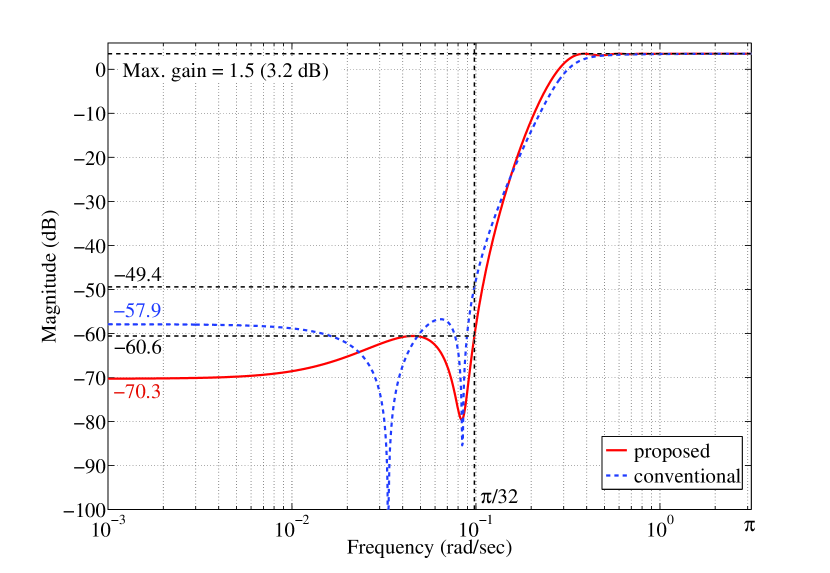
Figure 11: NTF’s: proposed (solid) and the NTF zero optimization (dash).

Then we run a simulation to evaluate the obtained modulators. We used MATLAB functions simulateDSM and simulateSNR in the Delta-Sigma Toolbox. Fig. 12 shows the spectrum of the output when the input is the sinusoidal wave with frequency 0.0325 (rad/sec) and amplitude 0.5. We assume a uniform quantizer with $M=1$ and $\delta=1/2$ (see Assumption 2). We observe that the quantization noise is well attenuated in both cases. Note that the frequency 0.0325 (rad/sec) is taken around the first notch of the conventional NTF gain (see Fig. 11). The notch frequency is expected to give much better performance to the conventional modulator than the proposed modulator. However, the simulation shows this does not necessarily hold. In fact, the peak-to-peak SNR, $\mathrm{SNR}_{\text{pp}}$ defined in (7), of our modulator is 95.5 (dB), while that of the conventional modulator is 91.5 (dB). That is, our design is superior to the conventional one in $\mathrm{SNR}_{\text{pp}}$ by approximately 4.0 (dB).

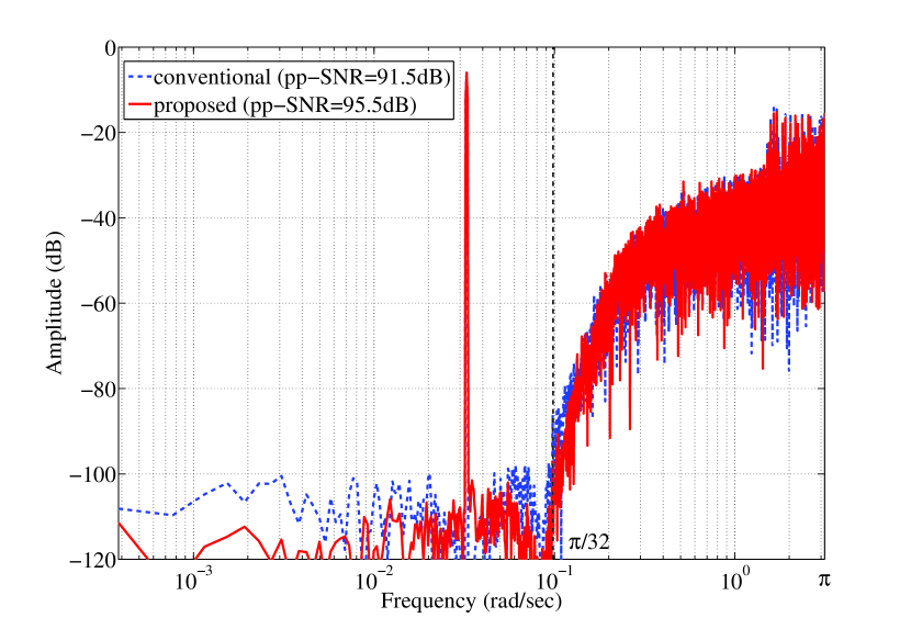
Figure 12: The spectrum of the output of the $\Delta\Sigma$ modulators: proposed (solid) and conventional (dash), pp-SNR denotes the peak-to-peak SNR.

Fig. 13 shows the SNR, the ratio of the signal power to the quantization noise power (SQNR), of the modulators as a function of the amplitude of the input sinusoidal wave with the frequency 0.0325 (rad/sec). For almost all amplitudes, the proposed modulator shows better performance than the conventional one, in particular, the difference of the peak SNR, or the maximum SNR is about 4.8 (dB).

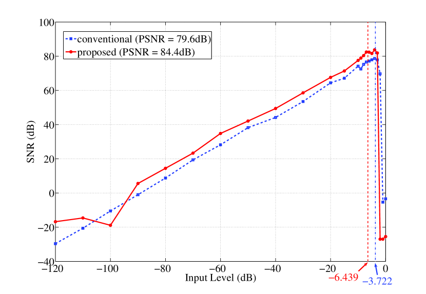
Figure 13: The SNR versus the amplitude of the input: proposed (solid) and conventional (dash). -6.439 is the stability bound for the proposed modulator, and -3.722 is for the conventional modulator.

The figure also shows the stability bounds estimated by inequality (22) in Theorem 4. That is, the bound for the conventional modulator is given by $M+1-\delta\|r\|_{1}\approx 0.6514$ (-3.722 dB), and that for the proposed modulator is $M+1-\delta\|r\|_{1}\approx 0.4765$ (-6.439 dB). The degradation of the SNR for high input levels is due to saturation in the quantizer that leads to instability in the modulator. We can say that if the input level is limited to the stability bound, the degradation is avoidable. We note that the conventional modulator can accept higher level of inputs. To see the difference more precisely, we show an enlarged plot in Fig. 14. The difference however does not matter if the inputs are limited to the pre-estimated bound by Theorem 4.

Figure 14: Enlarged plot of Fig. 13 with linear scale for input levels.

These simulation results show that the proposed min-max (or worst-case) design gives a better SNR as mentioned in Section III-A. We summarize the results in Table II.

TABLE II: Comparison in Figs. 11–13.

	max NTF (dB)	$\mathrm{SNR}_{\text{pp}}$ (dB)	peak SNR (dB)
Conventional	-49.4	91.5	79.6
Proposed	-60.6	99.5	84.4
Improvement	11.2	4.0	4.8

VI-B Bandpass modulator

We next show a design example of a bandpass modulator. We set $P(z)=1$, and $R(z)$ be an FIR filter with 32 taps. The center frequency $\omega_{0}$ is set to be $\pi/2$, and the bandwidth parameter $\Omega$ is $\pi/16$. The FIR filter $R(z)$ is designed by using the LMI in Theorem 2, with the stability condition $\|T_{\text{\rm NTF}}\|_{\infty}<1.5$. We design two modulators, with zeros at $\omega_{0}=\pm\pi/2$ and without assignment of zeros there. We also design a modulator by the NTF zero optimization [22, 2], designed by the MATLAB function synthesizeNTF in the Delta-Sigma Toolbox, with the order of $T_{\text{\rm NTF}}$ is 6, the over sampling ratio $N_{\text{OSR}}$ is 16, the center frequency $f_{0}=1/4$, and $\|T_{\text{\rm NTF}}\|_{\infty}<1.5$.

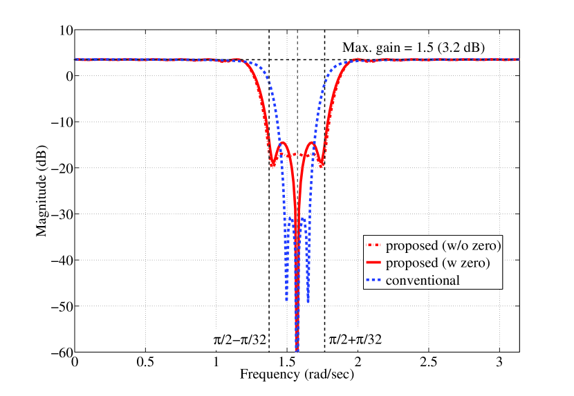
Figure 15: Bandpass NTF’s: proposed with zeros at $\omega_{0}=\pm\pi/2$ (solid), proposed without assignment of zeros (dash-dots) and the NTF zero optimization (dash).

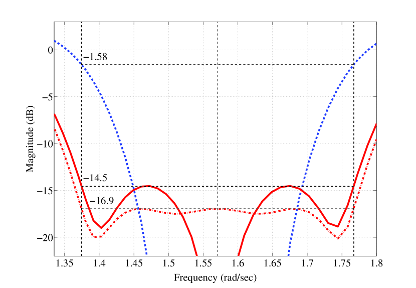
Figure 16: Enlarged view of bandpass NTF’s in Fig. 15.

Fig. 15 shows the frequency responses of the two proposed modulators and that by optimizing the NTF zeros. We can see that the proposed modulator without assignment of zeros shows the smallest magnitude over the band $[\pi/2-\pi/16,\pi/2+\pi/16]$, and that of the proposed modulator with a zero at $\pi/2$ is slightly larger. To see these precisely, enlarged figure of Fig. 15 around the center frequency is shown in Fig. 16. By this figure, the magnitudes of the proposed NTF’s are uniformly attenuated over the band, while the conventional one shows a peak on the edges of the band. The differences between the magnitudes of the proposed NTF’s and that of the conventional one are about 12.9 (dB) and 15.3 (dB).

Finally, we give an example of a multi-band modulator proposed in Section III-C. We set $P(z)=1$, and $R(z)$ be an FIR filter with 32 taps. The center frequencies are set by $\omega_{1}=\pi/4$, $\omega_{2}=\pi/2$, and $\omega_{3}=3\pi/4$. The bandwidth parameter is $\Omega_{l}=\pi/16$, $l=1,2,3$. We also impose the infinity norm condition $\|T_{\text{\rm NTF}}\|<1.5$ and place zeros at $\omega_{1}$, $\omega_{2}$, and $\omega_{3}$. Fig. 17 shows the magnitude frequency response of the NTF designed via Theorem 3.

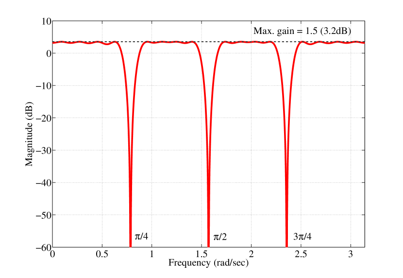
Figure 17: Multi-band bandpass NTF designed by Theorem 3 with zeros at $\omega_{1}=\pi/4$, $\omega_{2}=\pi/2$, and $\omega_{3}=3\pi/4$.

The figure shows that our design method works well.

VII Conclusion

We have proposed a min-max design method of $\Delta\Sigma$ modulators. First we have characterized all stabilizing loop-filters for a linearized model. Then, based on this result, we have formulated our problem of noise shaping in the frequency domain as a min-max optimization. It is seen that the proposed min-max design has an advantage in improving SNR.

The proposed design problem is reduced to an LMI optimization, using the generalized KYP lemma, and this has a computational advantage. The assignment of NTF zeros can be taken care of by an LME. We have given a stability analysis of the $\Delta\Sigma$ modulator model without linearization and derived an $H^{\infty}$-norm condition for stability, which is also described as an LMI via the KYP lemma. The obtained NTF is an FIR filter, which is favorable from the implementation viewpoint. Design examples have shown effectiveness of our method.

Future work includes STF optimization as in [23], or adaptive quantization as in [51] combined with the proposed optimal filter.

References

- [1] S. R. Norsworthy, R. Schreier, and G. C. Temes, Delta-Sigma Data Converters. IEEE Press, 1997.
- [2] R. Schreier and G. C. Temes, Understanding Delta-Sigma Data Converters. Wiley Interscience, 2005.
- [3] E. Janssen and D. Reefman, “Super-audio CD: An introduction,” IEEE Signal Process. Mag., vol. 20, no. 4, pp. 83–90, 2003.
- [4] U. Zölzer, Digital Audio Signal Processing, 2nd ed. John Wiley & Sons, 2008.
- [5] K. Vleugels, S. Rabii, and B. A. Wooley, “A 2.5-V sigma-delta modulator for broadband communicatinos applications,” IEEE J. Solid-State Circuits, vol. 36, no. 12, pp. 1887–1899, 2001.
- [6] A. Rusu, B. Dong, and M. Ismail, “Putting the “FLEX” in flexible mobile wireless radios,” IEEE Circuits Devices Mag., vol. 22, no. 6, pp. 24–30, 2006.
- [7] U. Gustavsson, T. Eriksson, and C. Fager, “Quantization noise minimization in modulation based RF transmitter archtectures,” IEEE Trans. Circuits Syst. I, vol. 57, no. 12, pp. 3082–3091, Dec. 2010.
- [8] I. Daubechies and R. DeVore, “Approximating a bandlimited function using very coarsely quantized data: A family of stable sigma-delta modulators of arbitrary order,” Annals of Mathematics, vol. 158, no. 2, pp. 679–710, 2003.
- [9] J. Benedetto, A. Powell, and O. Yılmaz, “Sigma-delta quantization and finite frames,” IEEE Trans. Inf. Theory, vol. 52, no. 5, pp. 1990–2005, May 2006.
- [10] M. Lammers, A. M. Powell, and O. Yılmaz, “Alternative dual frames for digital-to-analog conversion in sigma–delta quantization,” Adv. Comput. Math., vol. 32, no. 1, pp. 73–102, Jan. 2010.
- [11] P. Boufounos and R. G. Baraniuk, “Sigma delta quantization for compressive sensing,” in Proc. SPIE Waveletts XII, vol. 6701, Aug. 2007.
- [12] C. S. Güntürk, M. Lammers, A. Powell, R. Saab, and O. Yılmaz, “Sigma delta quantization for compressed sensing,” in 44th Annual Conf. on Inf. Sci. and Syst. (CISS), 2010, pp. 1–6.
- [13] S. Azuma and T. Sugie, “Optimal dynamic quantizers for discrete-valued input control,” Automatica, vol. 44, no. 2, pp. 396–406, Feb. 2008.
- [14] ——, “Synthesis of optimal dynamic quantizers for discrete-valued input control,” IEEE Trans. Autom. Control, vol. 53, no. 9, pp. 2064–2075, Oct. 2008.
- [15] S. Callegari, F. Bizzarri, R. Rovatti, and G. Setti, “On the approximate solution of a class of large discrete quadratic programming problems by modulation: The case of circulant quadratic forms,” IEEE Trans. Signal Process., vol. 58, no. 12, pp. 6126–6139, 2010.
- [16] A. Fazel, A. Gore, and S. Chakrabartty, “Resolution enhancement in learners for superresolution source separation,” IEEE Trans. Signal Process., vol. 58, no. 3, pp. 1193–1204, Mar. 2010.
- [17] A. Gore and S. Chakrabartty, “A min–max optimization framework for designing learners: Theory and hardware,” IEEE Trans. Circuits Syst. I, vol. 57, no. 3, pp. 604–617, Mar. 2010.
- [18] F. Krahmer and R. Ward, “Lower bounds for the error decay incurred by coarse quantization schemes,” Applied and Computational Harmonic Analysis, vol. 32, no. 1, pp. 131–138, Jan. 2012.
- [19] T. Hayashi, Y. Inabe, K. Uchimura, and A. Iwata, “A multistage delta-sigma modulator without double integration loop,” ISSCC Digest of Technical Papers, pp. 182–183, 1986.
- [20] J. C. Candy and A. Huynh, “Double integration for digital-to-analog conversion,” IEEE Trans. Commun., vol. 34, no. 12, pp. 1746–1756, 1986.
- [21] A. Datta, M.-T. Ho, and S. P. Bhattacharyya, Structure and Synthesis of PID Controllers. Springer, 1995.
- [22] R. Schreier, “An empirical study of high-order single-bit delta-sigma modulators,” IEEE Trans. Circuits Syst. II, vol. 40, no. 8, pp. 461–466, 1993.
- [23] C.-F. Ho, B. Ling, J. Reiss, Y.-Q. Liu, and K.-L. Teo, “Design of interpolative sigma delta modulators via semi-infinite programming,” IEEE Trans. Signal Process., vol. 54, no. 10, pp. 4047–4051, Oct. 2006.
- [24] M. Nagahara, T. Wada, and Y. Yamamoto, “Design of oversampling delta-sigma DA converters via optimization,” in Proc. of IEEE ICASSP, vol. III, 2006, pp. 612–615.
- [25] M. Nagahara, “Min-max design of FIR digital filters by semidefinite programming,” in Applications of Digital Signal Processing. InTech, Nov. 2011, pp. 193–210.
- [26] Y. Yamamoto, M. Nagahara, and P. P. Khargonekar, “Signal reconstruction via sampled-data control theory—Beyond the Shannon paradigm,” IEEE Trans. Signal Process., vol. 60, no. 2, pp. 613–625, Feb. 2012.
- [27] T. Parks and J. McClellan, “Chebyshev approximation for nonrecursive digital filters with linear phase,” IEEE Trans. Circuit Theory, vol. 19, no. 2, pp. 189–194, Mar. 1972.
- [28] M. Nagahara and Y. Yamamoto, “Optimal noise shaping in delta-sigma modulators via generalized KYP lemma,” in Proc. of IEEE ICASSP, 2009, pp. 3381–3384.
- [29] ——, “Optimal design of delta-sigma modulators via generalized KYP lemma,” in Proc. of ICROS-SICE International Joint Conference, 2009, pp. 4376–4379.
- [30] T. Iwasaki and S. Hara, “Generalized KYP lemma: unified frequency domain inequalities with design applications,” IEEE Trans. Autom. Control, vol. AC-50, pp. 41–59, 2005.
- [31] D. Quevedo and G. Goodwin, “Multistep optimal analog-to-digital conversion,” IEEE Trans. Circuits Syst. I, vol. 52, no. 3, pp. 503–515, Mar. 2005.
- [32] J. Østergaard, D. Quevedo, and J. Jensen, “Real-time perceptual moving-horizon multiple-description audio coding,” IEEE Trans. Signal Process., vol. 59, no. 9, pp. 4286–4299, Sep. 2011.
- [33] S.-H. Yu, “Analysis and design of single-bit sigma-delta modulators using the theory of sliding modes,” IEEE Trans. Control Syst. Technol., vol. 14, no. 2, pp. 336–345, Mar. 2006.
- [34] F. Yang and M. Gani, “An approach for robust calibration of cascaded sigma–delta modulators,” IEEE Trans. Circuits Syst. I, vol. 55, no. 2, pp. 625–634, Mar. 2008.
- [35] J. McKernan, M. Gani, F. Yang, and D. Henrion, “Optimal low-frequency filter design for uncertain 2-1 sigma-delta modulators,” IEEE Signal Process. Lett., vol. 16, no. 5, pp. 362–365, May 2009.
- [36] M. Osqui, M. Roozbehani, and A. Megretski, “Semidefinite programming in analysis and optimization of performance of sigma-delta modulators for low frequencies,” in Proc. of the American Control Conf., 2007, pp. 3582–3587.
- [37] A. Teplinsky, E. Condon, and O. Feely, “Driven interval shift dynamics in sigma-delta modulators and phase-locked loops,” IEEE Trans. Circuits Syst. I, vol. 52, no. 6, pp. 1224–1235, Jun. 2005.
- [38] C. S. Güntürk and N. T. Thao, “Refined error analysis in second-order modulation with constant inputs,” IEEE Trans. Inf. Theory, vol. 50, no. 5, pp. 839–860, May 2004.
- [39] C. Y.-F. Ho, B. W.-K. Ling, J. D. Reiss, and X. Yu, “Global stability, limit cycles and chaotic behaviors of second order interpolative sigma delta modulators,” International Journal of Bifurcation and Chaos, vol. 21, no. 6, pp. 1755–1772, 2011.
- [40] S. Boyd, L. E. Ghaoui, E. Feron, and V. Balakrishnan, Linear Matrix Inequalities in System and Control Theory. SIAM, 1994.
- [41] Y. Yamamoto, B. D. O. Anderson, M. Nagahara, and Y. Koyanagi, “Optimizing FIR approximation for discrete-time IIR filters,” IEEE Signal Process. Lett., vol. Vol. 10, No. 9, 2003.
- [42] J. Löfberg, “YALMIP : A toolbox for modeling and optimization in MATLAB,” in Proc. IEEE International Symposium on Computer Aided Control Systems Design, 2004, pp. 284–289. [Online]. Available: http://users.isy.liu.se/johanl/yalmip/
- [43] J. F. Sturm, “Using SeDuMi 1.02, a MATLAB toolbox for optimization over symmetric cones,” 2001. [Online]. Available: http://sedumi.ie.lehigh.edu/
- [44] S. Boyd and L. Vandenberghe, Convex Optimization. Cambridge University Press, 2004.
- [45] S. Jantzi, R. Schreier, and M. Snelgrove, “Bandpass sigma-delta analog-to-digital conversion,” IEEE Trans. Circuits Syst., vol. 38, no. 11, pp. 1406–1409, Nov. 1991.
- [46] S. Jantzi, K. Martin, and A. Sedra, “Quadrature bandpass modulation for digital radio,” IEEE J. Solid-State Circuits, vol. 32, no. 12, pp. 1935–1950, Dec. 1997.
- [47] J. G. Kenney and L. R. Carley, “Design of multibit noise-shaping data converters,” Analog Int. Circuits Signal Processing Journal, vol. Vol. 3, pp. 259–272, 1993.
- [48] M. A. Dahleh and I. J. Diaz-Bobillo, Control of Uncertain Systems. Prentice Hall, 1995.
- [49] K. C. H. Chao, S. Nadeem, W. L. Lee, and C. G. Sodini, “A higher order topology for interpolative modulators for oversampling A/D conversion,” IEEE Trans. Circuits Syst., vol. 37, no. 3, pp. 309–318, 1990.
- [50] R. Schreier, “Delta sigma toolbox.” [Online]. Available: http://www.mathworks.com/matlabcentral/fileexchange/19
- [51] J. Østergaard and R. Zamir, “Multiple-description coding by dithered delta-sigma quantization,” IEEE Trans. Inf. Theory, vol. 55, no. 10, pp. 4661–4675, Oct. 2009.
- [52] J. C. Doyle, B. A. Francis, and A. R. Tannenbaum, Feedback Control Theory. Maxwell Macmillan, 1992.
- [53] Mathworks, “Control system toolbox users guide,” 2010. [Online]. Available: http://www.mathworks.com/products/control/