Calibrated Estimates of the Energy in Major Flares of GRS 1915+105

Abstract

We analyze the energetics of the major radio flare of October 8 2005 in GRS 1915+105. The flare is of particular interest because it is one of the most luminous and energetic radio flares from a Galactic black hole that has ever been observed. The motivation is two-fold. One, to learn more about the energetics of this most extreme phenomenon and its relationship to the accretion state. The second is to verify if the calibrated estimates of the energy of major radio flares (based on the peak low frequency optically thin flux) derived from flares in the period 1996-2001 in Punsly & Rodriguez (2013), PR13 hereafter, can be used to estimate plasmoid energy beyond this time period. We find evidence that the calibrated curves are still accurate for this strong flare. Furthermore, the physically important findings of PR13 are supported by the inclusion of this flare: the flare energy is correlated with both the intrinsic bolometric X-ray luminosity, $L_{\mathrm{bol}}$, $\sim 1$ hour before ejection and $L_{\mathrm{bol}}$ averaged over the duration of the ejection of the plasmoid and $L_{\mathrm{bol}}$ is highly elevated relative to historic levels just before and during the ejection episode. A search of the data archives reveal that only the October 8 2005 flare and those in PR13 have adequate data sampling to allow estimates of both the energy of the flare and the X-ray luminosity before and during flare launch.

1 Introduction

Accretion and the associated ejection processes are ubiquitous phenomena of our Universe. They are indeed seen in many astrophysical objects: they power the distant gamma-ray bursts, the massive black holes lurking at the center of active galaxies. Closer to us accretion/ejection is also a source of radiations in young stellar objects and in Galactic accreting compact objects also referred to as ’microquasars’. Understanding the physics of accretion and jets and also their (potential) links is thus of primal importance to understand a large range of celestial objects. In this respect microquasars present several advantages over the other aforementioned sources. They are close and (very) bright in most wavelengths which makes them easy to observe and follow, and they also vary on short human-followable time scales (from ms to year).

The black hole GRS 1915+105 launches more superluminal radio flares out to large distances than any other Galactic object (Mirabel & Rodriguez, 1994; Fender et al, 1999; Dhawan et al, 2000). The incredibly large energy of the major ejections pushes our understanding of the physics of jet launching in black hole accretion systems to the limit. Great progress was made towards establishing phenomenological relationships between the accretion flow before and during flare launch and the power of the relativistic ejections in Punsly & Rodriguez (20131a, PR13 hereafter). However, our understanding is far from complete. The most energetic radio flares are the most enigmatic from a physical perspective. It is very unclear how an accretion flow around a black hole can eject so much energy (Punsly & Rodriguez, 2013b). Very strong radio flares ($\sim$ the Eddington luminosity) are rare and few of these have information regarding the accretion flow from serendipitous X-ray observations just before and during the ejection process.

Microquasars exhibit two distinct types of jets: discrete ejections of ’plasmoids’ Mirabel & Rodriguez (1994), the major flares that are the subject of this study, and the so-called compact jet that is present during the X-ray hard state (Corbel et al, 2000, 2003; Gallo et al, 2003). There is no established relationships between these two outflow states and the physical connection between the two phenomena, if any, is not well understood. Huge multi-wavelength efforts have been made in the past twenty years to try and understand the origin of all type of jets and their connection to the accretion processes (e.g. Mirabel et al (1998); Corbel et al (2000, 2003); Klein-Wolt et al. (2001); Gallo et al (2003); (2008a, b, 2010)). Still, the physical relationship between the accretion flow and the production of jetted outflows remans speculative. This is especially so for the powerful major ejections. In PR13, it was pointed out that X-ray observations with time resolution on the order of days are too coarsely spaced to resolve the X-ray state before and during the brief major flare ejection episodes that occur unexpectedly a few times a year. As a consequence, any X-ray data that is coincident with the instant of major ejection launching is purely serendipitous. Culling through large RXTE data sets, it was demonstrated in PR13 that empirical relationships exist between the accretion states and major flare ejections. In particular, the X-ray luminosity is highly elevated in the last hours preceding major ejections and it is correlated with the power required to eject the discrete plasmoids. Secondly, the X-ray luminosity was found to be highly variable during the ejection of the plasmoids, but the time averaged X-ray luminosity during the ejection event is correlated with that just before the plasmoid is launched and is of a similar (but perhaps a slightly lower) level. Thusly motivated, we seek to expand the database of PR13 that showed the correlated disk-jet behavior.

In this paper, we study one such extremely powerful major radio flare, that of October 8 2005 (MLD 53651). We estimate that is the fifth or sixth strongest radio flare ever detected in the 20 years of monitoring GRS 1915+105. Of these 6 radio flares only this flare and the radio flare launched on April 13 1998 (MJD 50916) have X-ray observations just before and during the launching of the ejection. This strong radio flare provides an excellent test case to validate the empirical relationships between the accretion state before and during radio flare launch and the energy of the major radio flare that were found in PR13. The paper is organized as follows. Section 2 describes the estimation of the radio flare ejection time. Section 3 is an estimate of the intrinsic X-ray luminosity from 1.2 keV - 50 keV, $L_{\mathrm{bol}}$, before and during the launch of the plasmoid. The following section is a computation of the energy of the plasmoid, $E$, associated with the radio flare. Section 5 will compare the results of Sections 3 and 4 to the empirical relationships in PR13.

2 The Time of Ejection Launch

Determining the time of the ejection is essential. It allows us to establish a temporal (and perhaps causal) chain of events and the fluence. This time signature provides a physical context for the individual X-ray observations. Every optically thin radio flare is preceded by a rise in optically thick high frequency radio emission. As the ejected plasmoid expands, the optical depth to synchrotron self absorption (SSA) decreases and the spectrum steepens at ever decreasing frequency until it is optically thin at low frequency. In PR13 it was shown that the 15 GHz light curve (from the Ryle Telescope public archive http://www.mrao.cam.ac.uk/ guy/1915/) can provide an excellent estimate of the time that the plasmoids were ejected. This is true provided that the linear extrapolation of the light curve backwards in time to the background flux density level is sufficiently short. This was verified both empirically by the agreement of this technique with plasmoid ejections times deduced from radio interferometry data and also with theoretical arguments in PR13. One reason for choosing the radio flare on MJD 53651 (MJD will be dropped hereafter) is the excellent launch time estimate, the details of which are illustrated in Figure 1. We have no estimate of the background flux density level because GRS 1915+105 was very active preceding this radio flare. However, the rise is very steep and to a very high level. Thus, inspection of Figure 1 indicates that the only plausible extrapolations to a nonzero background flux level yields a start time between 53650.78 and 5360.83 (a mere 1 hour uncertainty).

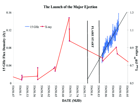
Figure 1: A detailed view of the 15 GHz flux density and the intrinsic X-ray luminosity, $L_{\mathrm{bol}}$, light curves near the estimated ejection time for the MJD 53651 radio flare. $L_{\mathrm{bol}}$ is estimated from the RXTE ASM data per the methods of PR13 as detailed in Section 3.

3 The Intrinsic X-ray Luminosity

An important result from PR13 was the development and validation of a method to estimate the intrinsic X-ray luminosity from 1.2 keV - 50 keV, $L_{\mathrm{bol}}$, from the ASM data of RXTE. The estimates of $L_{\mathrm{bol}}$ are based on models where the main contribution is due to thermal Comptonisation of soft (cold $\sim 0.2$ keV) photons by hot ($\sim$ 20-100 keV) electrons present in a so-called corona. The important parameters to estimate $L_{\mathrm{bol}}$ are $\mathrm{kT_{inj}}$, $\mathrm{kT_{e}}$, $\tau$ and the Comptonised normalization (see Section 4.2.2 of PR13). The method was verified by finding PCA observations that are modeled as such and comparing them to quasi-simultaneous ASM data. The estimator was derived using $\chi$ class spectra as defined by Belloni et al (2000), but empirically the estimator applies fairly accurately to all the PCA models of states that it was tested against except the very soft states. Comparison to the PCA generated models indicate a very small stochastic relative error of 13% - 14%. The main systematic error in $L_{\mathrm{bol}}$ is in the column density, $N_{H}$, to the source. From Belloni et al (1997); Muno et al (1999) we expect a systematic error less than a factor of 2 arising from the uncertainty in $N_{H}$, too small to affect our conclusions. Our estimator from PR13 is included in the Appendix for convenience.

4 The Energy of the Ejection

It was determined in Punsly (2012, P12), that knowledge of the time evolution of the spectral shape associated with a changing SSA opacity (defined from the center of the plasmoid along a line of sight to Earth), $\tau$, greatly enhances the accuracy of plasmoid energy, $E$, estimates because it constrains the size. The frequency and the width of the spectral peak provide two added pieces of information at each epoch of observation beyond the single epoch spectral index and flux density that is traditionally used to estimate the ejected $E$ (Fender et al, 1999; Mirabel & Rodriguez, 1994). The slowly evolving SSA opacity of the powerful radio flares of December 1993 was considered in the context baryon number conservation, energy conservation, synchrotron cooling times and X-ray luminosity in P12 to eliminate uncertainty in the energy estimates. Namely,

1. The evolving $\tau$ restricts the total column depth and plasma-filled volume, which ameliorates issues associated with filling factor that occur in a more simplified typical minimum energy analysis.

2. A near minimum energy condition is shown to occur when the optically thin low frequency emission is near maximum based on the constraint of energy conservation and the synchrotron cooling times of a plasmoid with an evolving $\tau$ (see Section 5 and Figure 14 of P12). The peak occurs when the optical depth at 2.3 GHz, $\tau_{2.3}$, $\approx 0.1$.

3. Baryon number conservation and synchrotron cooling times in combination with the evolving $\tau$ indicate that a large protonic component requires the jet to begin nonmagnetic with most of the energy in mechanical form (see Section 4 and Figures 12 and 13 of P12). Yet there is insufficient radiation or thermal pressure to initiate this outflow. Thus, only the leptonic dominated branch in solution space can be integrated back to the source. These begin magnetically dominated and magnetic energy is converted to mechanical energy as equipartition is approached.

4. The magnitude of the 1.4 GHz emission requires that the energy spectrum of electrons extend to a minimum energy, $U_{min}<6m_{e}c^{2}$ (see Section 5 of P12).

In summary, the proton content is minimal, the plasmoid attains a near minimum energy condition, $\tau_{2.3}\approx 0.1$ and $U_{min}\approx m_{e}c^{2}$, when the optically thin flux at 2.3 GHz, $S_{\mathrm{thin}}(2.3)$, is near maximum. As in n PR13 we invoke one assumption: the detailed modeling of the time evolution of the radio flares from P12 can be used as a template for the time evolution of other plasmoids with less supporting data. In this study, we have the advantage of the complete spectral shape including the SSA turnover. So it is possible to solve for $\tau_{2.3}$ at the epoch of observation. Thus, this calculation is more accurate than those of PR13 for which complete spectral data does not exist.

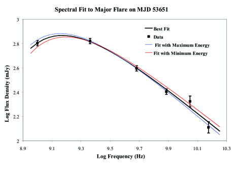
Figure 2: Fits to the RATAN-600 data on MJD 53651 after core flux subtraction. The Ryle 15 GHz data is one day after that in Figure 1.

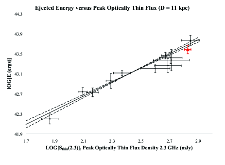
Figure 3: The energy, E, estimate derived here for the 53651 radio flare (red diamond) from the complete spectrum in Figure 2 compared to the empirical fit from Punsly and Rodriguez (2013b) of $E$ versus the peak $S_{\mathrm{thin}}(2.3)$, the black data points. The linear least squares fit with uncertainty in both variables is $\log[E(\mathrm{ergs})]=(39.69\pm 0.24)+(1.41\pm 0.09)\log[S_{\mathrm{thin}}(2.3)/1\mathrm{mJy}]$. The dashed lines result from combinations of the minimum and maximum fitted values of the coefficients as in Reed (1988) and represent the steepest and flattest fits consistent with the data.

Except when noted, a fiducial distance to GRS 1915+105 of D =11 kpc is assumed throughout the manuscript. However, we consider every plausible value of D and the corresponding dependent Doppler factor, $\delta$, because of the large systematic uncertainty in $\delta$. The Doppler factor is given in terms of $\overline{\Gamma}$, the Lorentz factor of the outflow; $\beta$, the three velocity of the outflow and the angle of propagation to the line of sight, $\theta$; $\delta=1/[\overline{\Gamma}(1-\beta\cos{\theta})]$ (Lind & Blandford, 1985). In order to estimate $\delta$ from D, we assume that the kinematic results from Fender et al (1999) are common to the entire time frame from 1997 to 2005 as evidenced by interferometric observations of multiple radio flares Dhawan et al (2000); Miller-Jones et al (2005). The intrinsic flux density is $S_{\mathrm{thin}}(2.3)\delta^{-(3+\alpha)}$. As D is varied from 10.5 kpc to near the maximum kinematically allowed value of 11 kpc, the intrinsic spectral luminosity changes by a factor $\approx(11/10.5)^{2}(0.33/0.56)^{4}=(1/7.5)$ which equates to a reduction of $E$ by a factor $\sim$ 5 - 6.

Figure 2 shows the spectrum from RATAN-600 data provided by S. Trushkin (private communication 2013). In addition there is a 15 GHz data point from the Ryle archives. Before fitting the data, we want to extract the spectrum of the ejected plasmoid from the flat spectrum core. The method from Section 3.2 of PR13 assumes that the random variations in the 15 GHz light curve that occur after the radio flare has risen to its peak represent optically thick time variations of the core. This estimation is computed by first performing a linear fit to the 15 GHz flux density from 56351.62 to 56351.91 (a day after the data presented in Figure 1). The magnitude of the standard deviation of the residuals from the linear fit to the data (15 mJy) is considered to be the time averaged radio core flux density at 15 GHz (flat spectrum: $\alpha=0$ is assumed). For such a strong radio flare this is just a small pedantic refinement.

We fitted the spectral energy distribution (SED) by the methods described by Equations (1-6). We find three fits to the data by minimizing $\chi^{2}$. The black curve is the nominal fit to the data points. This best fit is a powerlaw spectral luminosity with spectral index $\alpha=0.98$ that is transferred through an SSA opacity with $\tau_{2.3}=0.33$. The blue curve represents the fit which has the maximum plasmoid energy, it uses the maximum value of the flux density at 1 GHz and 2.3 GHz (top of the error bars) and the minimum value of the flux density (bottom of the error bars) at the high frequency points. This fit has $\alpha=1.03$ and $\tau_{2.3}=0.35$. The red curve represents the fit which has the minimum plasmoid energy, it uses the minimum value of the flux density at 1 GHz and 2.3 GHz and the maximum value of the flux density at the high frequency points. This fit has $\alpha=0.94$ and $\tau(2.3)=0.33$. Using the nominal value and the maximum and minimum fits, one can compute self consistent solutions to the Equations (1- 6) in P12 and below.

The relationships are expressed in observed quantities designated with a subscript, “o”. Taking the standard result for the SSA attenuation coefficient in the plasma rest frame and noting that the frequency obeys $\nu=\nu_{o}/\delta$, from (1996); Ginzburg & Syrovatskii (1969)

$$\mu(\nu)=\frac{3^{\alpha+1}\pi^{0.5}g(p)e^{2}N_{\Gamma}}{8m_{e}c}\left(\frac{eB}{m_{e}c}\right)^{(1.5+\alpha)}\left(\frac{\delta}{\nu_{o}}\right)^{(2.5+\alpha)}$$ (1)

$$g(n)=\frac{\Gamma[(3n+22)/12]\Gamma[(3n+2)/12]\Gamma[(n+6)/4]}{\Gamma[(n+8)/4]}\;.$$ (2)

This equation derives from an assumed powerlaw energy distribution for the relativistic electrons, $N(U)=N_{\Gamma}U^{-n}$, where the radio spectral index $\alpha=(n-1)/2$ and $U$ is the energy of the electrons in units of $m_{e}c^{2}$. The radiative transfer equation was solved in Ginzburg & Syrovatskii (1969) to yield the following parametric form for the observed flux density, $S_{\nu}$, from the SSA source,

$$(S_{\nu})_{o}=\frac{S_{1}\nu^{-\alpha}}{R\mu(\nu)}\times\left(1-e^{-\mu(\nu)R}\right)\;,$$ (3)

where R is the radius of the spherical region in the rest frame of the plasma and $S_{1}$ is a normalization factor. In the spherical, homogeneous approximation, one can make a simple parameterization of the SSA attenuation coefficient, $\mu(SSA)=\mu_{1}\nu_{o}^{-(2.5+\alpha)}$. If one assumes that the source is spherical and homogeneous then there are three unknowns in Equation (3), $R\mu_{1}$, $\alpha$ and $S_{1}$; $(S_{\nu})_{o}$ is determined by observation. There is a finite range of physical parameters that are consistent with these spectral fits. To make the connection, one needs to relate the observed flux density in Equation (3) to the local synchrotron emissivity within the plasma. The synchrotron emissivity is given in Tucker (1975),

$$j_{\nu}=1.7\times 10^{-21}(4\pi N_{\Gamma})a(n)B^{(1+\alpha)}(4\times 10^{6}/\nu)^{\alpha}\;,$$ (4)

$$a(n)=\frac{\left(2^{\frac{n-1}{2}}\sqrt{3}\right)\Gamma\left(\frac{3n-1}{12}\right)\Gamma\left(\frac{3n+19}{12}\right)\Gamma\left(\frac{n+5}{4}\right)}{8\sqrt{\pi}(n+1)\Gamma\left(\frac{n+7}{4}\right)}\;.$$ (5)

One can transform this to the observed flux density, $(S_{\nu}(\nu_{o}))_{o}$, in the optically thin region of the spectrum using the relativistic transformations from Lind & Blandford (1985),

$$(S_{\nu}(\nu_{o}))_{o}=\frac{\delta^{(3+\alpha)}}{4\pi D^{2}}\int{j_{\nu}^{{}^{\prime}}dV{{}^{\prime}}}\;,$$ (6)

where $j_{\nu}^{{}^{\prime}}$ is evaluated in the plasma rest frame at the observed frequency.

Solving Equations (1-6) simultaneously yields an infinite number of solutions for a given D and $\delta$ that are parameterized by $\tau$, $R$, $N_{\Gamma}$ and $B$. Assuming that $S_{\mathrm{thin}}(2.3)=675\;\mathrm{mJy}$ (Figure 2) is near the peak $S_{\mathrm{thin}}(2.3)$ (based on its large value and the steep spectral index at higher frequencies), according to finding ii) above from P12, the solution with minimum energy will be close to the physical solution. Using this insight to compute the energy corresponding to the three fits in Figure 2 yields the (Earth frame) energy for $D$ = 11 kpc, $\delta=0.33$ and $\overline{\Gamma}=5.0$ (see Fender et al (1999)),

$$E=(3.84\pm 0.82)\times 10^{43}\mathrm{ergs}\;.$$ (7)

Similar expression can be found for other values of $D$ (as in PR13). The corresponding $\delta$ and $\overline{\Gamma}$ can be determined from the kinematics derived from interferometric measurements per the methods of Fender et al (1999).

Figure 3 compares the value of $E$ in Equation (7) to that expected from a peak $S_{\mathrm{thin}}(2.3)=675\;\mathrm{mJy}$ based on the best fit estimator from Punsly & Rodriguez (2013b). The fit to the data is by the method of list least squares with uncertainty in both variables Reed (1989). The dashed lines result from combinations of the minimum and maximum fitted values of the coefficients as in Reed (1989) and represent the steepest and flattest fits consistent with the data. The radio flare on 53651 lies just below the curve but within 1 $\sigma$ uncertainty. This is expected from the conclusions of P12 noted in finding ii): the plasmoid should approach minimum energy at $\tau_{2.3}\approx 0.1$, but $\tau_{2.3}=0.33-0.35$ in the spectral fits. Consequently, if the results of P12 are appropriate then the plasmoid has not quite reached a minimum energy configuration during the observation and the energy should be slightly elevated above minimum energy. This is consistent with Figure 3, if the energy were slightly elevated, the data would lie closer to the fitted curve from Punsly & Rodriguez (2013b).

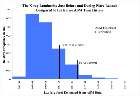
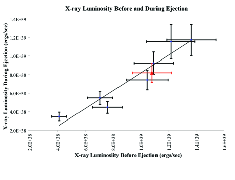
Figure 4: The top frame shows a histogram of the historic distribution of $L_{\mathrm{bol}}$ based on $>76,000$ ASM observations. The elevated levels of $L_{\mathrm{pre-flare}}$ and $L_{\mathrm{rise}}$ for the 53651 radio flare are indicated by the black vertical lines. The red diamond in the bottom frame shows that $L_{\mathrm{pre-flare}}$ and $L_{\mathrm{rise}}$ for the 53651 radio flare obey the same correlation determined by the radio flares from PR 13 in black. The linear fit is $L_{\mathrm{rise}}=0.96L_{\mathrm{pre-flare}}-1.39\times 10^{38}\mathrm{ergs/sec}$.

5 Comparison to the Results of PR13

The top frame in Figure 4 shows that the X-ray luminosity from Figure 1 is elevated just (less than 4 hours) before ejection, $L_{\mathrm{pre-flare}}$, and also so is the time average X-ray luminosity during ejection, $L_{\mathrm{rise}}$, relative to the historical distribution of $L_{\mathrm{bol}}$ as was shown for other strong radio flares in PR13 (the ASM historical distribution is from Figure 16 of PR13). The bottom frame of Figure 4 shows that the data for the 53651 radio flare follows the trend of other radio flares noted in Table 5 of PR13, $L_{\mathrm{pre-flare}}$ is highly correlated with $L_{\mathrm{rise}}$.

Figure 5 plots the 56351 radio flare data on the background of the correlations of E with $L_{\mathrm{pre-flare}}$ and $L_{\mathrm{rise}}$ from PR13. Figure 5 indicates that these potentially important physical connections between the ejection and the accretion state gain further support from the particular case of 53651. The radio flare was not included in PR13 because there is no 15 GHz coverage to indicate the end of the plasmoid ejection episode, so we cannot estimate the power required to launch the plasmoid, $Q$ - a necessary condition for inclusion in PR13. Thus, we cannot explore the correlations with $Q$ and other parameters here.

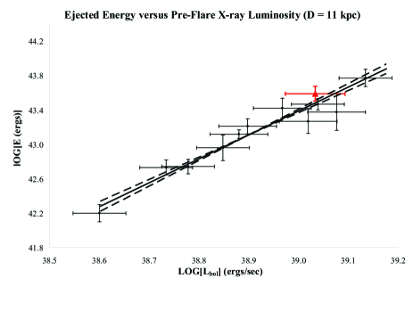
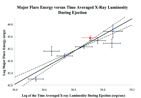
Figure 5: The top (bottom) frame illustrates the correlation between E and $L_{\mathrm{pre-flare}}$ ($L_{\mathrm{rise}}$). The data point for 53651 is a red diamond and the fit by the method of least squares with uncertainty in both variables is from the data in PR13 in black. The dashed lines result from combinations of the minimum and maximum fitted values of the coefficients as in Reed (1988) and represent the steepest and flattest fits consistent with the data. The empirical fits are $\log[E(\mathrm{ergs})]=-(65.07\pm 7.76)+(2.78\pm 0.20)\log[L_{\mathrm{pre-flare}}(\mathrm{ergs/sec})]$ and $\log[E(\mathrm{ergs})]=-(61.31\pm 21.23)+(2.69\pm 0.55)\log[L_{\mathrm{rise}}(\mathrm{ergs/sec})]$. Figures 4 and 5 indicate that $L_{\mathrm{rise}}$ is a little smaller than expected from the PR13 sample.

6 Conclusion

In this paper, we explore the energy of the plasmoid responsible for the major radio flare from GRS 1915+105 on MJD 53651 and the X-ray state just before and during ejection. Comparing to the historical distribution of flare energy in Figure 2 of Punsly & Rodriguez (2013b) indicates that this is the second most energetic flare observed since 1996. The value of $E$ is slightly larger than what we estimated for the large flare of April 8, 2003 from the spectral data in Fuchs et al (2004). Due to uncertainty in the estimates, we cannot say definitively which is larger. The analysis presented here confirms the calibration of the estimator of $E$ computed from $S_{\mathrm{thin}}(2.3)$ in Punsly & Rodriguez (2013b) and in Figure 3 here. This study also provides more evidence to support the strong correlations from PR13 between E and $L_{\mathrm{pre-flare}}$ and E with $L_{\mathrm{rise}}$ (Figure 5) as well as $L_{\mathrm{pre-flare}}$ and $L_{\mathrm{rise}}$ (Figure 4). We also find more evidence of the finding of PR13 that $L_{\mathrm{pre-flare}}$ and $L_{\mathrm{rise}}$ are elevated for strong flares (Figure 4). It is important to note that the validity of the correlations is not affected by the two main systematic uncertainties, $D$ (and the implied changes to $\delta$ and $\overline{\Gamma}$) and $N_{H}$. The curves in Figures 3- 5 just shift as shown in Table 5 of PR13.

The correlations of the accretion state preceding and during major flare ejections found in PR13 and supported by the data presented here constrain the physics of the mechanism that launches superluminal plasmoids. The fact that the power of major flare ejections is correlated with an elevated X-ray luminosity combined with the fact that the X-ray luminosity of GRS 1915+105 is also one of the highest of any known microquasar, Done et al (2004), leads to the obvious speculation that GRS 1915+105 is a prolific source of major ejections as a consequence of the high emissivity of the accretion flow. Since GRS 1915+105 radiates at a significant fraction of the Eddington luminosity and it produces relativistic outflows, it is also natural to consider the hypothesis that it is a small scale radio loud quasar. In Punsly & Rodriguez (2013b), we considered this idea in the context of numerical simulations of accretion flows onto spinning black holes. We could not exclude the possibility that the ejections are driven by the accretion flow proper, but we could constrain the physics of black hole driven jets. In particular, we found:

• The high luminosity of the accretion flow before and during plasmoid launch excludes accretion states that are obstructed by an overabundance of magnetic flux since this suppresses the source of local dissipation, the magneto-rotational instability. In particular, the so-called MADs (magnetically arrested accretion) and MCAFs (magnetically choked accretion flows) that have been developed in Mckinney et al (2012) would not produce the observed high luminosity accretion flows.

• If there is an analogy to radio loud quasars then the distance to GRS 1915+105 must greater than 10.7 kpc, otherwise the time averaged ejected power is too small.

• If there is a black hole spin related explanation of the power source for the major ejections then there is only one consistent set of existing 3-D numerical solutions. These are characterized by three factors. An accretion flow that is far below the saturation point for large scale magnetic flux. Thus, the magnetic field strength near the black hole is governed by the pressure of the accretion flow. This naturally correlates the power required to launch the ejection with the accretion rate and X-ray luminosity. Secondly, large scale magnetic flux must thread the inner regions of the accretion flow in the ergosphere (the active region of the black hole geometry). This results in the ergospheric disk jet that occurs in the 3-D simulations that are described in detail in Punsly et al (2010). Thirdly, if FR II quasars are scaled up version of GRS 1915+105, the data are consistent with numerical models when they contain an ergospheric disk jet and the BH spin $a/M>0.984$. This result is intriguing because it agrees with the value of $a/M=0.99\pm 0.01$ that was estimated from a completely independent method, study based on X-ray spectra of GRS 1915+105 (McClintock et al, 2006; Blum et al, 2009).

The need for a high bolometric luminosity prior to ejection in GRS 1915+105 and the fact that this source may be a small scale FR II also opens interesting possibilities for the study of radio loud AGNs. By following the UV-X-ray activity of the latter it should then be possible to predict the onset of discrete ejection and plan follow up radio observations more easily (due to the longer time scale in AGN). This in turn could help us obtain more stringent constrains on the jet properties in different types of accreting back holes

Appendix A Estimator for $L_{bol}$

The estimator of PR13 is defined in terms of the three ASM bins, 1.2–3 keV, 3–5 keV and 5–12 keV, bin 1, bin 2 and bin 3, respectively. The counts rates in each bin are defined

$$C1\equiv\mathrm{cts/s\;in\;bin\;1}\;,$$ (8)

$$C2\equiv\mathrm{max}(5.75,\mathrm{cts/s\;in\;bin\;2})\;,$$ (9)

$$C3\equiv\mathrm{cts/s\;in\;bin\;3}\;.$$ (10)

The lower limit in the expression for C2 arises from a systematic error that occurs in bin 2 sporadically as discussed at length in PR13. Define the fluxes in the 3 bins

$$F1=C1(3.92\times 10^{-10})\mathrm{ergs/s-cm^{2}}\;,$$ (11)

$$F2=C2(3.14\times 10^{-10})\mathrm{ergs/s-cm^{2}}\;,$$ (12)

$$F3=C3(4.61\times 10^{-10})\mathrm{ergs/s-cm^{2}}\;,$$ (13)

We also define softness ratios

$$SR1=F1/F2=0.93(C1/C2)\;,$$ (14)

$$SR2=F2/F3=0.68(C2/C3)\;.$$ (15)

Finally, we write the estimator of the intrinsic flux of GRS 1915+105 from 1.2 - 50 keV from PR13, $F_{\mathrm{intrinsic}}$ ,

$$F_{\mathrm{intrinsic}}=0.561\left[(4.363F1(SR1)^{0.2772})\right]$$

$$+0.561\left[(1.3767F2(SR1)^{0.0255})+F3(1+2.730e^{-(2.114SR2)})\right]$$

$$+1.25\times 10^{-8}\mathrm{ergs/s}/\mathrm{cm}^{2}\;,\;\mathrm{if}\;SR1<1\;,$$ (16)

$$F_{\mathrm{intrinsic}}=0.478\left[(4.363F1(SR1)^{0.2772})\right]$$

$$+0.478\left[(1.3767F2(SR1)^{0.0255})+F3(1+2.730e^{-(2.114SR2)})\right]$$

$$+1.08\times 10^{-8}\mathrm{ergs/s}/\mathrm{cm}^{2}\;,\;\mathrm{if}\;SR1>1\;.$$ (17)

References

- Belloni et al (1997) Belloni, T. et al 1997, ApJL 488 109
- Belloni et al (2000) Belloni, T., Klein-Wolt, M., Mendez, M., van der Klis, M., van Paradijs, J. 2000, A & A 355 271
- Blum et al (2009) Blum, J. et al 2009, ApJ 706 60.
- Corbel et al (2000) Corbel, S. et al 2000, A & A 359 251
- Corbel et al (2003) Corbel, S., Nowak, M. A., Fender, R. P., Tzioumis, A. K., Markoff, S. 2003, A & A 400 1007
- Dhawan et al (2000) Dhawan, V., Mirabel, I.F., Rodriguez, L. 2000, ApJ 343 373
- Done et al (2004) Done, C., Wardzinski, G., Gierlinski, M. 2004, MNRAS 349 393
- Fender et al (1999) Fender, R. et al, 1999, MNRAS 304 865
- Fuchs et al (2004) Fuchs, Y. et al, 2004, Proc. of the 5th INTEGRAL Workshop (ESA) http://xxx.lanl.gov/abs/astro-ph/0404030
- Gallo et al (2003) Gallo, E., Fender, R., Pooley, G. 2003, MNRAS 344 60
- Ginzburg & Syrovatskii (1969) Ginzburg, V. and Syrovatskii, S. 1969, Annu. Rev. Astron. Astrophys. 7 375
- Klein-Wolt et al. (2001) Klein-Wolt et al., 2002, MNRAS 331 745
- Lind & Blandford (1985) Lind, K., Blandford, R. 1985, ApJ 295 358
- McClintock et al (2006) McClintock, J. et al 2006, ApJ 652 518.
- Mckinney et al (2012) McKinney, J., Tchekhovskoy, A., Blandford, R. 2012, MNRAS 423 3083
- Miller-Jones et al (2005) Miller-Jones, J. et al 2005, MNRAS 363 867
- Mirabel & Rodriguez (1994) Mirabel, I.F., Rodriguez, L. 1994, Nature 371 46
- Mirabel et al (1998) Mirabel, I.F. et al 1998, A & A 330 L9
- Muno et al (1999) Muno, M., Morgan, E, Remillard, R. 1999, ApJ 527 321
- Punsly (2012) (P12) Punsly, B. 2012, ApJ 746 91
- Punsly et al (2010) Punsly, B., Igumenshchev, I. V., Hirose, S. 2010, ApJ 704, 1065
- Punsly & Rodriguez (2013a) (PR13) Punsly, B., Rodriguez J. 2013a, ApJ 764 173
- Punsly & Rodriguez (2013b) Punsly, B., Rodriguez J. 2013b, ApJ 770 99
- Reed (1989) Reed, B. 1989, Am. J. Phys. 57 642
- (25) Reynolds, C. S., Fabian, A., Celloti, A., Rees, M. 1996, MNRAS 283 873
- (26) Rodriguez, J., Hannikainen, D., Shaw, S., et al. 2008, ApJ 675 1436
- (27) Rodriguez, J., Shaw, S., Hannikainen, D., et al. 2008, ApJ 675 1449
- (28) Rushton, A., Spencer, E., Fender, R. and Pooley, G. 2010, A& A 524 29 1449
- Tucker (1975) Tucker, W. 1975, Radiation Processes in Astrophysics (MIT Press, Cambridge).