Measurement of Spin-Orbit Misalignment and Nodal Precession for the Planet Around
Pre-Main-Sequence Star PTFO 8-8695 from Gravity Darkening

Abstract

PTFO 8-8695b represents the first transiting exoplanet candidate orbiting a pre-main-sequence star (van Eyken et al., 2012). We find that the unusual lightcurve shapes of PTFO 8-8695 can be explained by transits of a planet across an oblate, gravity-darkened stellar disk. We develop a theoretical framework for understanding precession of a planetary orbit’s ascending node for the case when the stellar rotational angular momentum and the planetary orbital angular momentum are comparable in magnitude. We then implement those ideas to simultaneously and self-consistently fit two separate lightcurves observed in 2009 December and 2010 December. Our two self-consistent fits yield $M_{p}=3.0~{}\mathrm{M_{Jup}}$ and $M_{p}=3.6~{}\mathrm{M_{Jup}}$ for assumed stellar masses of $M_{*}=0.34~{}\mathrm{M_{\odot}}$ and $M_{*}=0.44~{}\mathrm{M_{\odot}}$ respectively. The two fits have precession periods of 293 days and 581 days. These mass determinations (consistent with previous upper limits) along with the strength of the gravity-darkened precessing model together validate PTFO 8-8695b as just the second Hot Jupiter known to orbit an M-dwarf. Our fits show a high degree of spin-orbit misalignment in the PTFO 8-8695 system: $69^{\circ}\pm 2^{\circ}$ or $73.1^{\circ}\pm 0.5^{\circ}$, in the two cases. The large misalignment is consistent with the hypothesis that planets become Hot Jupiters with random orbital plane alignments early in a system’s lifetime. We predict that as a result of the highly misaligned, precessing system, the transits should disappear for months at a time over the course of the system’s precession period. The precessing, gravity-darkened model also predicts other observable effects: changing orbit inclination that could be detected by radial velocity observations, changing stellar inclination that would manifest as varying $v\sin i$, changing projected spin-orbit alignment that could be seen by the Rossiter-McLaughlin effect, changing transit shapes over the course of the precession, and differing lightcurves as a function of wavelength. Our measured planet radii of $1.64~{}\mathrm{R_{Jup}}$ and $1.68~{}\mathrm{R_{Jup}}$ in each case are consistent with a young, hydrogen-dominated planet that results from a ‘hot-start’ formation mechanism.

1. INTRODUCTION

The solar system planets all orbit in planes within $7.5^{\circ}$ of the Sun’s equator. However, the orbits of 34% of measured extrasolar planets show statistically significant inclinations (greater than two standard deviations) with respect to their star’s equator (Albrecht et al., 2012). We call this situation spin-orbit misalignment.

These numerous misaligned systems challenge our understanding of planet formation and evolution. The misaligned systems must not have formed in the same way as our solar system planets (presuming that the Sun’s low inclination to the protoplanetary disk was not coincidental). Because nearly all of the extrasolar planets whose stellar spin-planetary orbit alignments have been measured are Hot Jupiters, the mechanism for producing misalignment may relate to the origins of Hot Jupiters.

Winn et al. (2010) noted that Hot Jupiters around higher mass stars are preferentially misaligned as compared to those around solar-type stars. Winn et al. (2010) suggested that tidal realignment, which occurs faster in low-mass stars with convective envelopes, could explain the spin-orbit alignment dependence on stellar mass. More recently Albrecht et al. (2012) used spin-orbit alignment measurements as a function of stellar properties to confirm that the observed distribution of alignments is consistent with tidal realignment of initially random Hot Jupiter orbit orientations.

The discovery of a transiting planet candidate around a pre-main-sequence (PMS) low-mass star by van Eyken et al. (2012) can shed light on the origin of Hot Jupiter misalignment. The host star, PTFO 8-8695, is an M dwarf with $0.44~{}\mathrm{M_{\odot}}$ or $0.34~{}\mathrm{M_{\odot}}$ (depending on the model) and an effective temperature of just 3470 K (Briceño et al., 2005). Its age is 2.63-2.68 Myr (Briceño et al., 2005). Hence, a determination of the spin-orbit alignment angle for the putative planet, PTFO 8-8695b, would represent such a measurement for the smallest, coldest, and youngest planet-hosting star.

The transit lightcurve for PTFO 8-8695b observed by van Eyken et al. (2012) shows an unusual shape that changes between observations acquired a year apart. The transit depth is greater and its duration shorter in the second observation. Barnes (2009) showed that unusual, asymmetric shapes can result from transits across rapidly-rotating stars. The lower effective gravity at these stars’ equators results in cooler effective temperatures there relative to the stars’ poles (von Zeipel, 1924), which can lead to transit shapes distinct from those for stars with only limb darkening.

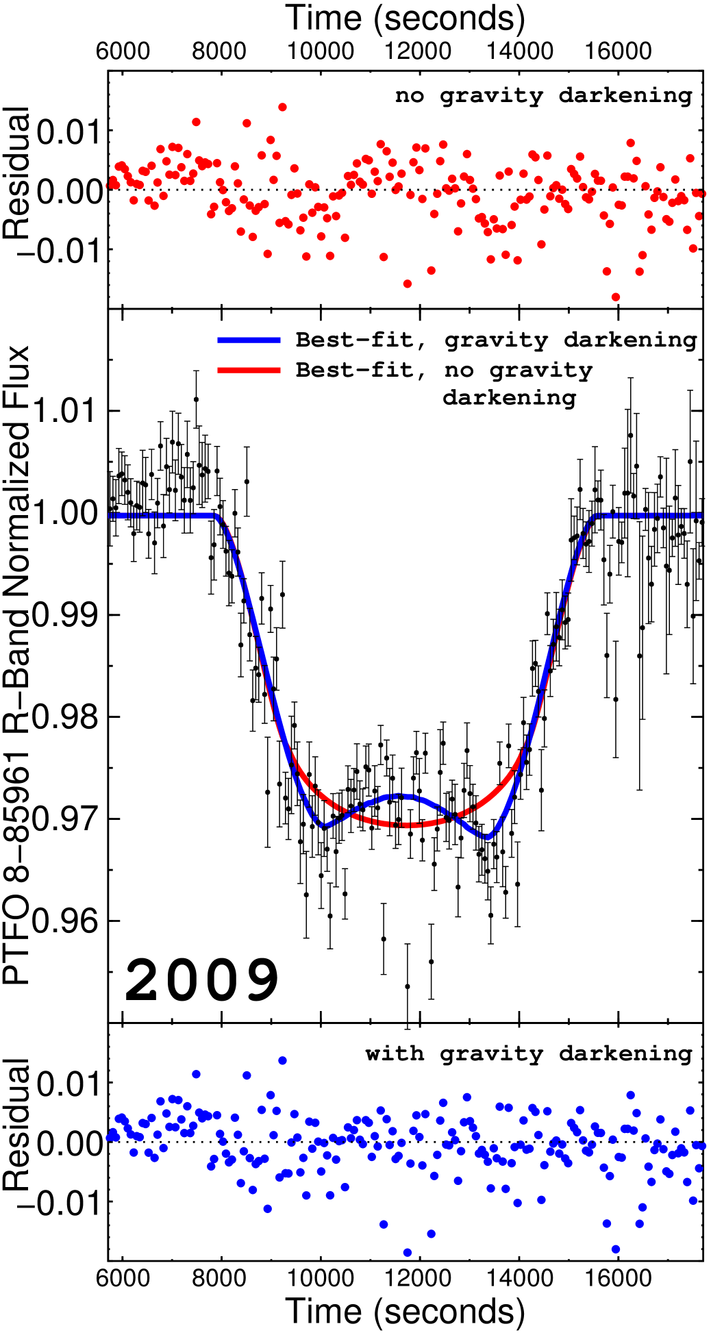
Figure 1.— Photometry and fits for the phase-folded 2009 PTFO 8-8695b lightcurve. We plot the data and fits themselves in the center with the best-fit conventional, no-gravity-darkening model (i.e. with a spherical star) in red and the gravity-darkened model in blue. The residuals from both fits are shown at top (spherical) and bottom (gravity-darkened). The gravity-darkened model does a reasonable job of reproducing the convexity at the bottom of the lightcurve.

Precession of the ascending node of PTFO 8-8695b’s orbit and/or the rotation pole for PTFO 8-8695 could allow gravity darkening to then explain the changes in transit depth and duration changes from 2009 to 2010. Nodal precession has been seen in one other misaligned planetary system so far: KOI-13 (Szabó et al., 2012; Barnes et al., 2011; Szabó et al., 2011a). Gravity darkening has been successfully invoked previously to explain varying shapes of the lightcurves of eclipsing binary stars as well (Philippov & Rafikov, 2013).

In this paper, we investigate whether precession of the planet-star system combined with stellar gravity darkening can explain the unusual lightcurves for PTFO 8-8695b seen by van Eyken et al. (2012) and as we describe in Section 2. We start off by describing the van Eyken et al. (2012) observations in Section 2. In Section 3 we examine the 2009 and 2010 lightcurves separately in the context of gravity darkening. Then in 4 and 5 we develop the theory and a numerical model for orbital precession of Hot Jupiters. We show in Section 6 how that precession would affect the individual fits. And in Section 7, we discuss a self-consistent joint fit that can model the transit observations from both 2009 and 2010 simultaneously. We discuss the implications that the joint fit has on future observations in Section 8 before a discussion and conclusion in Section 9.

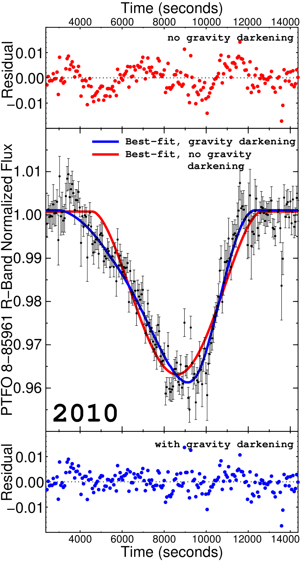
Figure 2.— Photometry and fits for the phase-folded 2010 PTFO 8-8695b lightcurve. We plot the data and fits themselves in the center, with the best-fit conventional, no-gravity-darkening model (i.e. with a spherical star) in red and the gravity-darkened model in blue. The residuals from both fits are shown at top (spherical) and bottom (gravity-darkened). Without gravity darkening the fit is poor. With gravity darkening, the fit is able to tune aggressively to match the transit duration, sharp transit bottom, and long ingress tail simultaneously.

2. OBSERVATIONS

We introduce no new observations in this paper. Instead we reanalyze photometry of PTFO 8-8695 as published in the PTFO 8-8695b discovery paper by van Eyken et al. (2012). As part of the the Palomar Transient Factory Orion (PTFO) campaign, van Eyken et al. (2012) acquired R-band relative photometry of PTFO 8-8695 during all or portions of 11 separate transits of PTFO 8-8695b between 2009 December 3 and 2010 January 14 (which we refer to as the “2009” observations), and 6 separate transits between 2010 December 8 and 2010 December 14.

As a T-Tauri star, PTFO 8-8695 shows significant amounts of stellar variability owing to starspots and activity. These spots manifest as red noise in the resulting lightcurve. The stellar rotational modulation induced by starspots occurs on a much longer timescale than the transit, and thus we remove it using a spline fit to the out-of-transit points. However, variations in the lightcurve that might result from the planet passing over individual starspots or starspot clusters likely remain. Such starspot crossings have been seen for other transiting planets (e.g. Pont et al., 2007), and have in some cases been used to measure spin-orbit alignment via the pattern of starspot crossings on successive transits (e.g. Désert et al., 2011; Nutzman et al., 2011). Because the typical lifetime for sunspots is days to a couple of weeks, any starspot effects on the transit lightcurve shape in the PTFO 8-8695 system should decohere on that timescale.

Therefore to average out any potential starspot crossings, we combine the 11 2009 transits and 6 2010 transits into two lightcurves, one for each season. We fold the lightcurves with the van Eyken et al. (2012) period of 0.44143 days and then combine the observations into 1-minute bins. However, in averaging away the potential influence of stellar activity, we introduce additional error into each photometric measurement. We account for that additional error by increasing the size of our 1-$\sigma$ errors on measured parameters based on the reduced $\chi^{2}$, but that correction may not fully account for stellar activity variability.

We show the resulting photometry for the 2009 transits in Figure 1, and for the 2010 transits in Figure 2. The two lightcurves are distinctly different. Moreover, this difference in shape is evident when comparing individual transits (i.e., not the folded and binned versions) as well (see Figure 6 from van Eyken et al., 2012).

The 2009 transit is both shallower in depth and longer in duration than the 2010 transit. That combination is bizarre. Transits can conceivably change in duration (Transit Duration Variations, or TDVs) over time due to periapsis precession (Pál & Kocsis, 2008), nodal precession (Miralda-Escudé, 2002), or perturbation from moons (Kipping, 2009) and other planets in the system (Nesvorny et al., 2013). In fact, nodal precession from stellar oblateness has already been detected in one system, KOI-13, from TDVs (Szabó et al., 2012).

TDVs would also be expected to associate with changes in transit depth. Shorter duration transits imply a higher transit impact parameter, $b$, with a transit chord closer to the stellar limb. The stellar disk darkens near the limb as a result of limb darkening. Therefore a planet transit that evolves to shorter duration should also have a shallower depth.

But the PTFO 8-8695b lightcurve gets shorter and deeper. That combination implies a planet transiting nearer the stellar limb, but with that limb being brighter than the center of the stellar disk. Limb brightening is seen in planets with strong gaseous absorbers (like reflected light from Titan when viewed at wavelengths where methane absorbs, Young et al., 2002). But limb brightening cannot happen in adiabatic stellar photospheres.

The associated phenomenon of gravity darkening, however, could help to solve the problem. The above discussion of TDVs assumes a stellar rotation slow enough to have a negligible effect on the disk profile — the star can thus be treated as spherical. As showed by von Zeipel (1924), a star that rotates fast enough to become oblate also shows significant variation in brightness across its disk. Near the stellar equator where the local effective gravity is lower as a result of centrifugal acceleration, the atmospheric scale height is commensurately higher. Consequently, the photosphere occurs at a lower pressure level at the equator than it does at the poles, with a correspondingly lower temperature.

The resulting gravity-darkened stellar disk shows hotter and brighter poles along with cooler and dimmer equatorial regions. Interferometric imaging of the stellar disks of nearby rapidly rotating stars has empirically confirmed the gravity darkening concept (e.g., Peterson et al., 2006; Monnier et al., 2007; van Belle, 2012). Gravity darkening also affects the lightcurves of eclipsing binary stars (Philippov & Rafikov, 2013), and has been seen in one other transiting exoplanet lightcurve (KOI-13.01, Szabó et al., 2011b; Barnes et al., 2011).

The PTFO 8-8695b lightcurve could potentially be explained therefore as a planet transiting a gravity-darkened star. In this scenario, the longer, shallower 2009 transits result from a low transit impact parameter as the planet traverses across the stellar equator. The shorter, deeper transits from 2010 would then represent more nearly grazing transits that cross near the bright stellar pole.

In order for the gravity-darkening scenario to be plausible, PTFO 8-8695 must be rotating sufficiently rapidly to show significant oblateness. Late-type stars with convective exteriors lose angular momentum over time via stellar winds (this can be used to infer stellar ages, i.e., Meibom et al., 2011). But a very-young star like PTFO 8-8695 would normally be expected to be in the midst of newborn vigorous and rapid rotation.

Present evidence suggests that PTFO 8-8695 does rotate rapidly. A peak in the periodogram of the van Eyken et al. (2012) photometry with a period near that of the planetary orbit implies synchronous rotation with a period of 10.76 hours. Spectroscopy shows rotational broadening of the stellar lines amounting to $v\sin i=80.\pm 8~{}\mathrm{km/s}$, broadly consistent with synchronous rotation given the stellar radius.

The star’s youth further factors in the favor of gravity darkening because of its large radius. Still undergoing gravitational contraction along the Hayashi track (Hayashi, 1961), the star’s radius is large ($1.07~{}\mathrm{R_{\odot}}$, van Eyken et al., 2012) given its low mass ($0.34~{}\mathrm{M_{\odot}}$ or $0.44~{}\mathrm{M_{\odot}}$ depending on the model, Briceño et al., 2005). The big radius increases the centrifugal acceleration at the equator, which is proportional to $R_{*}$ for a given rotation period. The large radius also means that the surface gravity is lower than it would be for an M-dwarf on the main sequence.

That lower gravity leads to greater gravity darkening differences between the equator and pole because the local emitted photospheric flux is proportional to $g_{\mathrm{eff}}=g-a_{\mathrm{centrifugal}}$. The equator-to-pole flux ratio is therefore equal to

$$\frac{F_{\mathrm{equator}}}{F_{\mathrm{pole}}}=\frac{g_{\mathrm{eq}}}{g_{\mathrm{p}}}=\frac{g-a_{\mathrm{centrifugal}}}{g}=\frac{g-R_{*}\omega^{2}}{g}$$ (1)

for a stellar angular rotation rate of $\omega$. With low gravity $g$, a large stellar radius $R_{*}$, and rapid rotation $\omega$, PTFO 8-8695 would seem an excellent candidate for gravity darkening.

Plugging in conservative values from van Eyken et al. (2012) for these quantities ($R_{*}=1.07~{}\mathrm{R_{\odot}}$, $g=105~{}\mathrm{m/s^{2}}$, $\omega=2\pi/10.76$ hrs) yields to equator-to-pole flux ratios around $0.8$. The poles would then be 25% brighter than the equator. PTFO 8-8695’s oblateness would be $f\sim 0.1$. Not only could PTFO 8-8695 be gravity darkened, if the measurements are even close to right, it must be gravity darkened.

3. INDIVIDUAL FITS

To evaluate whether gravity darkening on PTFO 8-8695 could plausibly be responsible for the unusual PTFO 8-8695b transit lightcurves, we first fit the 2009 December and 2010 December lightcurves separately. To fit the PTFO 8-8695b transit lightcurve, we use the program transitfitter, as developed in Barnes (2009) and Barnes et al. (2011). It uses a Levenberg-Marquardt $\chi^{2}$ minimization routine to drive a numerical lightcurve model. The numerical model computes an explicit two-dimensional integral across the portion of the stellar disk occulted by the planet (see Section 5 below for more details about the transitfitter algorithm).

In order to serve as a robust test for gravity darkening, we conservatively assume a worst-case stellar mass of $M_{*}=0.44~{}\mathrm{M_{\odot}}$ for PTFO 8-8695. We adopt a planet-synchronous stellar rotation period of 0.44841 days (van Eyken et al., 2012). We assume a combined quadratic limb-darkening parameter (after Brown et al., 2001) of $c_{1}=u_{1}+u_{2}=0.735$, as determined from theoretical calculations by Claret et al. (1995). To simulate the R-band photometric observations, we model a monochromatic transit at 0.658 $\mu\mathrm{m}$. We also assume that the planet’s orbit is circular.

In fitting individual lightcurves, we hold limb darkening coefficient $c_{1}$, the orbital period $P$, and $M_{*}$ constant. We dynamically fit for $R_{*}$, the planet radius $R_{p}$, the time at inferior conjunction $t_{0}$, and the out-of-transit stellar flux $F_{0}$. Spin-orbit alignment is a function of the planetary orbit inclination $i$, the projected alignment $\lambda$, and the stellar obliquity to the plane of the sky $\psi$. Figure 3 shows a diagram of these three alignment variables. We fit for all three of them in the case of the gravity-darkened star, but just for $i$ in the case of no limb darkening (when changing $\lambda$ and $\psi$ has no effect on the lightcurve).

We fit each lightcurve with both a gravity-darkened rotating star model (blue in figures) and a conventional non-rotating spherical star model with no gravity darkening (red in figures). Table 1 contains the resulting best-fit system parameters, based on angle definitions as shown in Figure 3. Figures 1 and 2 show the observations, best-fit spherical and gravity-darkened lightcurves (both from transitfitter), and fit residuals.

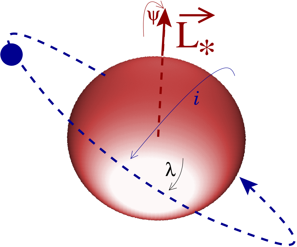
Figure 3.— Definitions of our angular geometric quantities. The planet’s orbital inclination is $i$, measured toward the observer from the plane of the sky. The planet’s projected spin-orbit angle is $\lambda$, as measured clockwise from stellar east. The stellar obliquity to the plane of the sky, $\psi$, is measured as the angle that the north stellar pole is tipped away from the plane of the sky.

	$\chi^{2}_{r}$	$R_{*}$ ($\mathrm{R_{\odot}}$)	$R_{p}$ ($\mathrm{R_{Jup}}$)	$t_{0}$ (s)	$i$	$\lambda$	$\psi$
2009 only, no gravity darkening	2.43	$1.00\pm 0.06$	$1.60\pm 0.14$	$30861720\pm 50$	$74^{\circ}\pm 5^{\circ}$	—	—
2009 only, with gravity darkening	2.11	$1.19\pm 0.07$	$2.00\pm 0.17$	$30861700\pm 200$	$64^{\circ}\pm 3^{\circ}$	$90.^{\circ}\pm 22^{\circ}$	$2^{\circ}\pm 19^{\circ}$
2010 only, no gravity darkening	2.24	$0.98\pm 0.14$	$5.4\pm 2.1$	$60848600\pm 50$	$45^{\circ}\pm 7^{\circ}$	—	—
2010 only, with gravity darkening	1.54	$1.39\pm 0.11$	$1.80\pm 0.20$	$60848300\pm 290$	$58^{\circ}\pm 5^{\circ}$	$136^{\circ}\pm 33^{\circ}$	$31^{\circ}\pm 25^{\circ}$
2009 & 2010, no gravity darkening	3.03	$1.15\pm 0.04$	$2.11\pm 0.14$	$60848560\pm 70$	$61^{\circ}\pm 2^{\circ}$	—	—

Table 1Best-fit values for fits of the 2009 and 2010 PTFO 8-8695b transit lightcurves, with and without gravity darkening. Angles $i$, $\lambda$, and $\psi$ are as shown in Figure 3. The epoch time $t_{0}$ is measured in seconds past 2009 January 1 at midnight UTC.

3.1. 2009 Transit

In 2009 (Figure 1), the transit bottom is flat — or possibly even convex. A conventional spherical star fit (i.e., one without gravity darkening, shown in red) cannot reproduce this convexity at all. The gravity-darkened star fit (in blue) does a reasonable job of reflecting the transit bottom convexity by having the planet transit chord perpendicular to the stellar equator. We measure that angle as the projected spin-orbit alignment angle $\lambda$ where $\lambda$ is measured clockwise from stellar east. The star itself has a low obliquity to the plane of the sky, $\psi$ (where $\psi=i-90^{\circ}$ with $i$ being the conventional stellar inclination relative to the line of sight).

We show a graphical representation of the transit geometry in the left subfigure in Figure 4. By transiting perpendicular to the oblate stellar equator, the total transit duration is shorter than the equivalent $\lambda=0$ transit by a factor of $1-f$ where $f$ is the stellar oblateness.

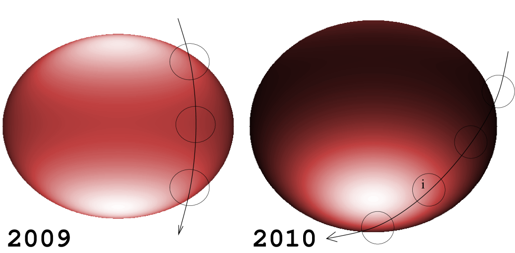
Figure 4.— Transit geometry of the best-fit gravity-darkened models for 2009 (left) and 2010 (right) photometry of PTFO 8-8695. The two images are to scale, accounting for different best-fit stellar radii in the two cases (see Table 1). The larger best-fit radius in 2010 leads to more severe gravity darkening at the stellar equator. In each image the planet’s projected path is shown as a series of appropriately scaled black circles separated in time by 2400 seconds (40 minutes). The apparent curvature of the projected paths is real: it derives from tracking of the full three-dimensional planetary orbit trajectory in this unusual case where the planet’s orbit is less than 2 stellar radii in semimajor axis. The center planet circle from 2009 corresponds to inferior conjunction. In 2010 the circle with the tiny mark in it (an ‘i’) denotes inferior conjunction — an oblique transit path across a gravity-darkened, oblate star leads to the long transit duration and asymmetric lightcurve evident in the photometric data (Figure 2).

The planet first transits the oblate star at relatively high stellar latitude. Nearer the pole the stellar photosphere is hotter, and therefore the stellar flux is higher. This effect is compensated by the countervailing effect of limb darkening, however, leading to total planet-occulted fluxes that are not too different from those at mid-transit when the planet covers the cooler (and dimmer) equator.

If anything, the gravity-darkened model underfits the intensity of the ‘horns’ on the lightcurve that lead to the transit bottom convexity. We could exaggerate the horns in the fit by increasing the gravity darkening parameter $\beta$ (von Zeipel, 1924), which we fix at $\beta=0.25$. However based on the overall accuracy of the data, the error for which is significantly increased by stellar spots and flares, we elect not to modify $\beta$ at this time to avoid overfitting. Additional observations can reduce the overall noise level and may permit a measurement of $\beta$ in the future.

The lightcurve is nearly symmetric for this $\lambda=90^{\circ}$ transit, with the small best-fit asymmetry provided by the slight stellar obliquity in this fit (north pole pointed $2^{\circ}$ away from the observer). The relatively high errors for the spin-orbit angles $\lambda$ and $\psi$ result from the model’s ability to fit the flat transit bottom near-equally well by decreasing (increasing) the projected angle $\lambda$ and increasing (decreasing) the stellar obliquity $\psi$. That degeneracy also leads to greater uncertainty in the time of inferior conjunction $T_{0}$. With an oblate star, transits with projected alignments $\lambda$ that differ from $0^{\circ}$, $90^{\circ}$, $180^{\circ}$, and $270^{\circ}$ have mid-transit times that do not coincide with the time of inferior conjunction, as might usually be assumed.

Note the arced projected planet trajectory in Figure 4. It is real. Because the planet’s semimajor axis is so tiny — less than 2 stellar radii – approximating the planet’s path as straight no longer provides sufficient fidelity.

3.2. 2010 Transit

The 2010 lightcurve (Figure 2) has a significantly different shape to that from 2009. Instead of a flat transit bottom, the transit bottom is sharply peaked. It shows no convexity. And it is decidedly asymmetric, with a long tail toward the ingress side.

The spherical-star (non-gravity-darkened) model does a particularly poor job of fitting the 2010 transit. Specifically, our model is unable to reproduce the long ingress tail. In fitting for the high transit bottom curvature (the ‘V’ shape) without gravity darkening, the model runs off the rails toward a grazing transit for an unreasonably large planet radius ($R_{\mathrm{p}}=5.4\pm 2.1~{}\mathrm{R_{Jup}}$).

On the other hand, the gravity-darkened fit reproduces the 2010 lightcurve well. We show the best-fit gravity-darkening transit geometry at right in Figure 4.

The precise shape of the ingress tail drives the fit toward a higher stellar radius than the 2009 fit: $1.39~{}\mathrm{R_{\odot}}$ (2010) as opposed to $1.19~{}\mathrm{R_{\odot}}$ (2009). The $1.39~{}\mathrm{R_{\odot}}$ matches precisely the spectroscopically-derived value from Briceño et al. (2005). However, given that the analysis of the spectroscopy did not account for the gravity-darkened nonuniformity of emission across the stellar disk, the similarity in stellar radius values is likely coincidence. Slight changes to the tail shape, as might be present but swamped by stellar noise, could allow for smaller stellar radii.

The larger inferred stellar radius ($1.39~{}\mathrm{R_{\odot}}$ vs. $1.19~{}\mathrm{R_{\odot}}$) observed in 2010 than in 2009 drives more severe gravity darkening at the stellar equator. The fit’s sharp transit bottom derives from a transit path that crosses near the hot but small stellar polar region. The long total transit duration results from a transit that starts at the stellar equator and maximizes its interior path using the inherent orbital curvature. The long tail then arises due to an early ingress along the cold and dim stellar equator.

The radius discrepancy may owe to the inherent noisiness of the lightcurve as driven by stellar activity. In particular the 2010 tail at ingress could be an artifact resulting from an imperfect fit to the out-of-transit stellar variation. In order to resolve the radius discrepancy, we need to simultaneously fit both lightcurves so as to force the fit into coherence. Such a simultaneous fit requires an understanding of how the transit geometry could evolve from that seen in 2009 to that seen in 2010. Precession of the stellar spin and planetary orbit angular momenta could provide such a mechanism.

4. PRECESSION

The gravity-darkened best-fit values for the 2009 and 2010 transits show reasonable agreement, given that they were fit separately. The stellar and planetary radii overlap within $2\sigma$. The spin-orbit parameters $\lambda$ and $\psi$, however, are very different. Taking into account the highly oblate star and tiny planetary orbit semimajor axis (just $1.7~{}\mathrm{R_{*}}$), though, the two measurements could be reconciled if the planet-star system experienced precession in the intervening year.

4.1. Form of Precession

In the case of a two-body system consisting of an oblate star and a close-in planet, torques between the planet and the star’s rotational bulge induce nodal precession (Figure 5). Similar precession scenarios are familiar within the solar system, where the Earth’s spin and orbit both precess.

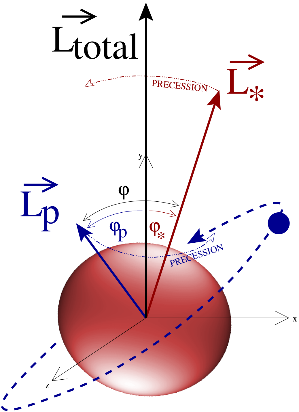
Figure 5.— Precession geometry for the case of an oblate star (red) orbited by a single planet (blue). Both the stellar spin angular momentum ${\vec{L}_{*}}$ and the planetary orbit angular momentum ${\vec{L}_{p}}$ precess around the system’s invariable plane, defined by ${\vec{L}_{\mathrm{total}}}$. In the case where $L_{*}\gg L_{p}$ the geometry reduces to ${\vec{L}_{p}}$ precessing around ${\vec{L}_{*}}$, as for the International Space Station precessing around Earth, for example. When $L_{p}\gg L_{*}$, then ${\vec{L}_{*}}$ effectively precesses around ${\vec{L}_{p}}$, as would happen in a Sun-Jupiter system in the absence of other bodies. In the case of PTFO 8-8695b, ${\vec{L}_{p}}\sim{\vec{L}_{*}}$, and the more complex geometry described in this figure is required, where ${\vec{L}_{p}}$ and ${\vec{L}_{*}}$ both precess around the net angular momentum of the system ${\vec{L}_{\mathrm{total}}}$. The precession arrows show the direction of ‘positive’ precession in the mathematics. In reality the precession is negative, i.e. retrograde, or clockwise as seen from above the stellar north pole.

Earth’s rotation axis precesses around the plane containing the Sun every 26,000 years, resulting from torques applied to its rotational bulge by the Sun and the Moon. This process maintains Earth’s obliquity (axis tilt), changing only the azimuthal direction in which the axis points.

Earth’s orbit is inclined by $1.57^{\circ}$ with respect to the solar system’s invariable plane — the plane normal to the solar system’s net angular momentum vector ${\vec{L}_{\mathrm{total}}}$. Earth’s orbital angular momentum vector ${\vec{L}_{p}}$ precesses around ${\vec{L}_{\mathrm{total}}}$ every $\sim 100,000$ years. Jupiter’s gravity provides the dominant torque driving the precession of Earth’s orbit, though, not the Sun’s rotational bulge.

The case of PTFO 8-8695b is more complex than that of the Earth’s precessions owing to the similarity of the magnitudes of the stellar spin angular momentum $|{\vec{L}_{*}}|\equiv L_{*}=\mathbb{C}M_{*}R_{*}^{2}\omega$ and the planetary orbit angular momentum $|{\vec{L}_{p}}|\equiv L_{p}=M_{p}a_{p}^{2}n$, where $\mathbb{C}$ is the moment of inertial coefficient (0.4 for a uniform-density sphere, 0.059 for the Sun), $M_{*}$ is the stellar mass, $R_{*}$ is the stellar radius, $\omega$ is the stellar rotation rate (in, say, radians per second), $M_{p}$ is the planetary mass, $a_{p}$ is the planetary orbital semimajor axis, and $n$ is the planet’s orbital mean motion (again in radians per second). We assume a circular orbit here for simplicity. Szabó et al. (2012) investigated a similar case where $L_{p}\sim L_{*}$ in the case of exoplanet KOI-13.01. The ratio of the system angular momentum represented by the planet’s orbit to that in the stellar spin is

$$\frac{L_{p}}{L_{*}}=\frac{1}{\mathbb{C}}\frac{M_{p}}{M_{*}}\frac{n}{\omega}\bigg{(}\frac{a}{R_{*}}\bigg{)}^{2}~{}~{}~{}~{}.$$ (2)

Using parameters from Briceño et al. (2005) and van Eyken et al. (2012), as shown in our Table 2, the possible values of $\frac{L_{p}}{L_{*}}$ for the PTFO 8-8695b system range from 0.080 if $M_{p}=1.0~{}\mathrm{M_{Jup}}$ to 0.45 if $M_{p}=5.5~{}\mathrm{M_{Jup}}$ (the van Eyken et al. (2012) radial velocity upper limit).

$M_{*}$	$0.34~{}\mathrm{M_{\odot}}$ or $0.44~{}\mathrm{M_{\odot}}$
$R_{*}$	$1.39~{}\mathrm{R_{\odot}}$
$\mathbb{C}$	0.059
$\omega=n$	$0.44841\pm 0.00004$ days
$a_{p}$	$1.80~{}\mathrm{R_{\odot}}$
$M_{p}$	$\leq 5.5\pm 1.4~{}\mathrm{M_{Jup}}$

Table 2PTF-1 system parameters, from Briceño et al. (2005) and van Eyken et al. (2012).The value for the stellar moment of inertia coefficient $\mathbb{C}$ is assumed to be that of the Sun.

Hence, in the case of PTFO 8-8695b, the stellar spin pole and the planetary orbit normal both precess around their mutual net angular momentum vector as shown in Figure 5. To quantify the geometry, we define $\varphi$ to be the angle between ${\vec{L}_{*}}$ and ${\vec{L}_{p}}$. This value, the spin-orbit angle, is constant as a function of time (assuming that there are no other objects in the system that affect it on the same timescale). We then separately define individual obliquities $\varphi_{p}$ and $\varphi_{*}$ to be the angular distances between ${\vec{L}_{p}}$ and ${\vec{L}_{\mathrm{total}}}$, and between ${\vec{L}_{*}}$ and ${\vec{L}_{\mathrm{total}}}$ respectively. The two sum to $\varphi$,

$$\varphi_{p}+\varphi_{*}=\varphi~{}~{},$$ (3)

with

$$\frac{\sin{\varphi_{p}}}{\sin{\varphi_{*}}}=\frac{L_{*}}{L_{p}}~{}~{}~{}.$$ (4)

The mutual precession of ${\vec{L}_{p}}$ and ${\vec{L}_{*}}$ is driven by the torque $\vec{\tau}$ between the planet and the stellar rotational bulge. The rates of change of the angular momentum vectors $\frac{d{\vec{L}_{p}}}{dt}$ and $\frac{d{\vec{L}_{*}}}{dt}$ are equal and opposite according to Newton’s third law:

$$\vec{\tau}\equiv\frac{d{\vec{L}_{p}}}{dt}=-\frac{d{\vec{L}_{*}}}{dt}~{}~{}~{}.$$ (5)

The magnitude of the torque in the case where $L_{p}\sim L_{*}$ is identical to that in the endpoint cases when $L_{p}\gg L_{*}$ or $L_{p}\ll L_{*}$. But in the $L_{p}\sim L_{*}$ case, instead of ${\vec{L}_{p}}$ precessing around in a circle with a total circumference of $2\pi L_{p}\sin{\varphi}$ (as it does when $L_{p}\ll L_{*}$), it must instead traverse a distance of $2\pi L_{p}\sin{\varphi_{p}}$. Therefore given the precession rate $\dot{\Omega}_{p}$ for the longitude of the ascending node of the planet’s orbit in the simpler $L_{p}\ll L_{*}$ case, then the full mutual precession rate $\dot{\Omega}$ for the $L_{p}\sim L_{*}$ is

$$\dot{\Omega}=\dot{\Omega}_{p}\frac{\sin{\varphi}}{\sin{\varphi_{p}}}~{}~{}~{}.$$ (6)

The precession rate for the stellar rotation pole must be the same, i.e.

$$\frac{\dot{\Omega}_{*}}{\sin{\varphi_{*}}}=\frac{\dot{\Omega}_{p}}{\sin{\varphi_{p}}}$$ (7)

since they precess together, and

$$\dot{\Omega}=\dot{\Omega}_{*}\frac{\sin{\varphi}}{\sin{\varphi_{*}}}~{}~{}.$$ (8)

Equation 6 has some interesting consequences in the $L_{p}\sim L_{*}$ case. First of all, for $\varphi<90^{\circ}$, the full precession rate is always faster than the orbit precession rate from the $L_{p}\ll L_{*}$ case, $\dot{\Omega}>\dot{\Omega}_{p}$. In the limit that $\varphi$ is small, the full precession rate can be approximated as $\dot{\Omega}=\dot{\Omega}_{p}\frac{L_{\mathrm{total}}}{L_{*}}$ — hence a factor of two increase in the equal-angular-momentum case $L_{p}=L_{*}$. However, in a situation where the planet orbits retrograde, $90^{\circ}<\varphi<180^{\circ}$, it is possible to have $\sin{\varphi_{p}}>\sin{\varphi}$, in which case slower, and in some cases extremely slow, precession is possible. For example, take the case where $L_{p}=L_{*}$, and $\varphi=176^{\circ}$. Here the torque is low, but $\varphi_{p}$ is $88^{\circ}$ and ${\vec{L}_{p}}$ must precess all the way around. The result of this thought experiment would be a precession rate 14 times slower than in the $L_{p}\ll L_{*}$ case, all else being equal.

For the expected values for $\frac{L_{p}}{L_{*}}$, full precession rates for PTFO 8-8695b should be between 10% and 50% faster than they would be if we had assumed $L_{p}\ll L_{*}$. Therefore, detection of precession could constrain the planet’s mass both by the precession rate and by the relative amplitude of the stellar and orbital precessions.

4.2. Rate of Precession

The precession rate in systems with $L_{p}\sim L_{*}$ can be calculated using either Equation 6 or Equation 8. Both equations, however, derive from the separate precession rates that are valid for systems with asymmetric angular momentum. In theory, those rates ($\dot{\Omega}_{p}$ and $\dot{\Omega}_{*}$) can be calculated exactly given the stellar mass $M_{*}$, the planetary mass $M_{p}$, the planet’s orbital mean motion $n\equiv 2\pi/P$ (where $P$ is the orbital period), and knowledge of the stellar interior structure.

In a more conventional system where $L_{*}\gg L_{p}$, as for the precession of one of Saturn’s moons for instance, an approximation of the precession rate can be written as (Murray & Dermott, 2000)

$$\dot{\Omega}_{p}=-n\cos{\varphi}\bigg{[}\frac{3}{2}J_{2}\bigg{(}\frac{R_{*}}{a}\bigg{)}^{2}-\frac{27}{8}J_{2}^{2}\bigg{(}\frac{R_{*}}{a}\bigg{)}^{4}-\frac{15}{4}J_{4}\bigg{(}\frac{R_{*}}{a}\bigg{)}^{4}\bigg{]}~{}~{}~{}$$ (9)

to order 4 in $R_{*}/a$. Here $J_{2}$ is the stellar rotation-driven quadrupole moment and $n$ is the planet’s orbital mean motion. This is typically approximated as

$$\dot{\Omega}_{p}=-n\cos{\varphi}\frac{3}{2}J_{2}\bigg{(}\frac{R_{*}}{a}\bigg{)}^{2}$$ (10)

when $R_{p}/a$ is small. Similarly, the stellar precession rate in the opposite limiting case where $L_{p}\gg L_{*}$ might be given as

$$\dot{\Omega}_{*}=-\frac{3}{2}J_{2}\frac{GM_{p}\cos{\varphi}}{a^{3}n\mathbb{C}}~{}~{}~{}~{}.$$ (11)

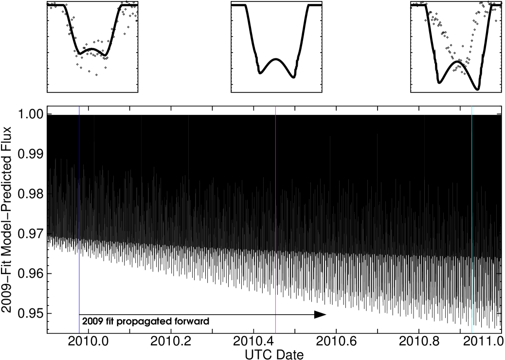
Figure 6.— Forward-extrapolation of the individual fit to the 2009 December photometry. The bottom plot shows the predicted photometric flux seen from PTFO 8-8695 over the course of the year between the 2009 and 2010 observations. This Figure uses as its initial conditions those from the 2009-only fit from Table 1. We show zoom-ins of what individual transits look like inset at top. The colored vertical lines show the times that correspond to the inset transits at top. The best-fit projected alignment value of $\lambda=90^{\circ}$ leads to unusually slow precession for the precise values from Table 1. However other valid sets of transit parameters with $\lambda$ further from $90^{\circ}$ but still within the error bars would see substantially faster precession rates. Note that data points above flux values of 1.002 have been clipped in the insets so that the ranges correspond with the plot at bottom.

A complicating factor is that for PTFO 8-8695b, $R_{*}/a$ is not small at up to 0.77 for $R_{*}=1.39~{}R_{\odot}$ (since $a=1.8~{}\mathrm{R_{\odot}}$). Therefore the higher order terms ($(R_{*}/a)^{4}$ and higher) may substantially contribute. Using the point-core assumption (quite good for stars), the stellar $J_{2}$ is

$$J_{2}=\mathbb{C}f$$ (12)

where $f$ is the stellar oblateness, defined as

$$f\equiv\frac{r_{\mathrm{equatorial}}-r_{\mathrm{pole}}}{r_{\mathrm{equatorial}}}~{}~{}.$$ (13)

Using the PTFO 8-8695 parameters as reported in van Eyken et al. (2012) and shown in Table 2, we calculate that $f=0.20$. Then, incorporating an assumption that the stellar moment of inertia coefficient is $\mathbb{C}=0.059$ (similar to that of the Sun), we calculate that $J_{2}=0.012$ using Equation 12. For spin-orbit angles $\varphi$ near alignment ($\varphi$ small), the first term in Equation 9 is $\dot{\Omega}_{p}=1.6\times 10^{-6}$ radians/s, corresponding to a precession period of just 45 days! This value is consistent with a different calculation by van Eyken et al. (2012) that yielded a period of “tens to hundreds of days”.

The second-leading term in Equation 9 yields just $2.6\times 10^{-8}$ radians/s. Therefore despite $R_{*}/a$ not being small, the low $J_{2}$ driven by central mass concentration in the star ($\mathbb{C}=0.059$) allows us to treat the precession rate as in Equation 10 to within a few percent. We therefore adopt Equation 10 for the remainder of the present study.

An additional complication can arise from distortions to the stellar gravitational field due to the tidal bulge induced by the planet. A more careful calculation of $\dot{\Omega}_{p}$ could take into account the higher order $J_{n}$ terms with $n\geq 4$, with $J_{n}$ calculated numerically as suggested by Hubbard (2012). The size of this bulge should vary for an inclined planet as the stellar radius changes with sub-planetary latitude. This effect in combination with the non-prolate nature of the tidal bulge due to the planet’s proximity (as for HAT-P-7, Jackson et al., 2012) might necessitate a complete numerical calculation of the average potential around the planet’s orbit in order to most accurately determine $\dot{\Omega}_{p}$.

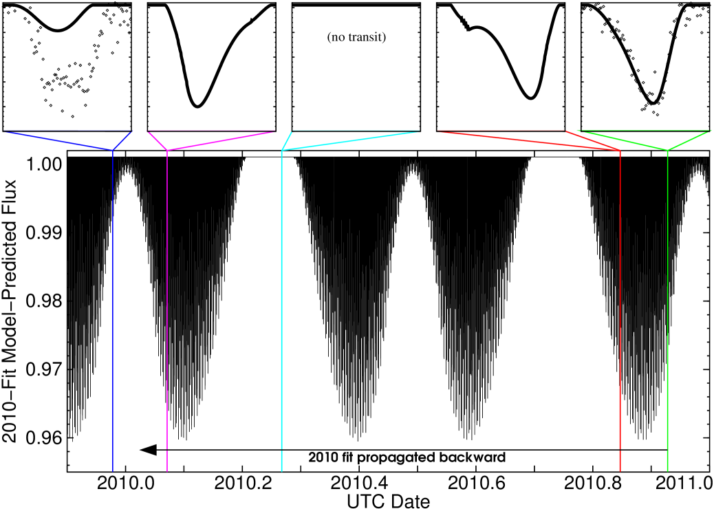
Figure 7.— Backward-extrapolation of the individual fit for the 2010 December photometry. As in Figure 6, the bottom shows a plot of the transit photometry in the time between the 2009 and 2010 observations. The insets at top depict what individual transit events look like at the times shown with colored vertical bars. With a precession period of 179 days, this extrapolation comes close to providing a reasonable explanation for PTFO 8-8695b’s transit lightcurve changes. Particularly interesting is the possibility that the transits may disappear for some portion of the precession cycle.

5. MODEL

The core of the transitfitter lightcurve algorithm is a two-dimensional numerical integration in polar coordinates across the occulted portion of the stellar disk to obtain observed stellar flux. Since that explicit integration is relatively slow (a single fit takes about a day or so to complete), for coarse fits we also use the mostly analytical approximation from Mandel & Agol (2002), Section 5. That approximation does not contain a separate formula for the case when $z\leq p$ (i.e. when the planet covers the point at the center of the stellar disk — we use here the Mandel & Agol (2002) variable definitions that $p\equiv R_{p}/R_{*}$ and $z\equiv d/R_{*}$ where $d$ is the projected separation between the center of the planet and the center of the star). For non-rotating, spherical stars, the usual formula for the stellar flux $I^{*}(z)$ (valid for $z<1-p$) works fine, since the stellar disk is nearly uniform at the geometric center. But for fast-rotating stars, a separate case is needed (parallel to Case 9 in the Mandel & Agol (2002) analytical case):

$$I^{*}(z)=\frac{p^{2}+2pz-z^{2}}{2p^{2}(p+z)^{2}}\int_{0}^{z+p}I(r)2r\mathrm{d}r$$

$$+\frac{(p-z)^{2}}{2p^{2}(p-z)^{2}}\int_{z-p}^{0}I(r)2r\mathrm{d}r~{}~{},$$ (14)

with the radial direction of the integral (the direction matters for gravity-darkened stars since the disk is non-isotropic) being in the direction from the star center toward the planet center. Negative values in the second term indicate an integral in the opposite direction.

The second change that we have made to the algorithm is the incorporation of precession of both the planetary orbit and the stellar spin, as described theoretically in Section 4. The new routine has two parts:

Preprecession:

Whenever there is a change in the projected planetary orbit alignment $\lambda$, the orbital inclination $i$, the stellar obliquity with respect to the plane of the sky $\psi$, the stellar mass $M_{*}$, the planetary mass $M_{p}$, the orbital period $P$, the planetary orbital eccentricity $e$, or the stellar rotation period $P_{\mathrm{rot_{*}}}$, transitfitter calculates time-independent quantities in a process that we call ‘preprecession’. In preprecession, transitfitter executes the following steps:

1. Calculate ${\vec{L}_{p0}}$, the planet orbit angular momentum vector in the sky frame at the time of epoch.

2. Calculate ${\vec{L}_{*0}}$, the stellar spin angular momentum in the sky frame at the time of epoch.

3. Calculate ${\vec{L}_{\mathrm{total0}}}={\vec{L}_{p0}}+{\vec{L}_{*0}}$.

4. Transform ${\vec{L}_{p0}}$ and ${\vec{L}_{*0}}$ into a coordinate system with ${\vec{L}_{\mathrm{total0}}}$ along the $z$-axis as in Figure 5 using Euler angles.

5. Calculate $\dot{\Omega}$ from Equation 6.

Precession:

Then, if either the time $t$ or the epoch $t_{0}$ change, transitfitter calculates the precession using the results of the preprecession calculations:

1. Calculate ${\vec{L}_{p}}(t)$ and ${\vec{L}_{*}}(t)$ in the ${\vec{L}_{\mathrm{total}}}$ frame with a rotation of both through an angle $\dot{\Omega}t$.

2. Transform ${\vec{L}_{p}}(t)$ and ${\vec{L}_{*}}(t)$ back into the sky frame using Euler angles.

3. Update the values for $\lambda$, $i$, $\psi$, and the observationally irrelevant azimuthal angle of the projected stellar spin pole with respect to sky north.

6. EXTRAPOLATION

Using the technical background for precession from Section 4 implemented in transitfitter as described in Section 5, we can now look at whether precession may be responsible for the different PTFO 8-8695 lightcurves seen in 2009 and 2010. To start, we take the best-fit individual solutions from Section 3 and extrapolate forward (2009) and backward (2010) as a test case for the plausibility of the precession hypothesis. For now we assume that $M_{\mathrm{p}}=1.0~{}\mathrm{M_{Jup}}$ with regard to precession rate and $\varphi_{\mathrm{p}}$ calculations.

Figure 6 shows the extrapolation of the 2009 fit. It is clearly not close to being able to explain the 2010 data. The projected alignment $\lambda$ near $90^{\circ}$ is the reason for its failure. Near $\lambda=90^{\circ}$ (and $270^{\circ}$), the planet is in a polar orbit around the star. Hence there is no torque to drive precession forward. The result is a super-long precession period of 8486 days (23 years). Any real value for $\lambda$ would have to be significantly different from $90^{\circ}$ to be consistent with precession. However, because of the high degeneracy between $\lambda$ and $\psi$ for the 2009 fit and the resulting uncertainties in these fitted parameters, such a situation remains plausible.

Extrapolating from the 2010 individual fit yields a much more interesting and plausible result (Figure 7). For the 2010 individual best-fit parameters the precession period is 179 days (in the retrograde direction, and assuming $M_{\mathrm{p}}=1.0~{}\mathrm{M_{Jup}}$). Over the course of those 179 days the transit depth increases, then decreases but does not quite drop to zero before rebounding to the same maximum depth. After the second depth peak, the depth decreases until the transits disappear for about a month. Then the cycle repeats.

The shape of the transits also varies during the precession. During the first half of the cycle the planet transits across the cool stellar equator first, before then crossing at or near the pole. This was the situation for the 2010 December lightcurve. These transits are asymmetric with the deepest part closer to egress. At mid-cycle the transits are shallow and near-symmetric. In the later half of the cycle, the transits are mirror images of those in the first half, transiting the pole first and then the darker low stellar latitudes. Hence in the second half of the cycle the transits are asymmetric with the deepest part on the ingress side.

Note also the shift of mid-transit time for the extrapolated 2009 December data relative to the timing of the actual observed transit. The shift results from the shift in the time of the deepest part of the transit relative to the timing of inferior conjunction (see Figure 4).

Taking the 2009 individual best-fit and extrapolating forward cannot replicate the 2010 transit because of a slow rate of precession that allows for only small changes in $i$, $\psi$, and $\lambda$ in the intervening year. The 2010 individual best-fit cannot reproduce the 2009 data when propagated backwards either, owing to the wrong stellar obliquity $\psi$, planetary inclination $i$, and projected alignment $\lambda$ when evolving the system following the algorithm described in Section 5. The precession-propagated values for the alignment variables $\psi$, $i$, and $\lambda$ are rather sensitive to both the initial values and the planet mass $M_{p}$. Therefore it is possible that using slightly different 2010 initial conditions — equally likely given the uncertainties for those values in Table 1 — along with a different value for $M_{p}$, we could obtain a coherent, self-consistent precession to simultaneously model both lightcurves.

7. JOINT FIT

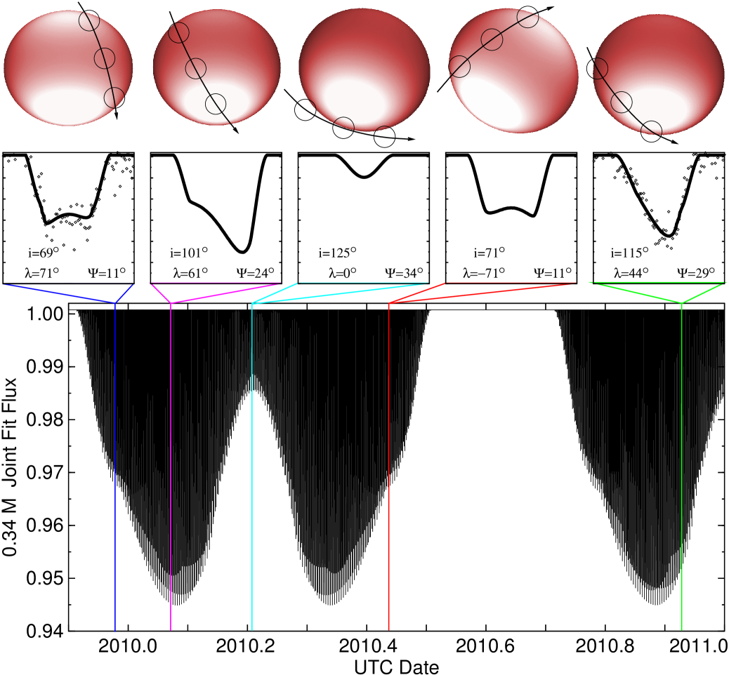
Figure 8.— This figure shows the best-fit self-consistent joint fit to both the 2009 and 2010 photometric data under the assumption that the stellar mass $M_{*}=0.34~{}\mathrm{M_{\odot}}$. The insets at top show the model lightcurves, observed points (open diamonds), and synthetic images with the planet’s trajectory at 5 different epochs between 2009 and 2010. The time of the 2009 observational photometry from van Eyken et al. (2012) is at far left, and the 2010 photometry is the inset at far right. The middle three insets show transit lightcurve shapes and graphic depictions of what the transit might have looked like at three different times between the 2009 and 2010 observations, as predicted by the fit parameters from Table 3. The bottom graph shows the model output over 1.1 years from 2009.9 through 2011.0 UTC, with the times of the insets at top denoted with colored vertical lines. As in the case of the 2010 individual fit shown in Figure 7, this joint fit predicts periods during which the planet does not transit at all during the course of the system’s precession.

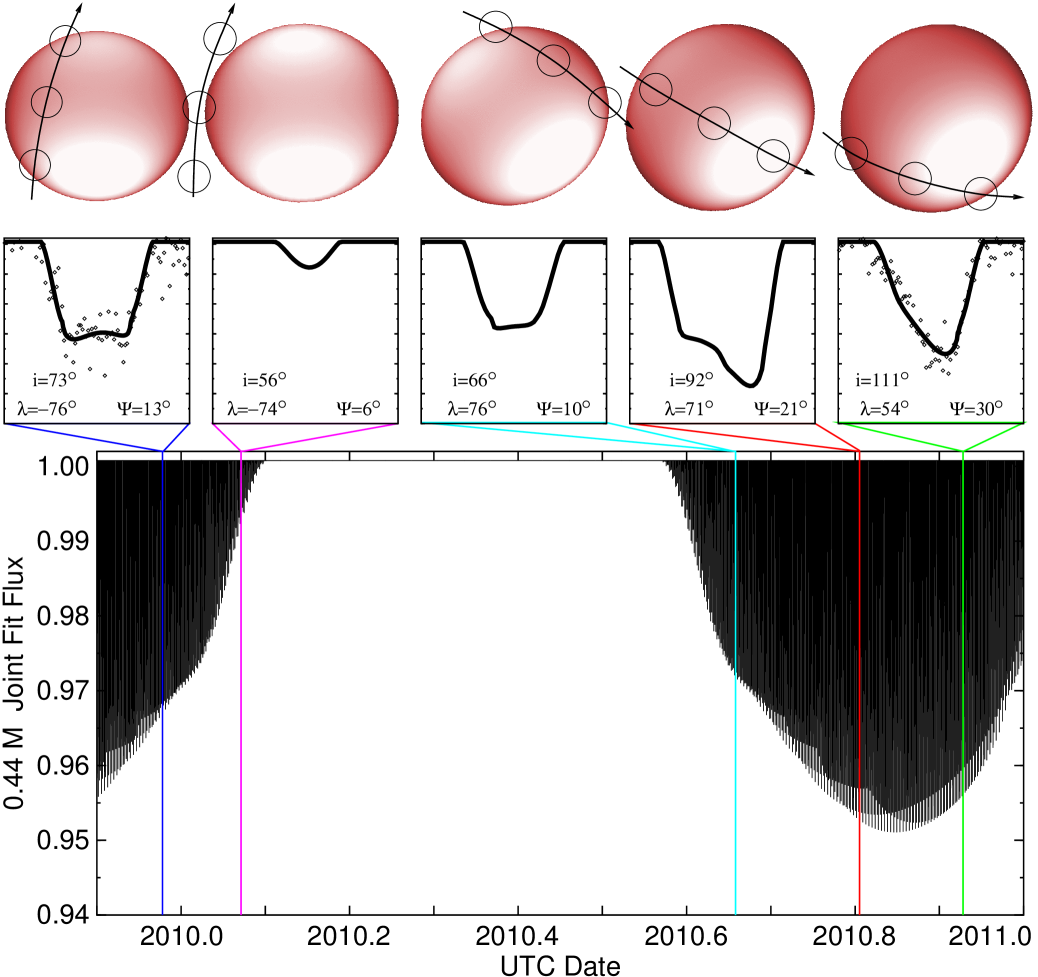
Figure 9.— This figure shows the best-fit self-consistent joint fit to both the 2009 and 2010 photometric data under the assumption that the stellar mass $M_{*}=0.44~{}\mathrm{M_{\odot}}$. The insets at top show the model lightcurves, observed points (open diamonds), and synthetic images with the planet’s trajectory at 5 different epochs between 2009 and 2010. The time of the 2009 observational photometry from van Eyken et al. (2012) is at far left, and the 2010 photometry is the inset at far right. The middle three insets show transit lightcurve shapes and graphic depictions of what the transit might have looked like at three different times between the 2009 and 2010 observations, as predicted by the fit parameters from Table 3. The bottom graph shows the model output over 1.1 years from 2009.9 through 2011.0 UTC, with the times of the insets at top denoted with colored vertical lines. This $M_{*}=0.44~{}\mathrm{M_{\odot}}$ solution precesses more slowly than the $M_{*}=0.34~{}\mathrm{M_{\odot}}$ solution in Figure 8, resulting in less than a full precession cycle between the 2009 and 2010 observational lightcurves.

A complete joint fit of both the 2009 and 2010 observations, accounting for precession and fitting for the planetary orbital period, may be able to comprehensively explain the both the lightcurve shapes and their variability. After an extensive trial-and-error search we were able to identify self-consistent sets of conditions that yield satisfactory simultaneous joint fits to both the 2009 and 2010 lightcurves. The ranges explored included $0.8~{}R_{\odot}<R_{*}<1.6~{}R_{\odot}$, $0<M_{p}<100~{}\mathrm{M_{Jup}}$, and initial (2010) values for $i$, $\psi$, and $\lambda$ within the bounds of the 2010 individual fit and equivalents in both prograde and retrograde directions.

With just two epochs, however, the fits are not necessarily unique. We describe two of them here, one for the assumption of $M_{*}=0.34~{}\mathrm{M_{\odot}}$ and the other for $M_{*}=0.44~{}\mathrm{M_{\odot}}$, each of the spectroscopically-derived stellar masses described in Briceño et al. (2005).

Parameters for Joint Fits
	$0.34~{}\mathrm{M_{\odot}}$	$0.44~{}\mathrm{M_{\odot}}$
$R_{*}$	$1.04\pm 0.01\mathrm{R_{\odot}}$	$1.03\pm 0.01\mathrm{R_{\odot}}$
$R_{p}$	$1.64\pm 0.07\mathrm{R_{Jup}}$	$1.68\pm 0.07\mathrm{R_{Jup}}$
$P$	$0.448410\pm 0.000004$ days	$0.448413\pm 0.000001$ days
$t_{0}$	$60848500\pm 100~{}\mathrm{s}$	$60848363\pm 38~{}\mathrm{s}$
$i$	$114.8^{\circ}\pm 1.6^{\circ}$	$110.7^{\circ}\pm 1.3^{\circ}$
$\lambda$	$43.9^{\circ}\pm 5.2^{\circ}$	$54.5^{\circ}\pm 0.5^{\circ}$
$\psi$	$29.4^{\circ}\pm 0.3^{\circ}$	$30.3^{\circ}\pm 1.3^{\circ}$
$M_{p}$	$3.0\pm 0.2~{}\mathrm{M_{Jup}}$	$3.6\pm 0.3~{}\mathrm{M_{Jup}}$
$\varphi$	$69^{\circ}\pm 3^{\circ}$	$73.1^{\circ}\pm 0.6^{\circ}$
$\varphi_{*}$	$18^{\circ}$	$20.2^{\circ}$
$\varphi_{p}$	$51^{\circ}$	$52.9^{\circ}$
$P_{\dot{\Omega}}$	$-292.6$ days	$-581.2$ days
$f$	0.109	0.083
$\chi_{r}^{2}$	2.17	2.19

Table 3Best-fit parameters from the self-consistent, joint fit of the 2009 and 2010 van Eyken et al. (2012) lightcurves. Epochs $t_{0}$ are measured in seconds after 2009 January 1 00:00 UTC (JD 2454832.5). The orbital period is $P$.

Back-Propagated Alignment Parameters
	$0.34~{}\mathrm{M_{\odot}}$	$0.44~{}\mathrm{M_{\odot}}$
$t_{0}$	30861500 s	30861370 s
$i$	$69.1^{\circ}$	$72.7^{\circ}$
$\lambda$	$71.1^{\circ}$	$-76.1^{\circ}$
$\psi$	$10.7^{\circ}$	$12.8^{\circ}$

Table 4Alignment parameters from the self-consistent, joint fit of the 2009 and 2010 van Eyken et al. (2012) lightcurves as propagated back to the time of the 2009 transit. Our model generates the same lightcurve using these as its initial values as it does using the values at the 2010 epoch shown in Figure 3

Table 3 shows the best-fit parameters for each case: $0.34~{}\mathrm{M_{\odot}}$ and $0.44~{}\mathrm{M_{\odot}}$. In each case, in addition to the fit parameters, which use the mid-transit time of the 2010 observations as their epoch, we show in Table 4 the precessed values as propagated back to the time of the 2009 observations. A graphical representation of the observing geometry as precessed along with transit lightcurves and their evolution in each case are shown in Figures 8 and 9.

We use the covariance matrix from the Levenberg-Marquardt fitting algorithm to generate the quoted errors in Table 3, modified by a correction for the high $\chi^{2}$ of the final fit. The $\chi^{2}$ higher than 1.0 results from accurate photometry of an inherently variable star due to surface activity (starspots). We treat the variability as a source of red noise over and above the photometric precision, compensating for it by multiplying the formal covariance errors by $\sqrt{\chi^{2}}$. This compensation approach is an approximation due to the non-Gaussianity of the stellar variability. A more sophisticated approach like residual permutation (á la Winn et al., 2009) is not warranted given the degeneracy between our two different solutions.

Interestingly, the uncertainties on fit parameters coming out of the joint fit are significantly tighter than the uncertainties from fitting each transit individually. For example, the measured uncertainty on the projected alignment $\lambda$ was $33^{\circ}$ when fitting the 2010 transit individually, and $25^{\circ}$ for the stellar obliquity $\psi$. But when fitting for the 2010 transit along with the 2009 transit and including precession, those uncertanties plummet to $5.2^{\circ}$ and $0.3^{\circ}$ respectively! What’s going on here?

It turns out that the requirement that the 2010 initial conditions propagate backward into the 2009 conditions via precession constrains the system more tightly than do the transit geometries necessary to generate the lightcurve shapes by themselves. With the complex systemic precession as described in Section 4, the initial conditions in 2010 must propagate into the conditions that replicate the 2009 transit. This requirement very tightly constrains the initial values for $\lambda$ and $\psi$, for instance. It also affects the planet mass $M_{p}$ via the partition of the full spin-orbit alignment angle $\varphi$ into $\varphi_{\mathrm{p}}$ and $\varphi_{*}$. If the planet’s mass is too small, then it is unable to pull the star around into the orientation required for the other transit. If the planet’s mass is too big, then it can pull the star around too much. Similarly, in order for the system to arrive in the proper orientation at the right time, the precession period directly constrains the combination of $R_{*}$, $M_{p}$, and $\varphi$.

Essentially these constraints somewhat resemble those for asteroids on a collision course with Earth. Even with uncertain knowledge of an asteroid’s present-day orbital parameters, if you were to know that it was going to collide with the Earth at a certain time in the future, that would by itself give you much more powerful knowledge of what its present-day parameters must be even without better present-day observations. And similar to the asteroid analogy, the further separated in time the target is from the present, the better those constraints will be. Thus future observations of PTFO 8-8695b transits should be capable of driving parameters to such precision that the ultimate uncertainties will be dominated by systematic errors instead of measurement error.

Different precession periods $P_{\dot{\Omega}}$ characterize the two independent solutions.

7.1. Stellar Mass $M_{*}=0.34~{}\mathrm{M_{\odot}}$ Case

In the $M_{*}=0.34~{}\mathrm{M_{\odot}}$ case, the precession period is 292.6 days (in the retrograde direction, hence the negative sign in Table 3). The system therefore undergoes 1.25 precessions in between the 2009 and 2010 van Eyken et al. (2012) lightcurves. The spin-orbit misalignment angle of $\varphi=69^{\circ}$ makes this a highly inclined planet orbit. But with $\varphi=69^{\circ}$ instead of the $\varphi=90^{\circ}$ (as was the case for the 2009-only fit from Section 3), the precession rate $\dot{\Omega}$ is much faster.

We found this solution by trying various acceptable fits to the 2010 lightcurve alone, then looking at the back-propagation to 2009 and trying to get close enough for the Levenberg-Marquardt solver to zero in on a fit. As such the $M_{*}=0.34~{}\mathrm{M_{\odot}}$ joint fit reproduces the 2010 lightcurve with similar geometry to the individual fit from Section 3. Without precession transit lightcurves around gravity-darkened stars leave a four-fold geometric degeneracy (see Barnes et al., 2011, Figure 3). While the specific geometry shown in Figure 4 indicates a retrograde orbit geometry, the joint fit uses the prograde equivalent of the same geometry.

In numerous searches we were not able to find satisfactory fits under any retrograde solution. This does not necessarily mean that such fits do not exist, only that we did not find one. However, given the effort that we employed in searching, retrograde solutions may very well be ruled out.

In this joint solution, the late 2010 planet initially transits a cool and dim near-equatorial region at ingress, and then the hot bright pole near egress to reproduce the lightcurve asymmetry in the 2010 lightcurve. In contrast to the individual fit, however, the joint fit does a relatively poorer job of fitting the long tail present in the data at ingress. A smaller stellar radius in the joint fit explains the difference.

All of our attempts at a joint fit with $R_{*}\sim 1.4\mathrm{R_{\odot}}$, which would have matched both the 2010 individual fit and the spectroscopic estimate, failed. The short duration of the 2009 transit and its sharp ingress and egress prevent a satisfactory solution for larger stars. This is only true under our assumption of a circular orbit for the planet, of course — if the planet’s orbit were eccentric (e.g. Barnes, 2007; Burke, 2008; Ford et al., 2008), then a solution that matches the spectroscopic radius might still be possible. We did not pursue such a solution, but the addition of more photometric epochs from future observations might allow constraints on orbital eccentricity.

The $R_{*}=1.04\mathrm{R_{\odot}}$ stellar radius from the $M_{*}=0.34~{}\mathrm{M_{\odot}}$ joint fit has other consequences, as well. The smaller radius means a smaller $v\cos{\psi}$ (“$v\sin{i}$”), using our assumed synchronous stellar rotation period. It also leads to less gravity darkening and a lower stellar oblateness.

Gravity darkening breaks the azimuthal degeneracy on the stellar disk, which allows us to determine which part of the star the planet crosses in transit. The broken symmetry leads to our measured planetary inclination of $114.8^{\circ}$ — unusual, considering that inclinations have heretofore always been $0^{\circ}\leq i\leq 90^{\circ}$. By convention, this inclination greater than $90^{\circ}$ indicates that the planet is over the star’s southern hemisphere at inferior conjunction.

When precessed backward to the epoch of the 2009 observations, this fit replicates the flatness of the transit bottom by first transiting near the hot bright north pole, but while that pole is tilted away from the observer. As it travels across the stellar disk to the south, it also moves further from the location of the projected stellar axis, leaving it relatively further from the south pole on egress. By being farther from the brighter pole on egress and closer to the less bright pole on ingress, the transit bottom overall is fairly flat.

The planet’s mass $M_{p}$ drives the overall precession rate $\dot{\Omega}$ and thus the relative placement of the 2009 observation within the precession sequence. All else being equal, higher planetary masses drive faster precessions for prograde orbits by reducing $\varphi_{*}$, as per Equation 8. In transitfitter, these small changes in $M_{p}$ squeeze or extend the precession plot at the bottom of Figure 8 like an accordion.

The planet’s mass also affects the partition of the spin-orbit alignment angle $\varphi$ into the the planet precession angle $\varphi_{p}$ and the stellar precession angle $\varphi_{*}$ as described by Equations 3 and 4. Hence, for larger changes in the planet’s mass, again all else being equal, the shape and character of the transits during precession change as $\varphi_{p}$ and $\varphi_{*}$ change.

Our best-fit value for planet mass in the $M_{*}=0.34~{}\mathrm{M_{\odot}}$ case is $M_{p}=3.0~{}\mathrm{M_{Jup}}$. For masses significantly different than $M_{p}=3.0~{}\mathrm{M_{Jup}}$, on the order of $0.0~{}\mathrm{M_{Jup}}$ or $8.0~{}\mathrm{M_{Jup}}$, the transit shapes change such that flat bottoms do not occur at any time during the precession. For smaller changes in $M_{p}$, different values of $M_{p}$ push the flat-bottomed transits to times incompatible with the 2009 observations.

Note, however, that flat-bottomed transits also occur at another point in the precession cycle. At the time of the red line in Figure 8 (the inset second from right), the transit signatures also have flat bottoms in such a way that could match the shape of the 2009 data. Assuming a zero-mass (test particle) planet extends the precession to bring this second flat-bottom location closer to the 2009 observation epoch, but not all the way there. Faster precession could bring another instance of this second flat-bottom location forward from a new cycle. However, doing so requires a planet mass so large that the precession character alters, and the flat-bottomed portion no longer exists.

Although the observations cannot be explained using the second flat-bottomed area under the assumption that $M_{*}=0.34~{}\mathrm{M_{\odot}}$, our second solution using $M_{*}=0.44~{}\mathrm{M_{\odot}}$ does use its equivalent.

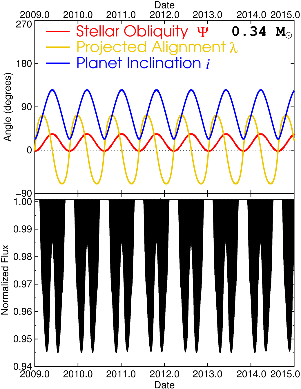
Figure 10.— In this figure we plot the future predicted state of the PTFO 8-8695b system from the $M_{*}=0.34~{}\mathrm{M_{\odot}}$ model. We use black to indicate future transit depth, red to indicate future stellar obliquity to the plane of the sky $\psi$, yellow for future projected spin-orbit alignment $\lambda$, and blue to show future planetary orbital inclination $i$.

7.2. Stellar Mass $M_{*}=0.44~{}\mathrm{M_{\odot}}$ Case

As in the $M_{*}=0.34~{}\mathrm{M_{\odot}}$ case, with $M_{*}=0.44~{}\mathrm{M_{\odot}}$ we were unable to fit both observations using a stellar radius near the spectroscopic value of $1.4~{}\mathrm{R_{\odot}}$. Instead, our best fit in the $M_{*}=0.44~{}\mathrm{M_{\odot}}$ was with a smaller star: $R_{*}=1.03~{}\mathrm{R_{\odot}}$, similar to the best-fit value in the $M_{*}=0.34~{}\mathrm{M_{\odot}}$ case. Thus, the precession period for this $M_{*}=0.44~{}\mathrm{M_{\odot}}$ is longer, owing to a similar radius but higher stellar mass. This leads to higher gravity which results in a less oblate stellar figure (lower $J_{2}$) and therefore lower precession torques and a slower precession rate (see Equations 10 or 11).

The overall geometry for the 2010 epoch is similar to that in the $M_{*}=0.34~{}\mathrm{M_{\odot}}$ fit above (see Figure 9, rightmost inset). The projected alignments $\lambda$ are similar, as are the stellar obliquities. As a result, the total spin orbit alignment $\varphi$ is similar as well. This is essentially the same solution as that for $M_{*}=0.34~{}\mathrm{M_{\odot}}$, except that it uses a conjugate version of the flat-bottomed portion of the precession. Due to the slower precession, this solution reproduces the 2009 data with the opposite projected alignment $\lambda$, resulting in a very similar model lightcurve result.

With slower precession, the $M_{*}=0.44~{}\mathrm{M_{\odot}}$ fit shows a more extended period without transits, in this case fully 6 months long.

The reduced chi squared $\chi_{r}^{2}$ for each fit is similar: 2.17 for $M_{*}=0.34~{}\mathrm{M_{\odot}}$ and 2.19 for $M_{*}=0.44~{}\mathrm{M_{\odot}}$. Both are significantly above 1.0. As a pre-main-sequence M-dwarf, PTFO 8-8695 is particularly noisy, which presumably drives the $\chi_{r}^{2}$ of our fits to be higher than the photon shot noise ideal.

8. FUTURE PROJECTION

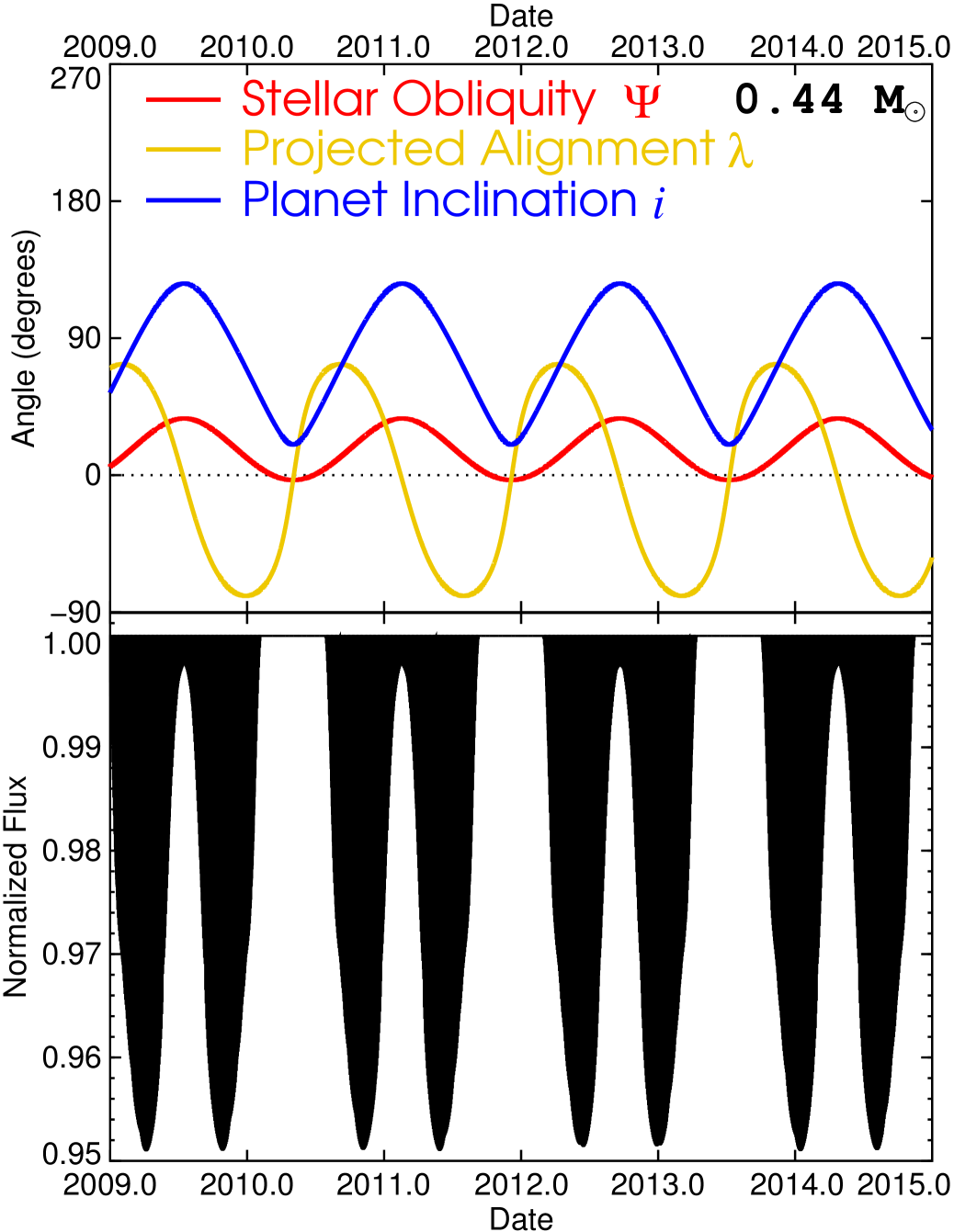
Figure 11.— Same as Figure 10, but for $M_{*}=0.44~{}\mathrm{M_{\odot}}$.

The joint fit offers several avenues for testing the veracity of the precessing gravity-darkened model. Figures 10 and 11 show projections until the end of 2014 for transit depth, planet orbit inclination $i$, the projected spin-orbit alignment $\lambda$, and the stellar obliquity to the plane of the sky $\psi$.

Disappearing Transits

Both joint fit models predict periods of several months during which no transits should occur. At these times, the planet’s impact parameter $b=a\cos(i)/R_{*}$ is greater than $1+\frac{R_{p}}{R_{*}}$, as can be inferred from the planetary orbital inclination, which we plot in blue in Figures 10 and 11. Future photometric campaigns to observe the PTFO 8-8695b transit could confirm our model if they were to show that the transits disappear. Although the times will shift with varying $M_{*}$, the no-transit periods last for 0.21 years with $M_{*}=0.34~{}\mathrm{M_{\odot}}$ and for 0.46 years with $M_{*}=0.44~{}\mathrm{M_{\odot}}$. They recur each cycle, starting at $2010.51+NP_{\dot{\Omega}}$ for $M_{*}=0.34~{}\mathrm{M_{\odot}}$ and $2010.10+NP_{\dot{\Omega}}$ for $M_{*}=0.44~{}\mathrm{M_{\odot}}$ where $N$ is any integer. Non-detections of transits would also place tight constraints on the initial conditions, helping, for instance, to nail down $M_{*}$ or to rule out one of our two $M_{*}$ scenarios.

Changing Orbit Inclination

Related to the disappearance of transits, the predictions for PTFO 8-8695b’s changing orbital inclination could be tested directly by radial velocity (RV) measurements. Sets of RV measurements spanning the planet’s entire orbital phase would be required, each separated in time by several months. The planet’s 10.8-hour orbital period makes it possible to potentially span an orbit in a single night of observing. However, PTFO 8-8695’s large apparent magnitude and high inherent stellar noise would both be problematic for the RV approach.

Changing Stellar Inclination

Our models predict that the star’s rotation pole should be precessing around the net angular momentum vector of the system, as shown in Figure 5. Both fits show that this stellar pole precession should result in changes to the stellar obliquity as measured from the plane of the sky ($\psi$). We show our predictions for changing stellar obliquity as the red curves in Figures 10 and 11. The obliquity should vary between $\sim 0^{\circ}$ and $\sim 30^{\circ}$. Spectroscopy of PTFO 8-8695 over several months’ time could show this changing stellar obliquity using variations in stellar line rotational widths. The line widths should vary as $v\cos(\psi)$ — “$v\sin(i)$” under the conventional definition for $i$ as stellar obliquity to the line of sight. Due to the cosine dependence, however, the variation in $v\cos(\psi)$ should only be $\sim 13\%$.

Changing Stellar Spectrum

As the stellar inclination changes, the star presents to Earth more or less of its hot polar regions. When viewed more nearly pole-on, the star should have a spectrum with a higher effective temperature and an earlier spectral type than when more of the equator is visible. This effect should also lead to long-term changes in the overall magnitude of the star. It should appear brighter when the pole is presented to Earth, and dimmer when the pole is more nearly in the plane of the sky.

Changing Projected Alignment

Nodal precession causes large changes in the projected spin-orbit alignment of the system, $\lambda$, which we show in yellow in Figures 10 and 11. The alignment should vary between $\sim-80^{\circ}$ and $\sim+70^{\circ}$ and should be zero in between during the period of grazing transits (i.e. the second inset from left in Figure 9). These changes in $\lambda$ could be measured from the Rossiter-McLaughlin effect (e.g. Rossiter, 1924; McLaughlin, 1924; Albrecht et al., 2012) or from using stroboscopic starspots (e.g. Désert et al., 2011; Nutzman et al., 2011; Sanchis-Ojeda & Winn, 2011). Practitioners of either method should take care to account for the apparently curved path of the planet across the stellar disk that arises from the very small orbital semimajor axis, as shown in the synthetic images at the top of Figures 8 and 9.

Changing Transit Shapes

A combination of the previous effects leads to changes in the specific transit geometry as a function of time. Those changes manifest as variations in the shape of the planet’s transit lightcurve, seen in the inset lightcurves at the top of Figures 8 and 9. Continued photometric monitoring of the type already done by van Eyken et al. (2012) can confirm the nodal precession of PTFO 8-8695b, differentiate between the two models that we have presented, and allow for precise measurements of all transit parameters, including $M_{*}$.

Chromatic Variation in Transit Shape

Normally, transit lightcurve shapes can show some variability with wavelength due to different degrees of limb darkening. But gravity darkening results from different effective temperatures across the stellar disk. Therefore transit shapes across gravity-darkened stars show significant variation as a function of wavelength (Barnes, 2009). We show predicted transit lightcurves for two additional wavelengths ($0.4~{}\mu\mathrm{m}$ and $2.0~{}\mu\mathrm{m}$, in addition to the R-band $0.638~{}\mu\mathrm{m}$ from the van Eyken et al. (2012) photometry) in Figures 12 and 13. Simultaneous multicolor photometry could confirm the gravity darkening hypothesis and at the same time help to constrain the stellar polar temperature and limb darkening parameters.

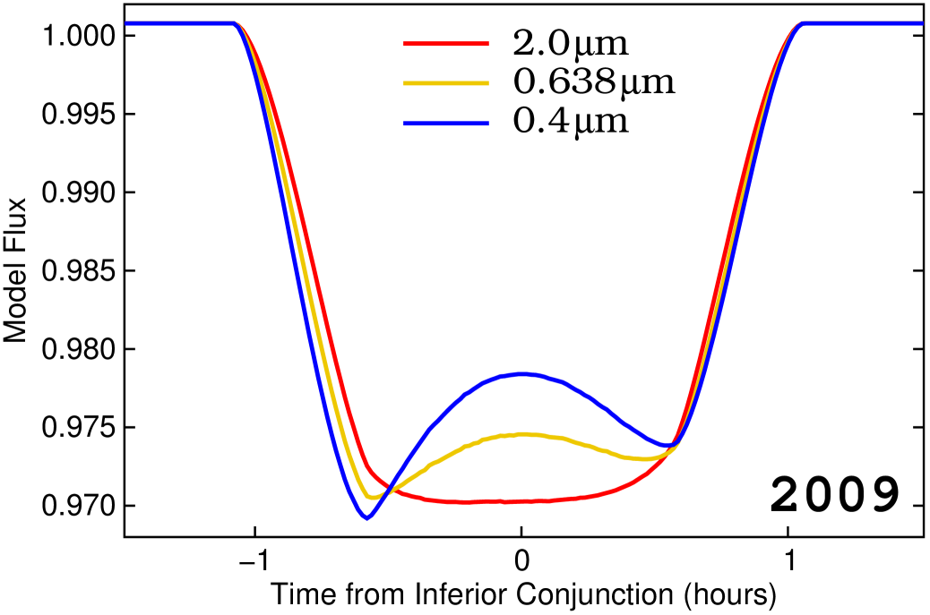
Figure 12.— This figure shows fluxes for the $M_{*}=0.34~{}\mathrm{M_{\odot}}$ model at three different wavelengths: $2.0~{}\mu\mathrm{m}$ (red), $0.638~{}\mu\mathrm{m}$ (yellow), and $0.4~{}\mu\mathrm{m}$ (blue). These three models all assume an identical limb-darkening parameter $c_{1}=0.735$. Usually transits are nearly achromatic, with different fluxes in different wavebands resulting only from different limb darkening. With gravity darkening, however, the transit lightcurve should look substantially different at different wavelengths owing to varying temperatures across the gravity-darkened stellar disk.

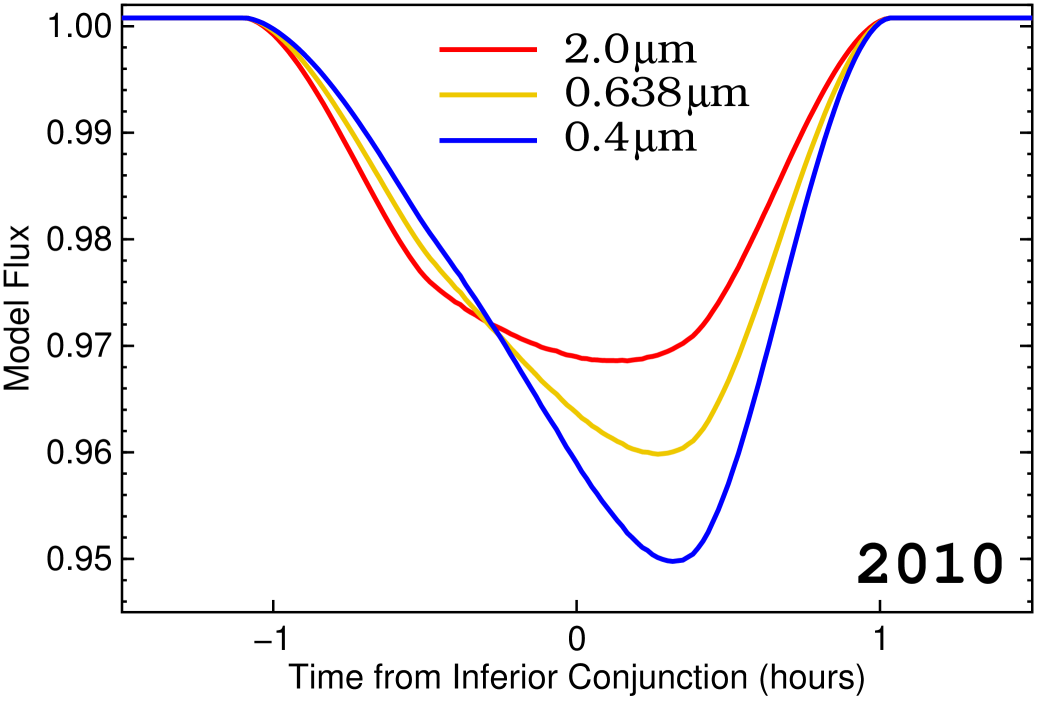
Figure 13.— Same as Figure 12, but for 2010.

9. DISCUSSION AND CONCLUSION

We show that the unusual transit lightcurve shapes of PTFO 8-8695b and their variation can be explained by a precessing planet transiting a gravity-darkened star. If our model is correct, then it would serve as a validation of PTFO 8-8695b as a planet. The van Eyken et al. (2012) discovery paper established an upper limit on the mass of PTFO 8-8695b of $5.5~{}\mathrm{M_{Jup}}$, but could not definitively rule out potential false positives. No false-positive scenario could reproduce the combination of gravity darkening and nodal precession that we see in the PTFO 8-8695 system. We caution, though, that our scenario would need to be verified using the effects from Section 8 to fully confirm PTFO 8-8695b as a planet. PTFO 8-8695b stands to be the second known Hot Jupiter orbiting an M-dwarf star after KOI-254b (Johnson et al., 2012). It would be the only transiting planet known to orbit a T-Tauri star, and that star would be the youngest, coolest, and lowest-mass star to host a transiting planet.

Our measured planetary radii, $1.64~{}\mathrm{R_{Jup}}$ and $1.68~{}\mathrm{R_{Jup}}$, are smaller than that estimated by van Eyken et al. (2012) ($1.91~{}\mathrm{R_{Jup}}$). This difference owes partially to our slightly smaller estimated stellar radius (1.03 or 1.04 $\mathrm{R_{\odot}}$ as opposed to $1.07~{}\mathrm{R_{\odot}}$), and partially to the presumed higher fidelity of our gravity-darkened fit.

Our best-fit masses of $3.0~{}\mathrm{M_{Jup}}$ and $3.6~{}\mathrm{M_{Jup}}$ are consistent with the van Eyken et al. (2012) radial-velocity-derived upper limit of $5.5~{}\mathrm{M_{Jup}}$. Interestingly, these masses and radii place PTFO 8-8695b near to a Roche-lobe-limited state, just barely able to hold on to its atmosphere against tidal disruption (as do the original values from van Eyken et al. (2012), despite the different masses and radii).

The determination of both mass and radius for the planet allows us to place constraints on its composition and thermal evolution. At $3.0~{}\mathrm{M_{Jup}}$ and with $R_{p}=1.64~{}\mathrm{R_{Jup}}$, PTFO 8-8695b is clearly a hydrogen-dominated gas giant, as it lies above the pure hydrogen curve from Fortney et al. (2007). Furthermore, as a brand-new planet PTFO 8-8695b falls very close to the predicted radius curve for a 10-Myr-old $10~{}\mathrm{M_{\oplus}}$-core planet according to tables from Fortney et al. (2007). In particular, the high radius of PTFO 8-8695b at such a young age rules out the “cold start” model for compact initial conditions outlined by Marley et al. (2007).

Our fits show a large misalignment between the stellar spin and the planet orbit of $69^{\circ}$. Such a large misalignment may be inconsistent with the assumption of synchronous stellar rotation. Van Eyken et al. (2012) showed a strong peak in a photometric periodogram corresponding to the planet’s orbital period of 0.448413 days. Van Eyken et al. (2012) interpreted that peak to represent the rotation period of the star, evident in the photometry due to starspots. Synchronous rotation predicts a stellar $v\sin i$ of 102 km/s with our $M_{*}=0.34~{}\mathrm{M_{\odot}}$ best-fit values (similar to the spectroscopically measured value of $80\pm 8~{}\mathrm{km/s}$ from van Eyken et al. (2012)). Thus PTFO 8-8695 is a fast-rotator. However, truly synchronous rotation might be difficult if not impossible to achieve via tidal torques with $\varphi=69^{\circ}$. Future photometry of transit shapes for PTFO 8-8695b may allow for a dynamical fit for stellar rotation rate, which should help to shed light on the accuracy of the synchronous stellar rotation determination.

The high spin-orbit misalignment of $\varphi=69^{\circ}$ has implications for planet formation and evolution. PTFO 8-8695b is not the only near-polar-orbiting Hot Jupiter (e.g., Kepler-63b, Sanchis-Ojeda et al., 2013). But the presence of such a highly inclined planet around such a young star supports the idea from Winn et al. (2010) that Hot Jupiters either form with random orientations or very quickly acquire random orientations after their formation. Furthermore, the young age of this highly inclined planet indicates that PTFO 8-8695b could not have formed by Kozai resonance followed by tidal evolution, as some Hot Jupiters may have (Wu & Murray, 2003; Fabrycky & Tremaine, 2007). Any planet-planet scattering event would necessarily also have been followed by some degree of tidal evolution to circularize the orbit (PTFO 8-8695b cannot have an eccentricity greater than $\sim 0.5$, otherwise it would be entering the star on each orbit), which would have been difficult given the available time.

One other extrasolar planet has been seen to be undergoing nodal precession: KOI-13b, as discovered by Szabó et al. (2012). The algorithm that we developed here might possibly be applied to KOI-13 and other systems like it in the future.

References

- Albrecht et al. (2012) Albrecht, S., Winn, J. N., Johnson, J. A., Howard, A. W., Marcy, G. W., Butler, R. P., Arriagada, P., Crane, J. D., Shectman, S. A., Thompson, I. B., Hirano, T., Bakos, G., & Hartman, J. D. 2012, ApJ, 757, 18
- Barnes (2007) Barnes, J. W. 2007, PASP, 119, 986
- Barnes (2009) —. 2009, ApJ, 705, 683
- Barnes et al. (2011) Barnes, J. W., Linscott, E., & Shporer, A. 2011, ApJS, 197, 10
- Briceño et al. (2005) Briceño, C., Calvet, N., Hernández, J., Vivas, A. K., Hartmann, L., Downes, J. J., & Berlind, P. 2005, AJ, 129, 907
- Brown et al. (2001) Brown, T. M., Charbonneau, D., Gilliland, R. L., Noyes, R. W., & Burrows, A. 2001, ApJ, 552, 699
- Burke (2008) Burke, C. J. 2008, ApJ, 679, 1566
- Claret et al. (1995) Claret, A., Diaz-Cordoves, J., & Gimenez, A. 1995, A&AS, 114, 247
- Désert et al. (2011) Désert, J.-M., Charbonneau, D., Demory, B.-O., Ballard, S., Carter, J. A., Fortney, J. J., Cochran, W. D., Endl, M., Quinn, S. N., Isaacson, H. T., Fressin, F., Buchhave, L. A., Latham, D. W., Knutson, H. A., Bryson, S. T., Torres, G., Rowe, J. F., Batalha, N. M., Borucki, W. J., Brown, T. M., Caldwell, D. A., Christiansen, J. L., Deming, D., Fabrycky, D. C., Ford, E. B., Gilliland, R. L., Gillon, M., Haas, M. R., Jenkins, J. M., Kinemuchi, K., Koch, D., Lissauer, J. J., Lucas, P., Mullally, F., MacQueen, P. J., Marcy, G. W., Sasselov, D. D., Seager, S., Still, M., Tenenbaum, P., Uddin, K., & Winn, J. N. 2011, ApJS, 197, 14
- Fabrycky & Tremaine (2007) Fabrycky, D. & Tremaine, S. 2007, ApJ, 669, 1298
- Ford et al. (2008) Ford, E. B., Quinn, S. N., & Veras, D. 2008, ApJ, 678, 1407
- Fortney et al. (2007) Fortney, J. J., Marley, M. S., & Barnes, J. W. 2007, ApJ, 659, 1661
- Hayashi (1961) Hayashi, C. 1961, PASJ, 13, 450
- Hubbard (2012) Hubbard, W. B. 2012, ApJ, 756, L15
- Jackson et al. (2012) Jackson, B. K., Lewis, N. K., Barnes, J. W., Drake Deming, L., Showman, A. P., & Fortney, J. J. 2012, ApJ, 751, 112
- Johnson et al. (2012) Johnson, J. A., Gazak, J. Z., Apps, K., Muirhead, P. S., Crepp, J. R., Crossfield, I. J. M., Boyajian, T., von Braun, K., Rojas-Ayala, B., Howard, A. W., Covey, K. R., Schlawin, E., Hamren, K., Morton, T. D., Marcy, G. W., & Lloyd, J. P. 2012, AJ, 143, 111
- Kipping (2009) Kipping, D. M. 2009, MNRAS, 392, 181
- Laskar et al. (1993) Laskar, J., Joutel, F., & Robutel, P. 1993, Nature, 361, 615
- Lissauer et al. (2012) Lissauer, J. J., Barnes, J. W., & Chambers, J. E. 2012, Icarus, 217, 77
- Mandel & Agol (2002) Mandel, K. & Agol, E. 2002, ApJ, 580, L171
- Marley et al. (2007) Marley, M. S., Fortney, J. J., Hubickyj, O., Bodenheimer, P., & Lissauer, J. J. 2007, ApJ, 655, 541
- McLaughlin (1924) McLaughlin, D. B. 1924, ApJ, 60, 22
- Meibom et al. (2011) Meibom, S., Barnes, S. A., Latham, D. W., Batalha, N., Borucki, W. J., Koch, D. G., Basri, G., Walkowicz, L. M., Janes, K. A., Jenkins, J., Van Cleve, J., Haas, M. R., Bryson, S. T., Dupree, A. K., Furesz, G., Szentgyorgyi, A. H., Buchhave, L. A., Clarke, B. D., Twicken, J. D., & Quintana, E. V. 2011, ApJ, 733, L9
- Miralda-Escudé (2002) Miralda-Escudé, J. 2002, ApJ, 564, 1019
- Monnier et al. (2007) Monnier, J. D., Zhao, M., Pedretti, E., Thureau, N., Ireland, M., Muirhead, P., Berger, J.-P., Millan-Gabet, R., Van Belle, G., ten Brummelaar, T., McAlister, H., Ridgway, S., Turner, N., Sturmann, L., Sturmann, J., & Berger, D. 2007, Science, 317, 342
- Murray & Dermott (2000) Murray, C. D. & Dermott, S. F. 2000, Solar System Dynamics (New York: Cambridge University Press)
- Nesvorny et al. (2013) Nesvorny, D., Kipping, D., Terrell, D., Hartman, J., Bakos, G. A., & Buchhave, L. A. 2013, ArXiv e-prints
- Nutzman et al. (2011) Nutzman, P. A., Fabrycky, D. C., & Fortney, J. J. 2011, ApJ, 740, L10
- Pál & Kocsis (2008) Pál, A. & Kocsis, B. 2008, MNRAS, 389, 191
- Peterson et al. (2006) Peterson, D. M., Hummel, C. A., Pauls, T. A., Armstrong, J. T., Benson, J. A., Gilbreath, G. C., Hindsley, R. B., Hutter, D. J., Johnston, K. J., Mozurkewich, D., & Schmitt, H. R. 2006, Nature, 440, 896
- Philippov & Rafikov (2013) Philippov, A. A. & Rafikov, R. R. 2013, ArXiv e-prints
- Pont et al. (2007) Pont, F., Gilliland, R. L., Moutou, C., Charbonneau, D., Bouchy, F., Brown, T. M., Mayor, M., Queloz, D., Santos, N., & Udry, S. 2007, A&A, 476, 1347
- Rossiter (1924) Rossiter, R. A. 1924, ApJ, 60, 15
- Sanchis-Ojeda & Winn (2011) Sanchis-Ojeda, R. & Winn, J. N. 2011, ApJ, 743, 61
- Sanchis-Ojeda et al. (2013) Sanchis-Ojeda, R., Winn, J. N., Marcy, G. W., Howard, A. W., Isaacson, H., Johnson, J. A., Torres, G., Albrecht, S., Campante, T. L., Chaplin, W. J., Davies, G. R., Lund, M. L., Carter, J. A., Dawson, R. I., Buchhave, L. A., Everett, M. E., Fischer, D. A., Geary, J. C., Gilliland, R. L., Horch, E. P., Howell, S. B., & Latham, D. W. 2013, ArXiv e-prints 1307.8128
- Szabó et al. (2012) Szabó, G. M., Pál, A., Derekas, A., Simon, A. E., Szalai, T., & Kiss, L. L. 2012, MNRAS, 421, L122
- Szabó et al. (2011a) Szabó, G. M., Szabó, R., Benkő, J. M., Lehmann, H., Mező, G., Simon, A. E., Kővári, Z., Hodosán, G., Regály, Z., & Kiss, L. L. 2011a, ApJ, 736, L4+
- Szabó et al. (2011b) Szabó, G. M., Szabo, R., Benko, J. M., Lehmann, H., Mezo, G., Simon, A. E., Kovari, Z., Hodosan, G., Regaly, Z., & Kiss, L. L. 2011b, ArXiv e-prints
- van Belle (2012) van Belle, G. T. 2012, A&A Rev., 20, 51
- van Eyken et al. (2012) van Eyken, J. C., Ciardi, D. R., von Braun, K., Kane, S. R., Plavchan, P., Bender, C. F., Brown, T. M., Crepp, J. R., Fulton, B. J., Howard, A. W., Howell, S. B., Mahadevan, S., Marcy, G. W., Shporer, A., Szkody, P., Akeson, R. L., Beichman, C. A., Boden, A. F., Gelino, D. M., Hoard, D. W., Ramírez, S. V., Rebull, L. M., Stauffer, J. R., Bloom, J. S., Cenko, S. B., Kasliwal, M. M., Kulkarni, S. R., Law, N. M., Nugent, P. E., Ofek, E. O., Poznanski, D., Quimby, R. M., Walters, R., Grillmair, C. J., Laher, R., Levitan, D. B., Sesar, B., & Surace, J. A. 2012, ApJ, 755, 42
- von Zeipel (1924) von Zeipel, H. 1924, MNRAS, 84, 665
- Winn et al. (2010) Winn, J. N., Fabrycky, D., Albrecht, S., & Johnson, J. A. 2010, ApJ, 718, L145
- Winn et al. (2009) Winn, J. N., Holman, M. J., Henry, G. W., Torres, G., Fischer, D., Johnson, J. A., Marcy, G. W., Shporer, A., & Mazeh, T. 2009, ApJ, 693, 794
- Wu & Murray (2003) Wu, Y. & Murray, N. 2003, ApJ, 589, 605
- Young et al. (2002) Young, E. F., Rannou, P., McKay, C. P., Griffith, C. A., & Noll, K. 2002, AJ, 123, 3473