Estimating the longest increasing sequence in polylogarithmic time

Abstract

Finding the length of the longest increasing subsequence (LIS) is a classic algorithmic problem. Let $n$ denote the size of the array. Simple $O(n\log n)$ algorithms are known for this problem. We develop a polylogarithmic time randomized algorithm that for any constant $\delta>0$, estimates the length of the LIS of an array to within an additive error of $\delta n$. More precisely, the running time of the algorithm is $(\log n)^{c}(1/\delta)^{O(1/\delta)}$ where the exponent $c$ is independent of $\delta$. Previously, the best known polylogarithmic time algorithms could only achieve an additive $n/2$ approximation. With a suitable choice of parameters, our algorithm also gives, for any fixed $\tau>0$, a multiplicative $(1+\tau)$-approximation to the distance to monotonicity $\varepsilon_{f}$ (the fraction of entries not in the LIS), whose running time is polynomial in $\log(n)$ and $1/varepsilon_{f}$. The best previously known algorithm could only guarantee an approximation within a factor (arbitrarily close to) 2.

A preliminary version of this result appeared as [SS10].

This work was supported in part by NSF under grants CCF 0832787 and CCF 1218711. This work was mainly performed when C. Seshadhri was at IBM Almaden. It was also performed at Sandia National Laboratories, a multiprogram laboratory operated by Sandia Corporation, a wholly owned subsidiary of Lockheed Martin Corporation, for the United States Department of Energy’s National Nuclear Security Administration under contract DE-AC04-94AL85000.

1 Introduction

Finding the length of longest increasing subsequence (LIS) of an array is a classic algorithmic problem. We are given a function $f:[n]\rightarrow\mathbb{R}$, which we think of as an array. An increasing subsequence of this array is a sequence of indices $i_{1}<i_{2}<\cdots<i_{k}$ such that $f(i_{1})\leq f(i_{2})\leq\cdots\leq f(i_{k})$. An LIS is an increasing subsequence of maximum size. The LIS problem is a standard elementary application of dynamic programming used in basic algorithms textbooks (e.g.  [CLRS00]). The obvious dynamic program yields an $O(n^{2})$ algorithm. Fredman [Fre75] gave a clever way of maintaining the dynamic program, leading to an $O(n\log n)$ algorithm. Aldous and Diaconis [AD99] use the elegant algorithm of patience sorting to find the LIS.

The size of the complement of the LIS is called the distance to monotonicity, and is equal to the minimum number of values that need to be changed to make $f$ monotonically nonde creasing. We write ${\tt lis}_{f}$ for the length of the LIS and set ${\tt loss}_{f}=n-{\tt lis}_{f}$. The distance to monotonicity is conventionally defined as $\varepsilon_{f}={\tt loss}_{f}/n$. For exact algorithms, of course, finding ${\tt lis}_{f}$ is equivalent to finding ${\tt loss}_{f}$. Approximating these quantities can be very different problems.

In recent years, motivated by the increasing ubiquity of massive sets of data, there has been considerable attention given to the study of approximate solutions of computational problems on huge data sets by judicious sampling of the input. In the context of property testing it was shown in [EKK⁺00, DGL⁺99, Fis01, ACCL07] that for any $\varepsilon>0$, $O(\varepsilon^{-1}\log n)$ random samples are necessary and sufficient to distinguish the case that $f$ is increasing (${\tt loss}_{f}=0$) from the case that ${\tt loss}_{f}\geq\varepsilon n$.

In of [PRR06, ACCL07], algorithms for estimating distance to monotonicity were given. Both of these algorithms gave a $2+o(1)$-approximation to ${\tt loss}_{f}$ and had running time $({\tt loss}_{f}(\log n)/n)^{O(1)}$, and were the best such algorithms known prior to the present work. These algorithms provide little information about the LIS if ${\tt lis}_{f}$ is between $0$ and $n/2$. In this case ${\tt loss}_{f}\geq n/2$, so a 2-approximation to ${\tt loss}_{f}$ may produce the (trivial) estimate $n$ to ${\tt loss}_{f}$. Indeed, there are simple examples where ${\tt loss}_{f}=n/2$ and the algorithms of  [PRR06, ACCL07] do exactly this.

Note that for small $\varepsilon>0$, the situation that ${\tt loss}_{f}=\varepsilon n$ and ${\tt lis}_{f}=(1-\varepsilon)n$ is qualitatively different than the situation ${\tt loss}_{f}=(1-\varepsilon)n$ and ${\tt lis}_{f}=\varepsilon n$. In the former case the array is “nearly” increasing and the known algorithms exploit this structure.

In this paper, we show how to get $\delta n$-additive approximations to ${\tt lis}_{f}$ in time polylogarithmic in $n$ for any $\delta>0$. With high probability, our algorithm outputs an estimate ${\tt est}$ such that $|{\tt est}-{\tt lis}_{f}|\leq\delta n$. This is equivalent to getting an additive $\delta n$-approximation for ${\tt loss}_{f}$. The existing multiplicative 2-approximation algorithm for ${\tt loss}_{f}$ gives the rather weak consequence of an additive $n/2$-approximation for ${\tt lis}_{f}$. Prior to the present paper, this was the best additive error guarantee that was known. Here we prove:

Theorem 1.1.

Let $f$ be an array of size $n$ and ${\tt lis}_{f}$ the size of the LIS. There is a randomized algorithm which takes as input an array $f$ and parameter $\delta>0$, and outputs a number ${\tt est}$ such that $|{\tt est}-{\tt lis}_{f}|\leq\delta n$ with probability at least 3/4. The running time is $(1/\delta)^{O(1/\delta)}(\log n)^{c}$, for some absolute constant $c$ independent of $n$ and $\delta$.

The algorithm of this theorem is obtained from a specific choice of parameters within our main algorithm. By using a different choice of parameters, the same algorithm provides a multiplicative $(1+\tau)$-approximation to ${\tt loss}_{f}$ for any $\tau>0$ (improving on the $(2+\tau)$-approximations of [PRR06, ACCL07]).

Theorem 1.2.

Let $0<\tau<1$ and $\varepsilon_{f}={\tt loss}_{f}/n$. There exists an algorithm with running time $(1/(\varepsilon_{f}\tau))^{O(1/\tau)}(\log n)^{c}$ (where $c$ is an absolute constant) that computes a real number $\varepsilon$ such that with probability at least 3/4, $\varepsilon_{f}\in[\varepsilon,(1+\tau)\varepsilon]$.

The error probability of 1/4 in each of these theorems can be reduced to any desired value $\varepsilon>0$ by the following standard method: for an appropriate constant $C$, repeat the algorithm $C\log(1/\varepsilon)$ times and output the median output of the trials. This output will be outside the desired estimation interval only if at least half of the trials produce an output outside of the desired estimation interval. Since for each trial this happens with probability at most 1/4, we can use a binomial tail bound (e.g. [prop:hoeff1]Prop. 1 below), to conclude that the probability that the median lies outside the desired interval is at most $\varepsilon$.

1.1 Related work and relation to other models

The field of property testing [RS96, GGR98] deals with finding sublinear, or even constant, time algorithms for distinguishing whether an input has a property, or is far from the property (see surveys [Fis01, Ron01, Gol98]). The property of monotonicity has been studied over a various partially ordered domains, especially the boolean hypercube and the set $[n]$ [GGL⁺00, DGL⁺99, FLN⁺02, HK07, ACCL07, PRR06, BGJ⁺09]. Our result can be seen as a tolerant tester [PRR06], which can closely approximate the distance to monotonicity.

The LIS has been studied in detail in the streaming model [GJKK07, SW07, GG07, EJ08]. Here, we are allowed a small number (usually, just a single) of passes over the array and we wish to estimate either the LIS or the distance to monotonicity. The distance approximations in the streaming model are based on the sublinear time approximations. The technique of counting inversions used in the property testers and sublinear time distance approximators is a major component of these algorithms. This problem has also been studied in the communication models where various parties may hold different portions of the array, and the aim is to compute the LIS with minimum communication. This is usually studied with the purpose of proving streaming lower bounds [GJKK07, GG07, EJ08]. Subsequent work of the authors use dynamic programming methods to design a streaming algorithm for LIS, giving estimates similar to those obtained here [SS13]. This does not use the techniques from this result, and is a much easier problem than the sampling model.

There has been a body of work on studying the Ulam distance between strings [AK10, AK12, AIK09, AN10]. For permutations, the Ulam distance is twice the size of the complement of the longest common subsequence. Note that Ulam distance between a permutation and the identity permutation is basically the distance to monotonicity. There has been a recent sublinear time algorithm for approximating the Ulam distance between two permutations [AN10]. We again note that the previous techniques for distance approximation play a role in these results. Our results may be helpful in getting better approximations for these problems.

1.2 Obstacles to additive estimations of the LIS

A first approach to estimating the length of the LIS is to take a small random sample $S$ of entries of the array, and exactly compute the length of the LIS of the sample, ${\tt lis}_{f}(S)$. Scaling this up to $n\frac{{\tt lis}_{f}(S)}{|S|}$ gives a natural estimator for ${\tt lis}_{f}$. A little consideration shows that this estimator can be very inaccurate. Consider the following example. Let $K$ be a large constant and $n=Kt$. For $0\leq i\leq t-1$ and $0\leq j<K$, set $f(iK+j+1)=iK-j$. Refer to [fig:func1]Fig. 1. The LIS of this function has size $t=n/K$, but a small random sample will almost certainly be completely increasing and so the estimator is likely to equal $n$.

Figure 1: Small random samples will almost always be totally increasing

An alternative approach to estimating the LIS is to give an algorithm which, given an index $i\in[n]$, classifies $i$ as good or bad in such a way that:

• The good indices form an increasing sequence.

• The number of good indices is close to the size of the LIS, so the number of bad indices can be bounded.

This approach was used in [ACCL07] and [PRR06]. The classification algorithms presented in those papers essentially work as follows. Given an index $i$, for each $k$ between $1$ and $O(\log(n))$ consider each of the index intervals of the form $[i-(1+\gamma)^{k},i+(1-\gamma)^{k}]$, for all $k$ (for a suitably small $\gamma$), and for each such interval, examine a randomly chosen subset of indices of polylogarithmic size. If, for any one of these samples, $i$ is in violation with at least half of the sample then $i$ should be classified as bad. The analysis of this algorithm shows that the fraction of indices that are delared bad is at most $(2+o(1)){\tt loss}_{f}/n$ which gives a multiplicative $2+o(1)$-approximation to ${\tt loss}_{f}$. This analysis is essentially tight since for the function shown in [fig:func1]Fig. 1 where ${\tt lis}_{f}=n/K$), these algorithms will classify all indices as bad. In particular, when $K=2$, the distance to monotonicity is $n/2$ but the algorithm returns an estimate of $n$.

If we abstract away the details from this algorithm we see that an index $i$ is classified based on an $log(n)^{O(1)}$ size sample of indices where the probability that an index $j$ is in the sample is roughly proportional to $1/|j-i|$. Call this a sparse proximity-based sample. It is natural to ask whether there is a better way to use this sample to classify $i$. The following example shows that there is a strong limitation on the quality of approximation that can be provided by a classification algorithm based on a sparse proximity-biased sample. Set $n=64$ and divide the indices into three contiguous blocks, where the first has size $r$, the second has size $2r$ and the third has size $3r$. Consider the sequence $f$ whose first block is $100r+1,\ldots,101r$, whose second block is $1,101r+1,2,101r+2,\ldots,r,101r$ and whose third block is some increasing subsequence of $r+1,\ldots,99r$. Let $f^{\prime}$ be a sequence that agrees with $f$ on the first two blocks. The final $3r$ positions is some sequence with values in the range $r+1,\ldots,99r$ but looks like the function in [fig:func1]Fig. 1. Refer to [fig:funcprob]Fig. 2 for a pictorial representation of these sequences.

Notice that in classifying an index $i$ in the first block, a sparse proximity-based is unlikely to be able to distinguish $f$ from $f^{\prime}$ and so it will classify $i$ as good or bad the same in both cases. The LIS of $f$ has size $4r$ (and excludes the first block of elements) and an increasing sequence that uses any element from the first block has size at most $2r$. Hence the algorithm must classify indices $i$ as bad, or incur an additive $2r=n/3$ error. On the other hand, the LIS for $f^{\prime}$ has size $2r$ (and includes all indices in the first block), and if the algorithm classifies such indices as bad then the algorithm will classify at most $r$ indices as good and the additive error will be at least $r=n/6$.

Roughly speaking, this example shows that for a classification algorithm that provides better than an $n/6$ approximation, the classification of an index $i$ may involve small scale properties of the sequence far away from $i$. Since one can build many variants of this example, where the size and location of the critical block is different, and the important scale within the critical block may also vary, it seems that very global information at all scales may be required to make a satisfactory decision about any particular index.

Figure 2: The sequences/functions $f$ and $f^{\prime}$ where small scale properties in one block affect points of a distant block

Another perspective is to consider the dynamic program that computes the LIS. The dynamic program starts by building and storing small increasing sequences. Eventually it tries to join them to build larger and larger sequences. Any one of the currently stored increasing sequences may extend to the LIS, while the others may turn out to be incompatible with any increasing sequence close in size to the LIS. Deciding among these alternatives requires accurate knowledge of how partial sequences all over the sequence fit together. Any sublinear time algorithm that attempts to approximate the LIS arbitrarily well has to be able to (in some sense) mimic this.

2 The algorithmic idea and intuition

In this section we give an overview of the algorithm. It is convenient to identify the array/function $f$ with the set of points $\{\langle i,f(i)\rangle:i\in[n]\}$ in $\mathbb{R}^{2}$. We take the natural partial order where $\langle a_{1},a_{2}\rangle\preceq\langle b_{1},b_{2}\rangle$ if and only if $a_{1}\leq b_{1}$ and $a_{2}\leq b_{2}$. The LIS corresponds to the longest chain in this partial order. The axes of the plane will be denoted, as usual, by $x$ and $y$. We use index interval to denote an interval of indices, and typically denote such an interval by the notation $(x_{L},x_{R}]$ which is the set of indices $x$ satisfying $x_{L}<x\leq x_{R}$. The width of an interval $I=(x_{L},x_{R}]$, denoted $0pt(I)$ is the number $x_{L}-x_{R}$ of indices it contains. We use value to denote $y$-coordinates. Intervals of values are denoted by closed intervals $[y_{L},y_{R}]$. A box ${\cal B}$ is a Cartesian product of an index interval and value interval. The width of box, $0pt({\cal B})$, is the width of the corresponding index interval. We write $X({\cal B})$ for the index set of ${\cal B}$.

An interactive protocol

The first idea, which takes its inspiration from complexity theory, is to consider an easier problem, that of giving an interactive protocol for proving a lower bound on ${\tt lis}_{f}$. (Note that we will not make any mention of these protocols in the actual algorithm or in any proof but they provide a useful intuition to keep in mind.) Suppose that we have a sequence $f$ and two players, a prover and verifier. The prover has complete knowledge of $f$ and the verifier has query access to $f$. The prover makes a claim of the form ${\tt lis}_{f}\geq bn$ for some $b\in(0,1)$. The verifier wishes to check this claim by asking the prover questions and querying $f$ on a small number of indices. At the end of the interaction, the verifier either accepts or rejects and we require the following (usual) properties. If ${\tt lis}_{f}\geq bn$, then there is a strategy of the prover that makes the verifier accept with high probability. If the prover is lying and ${\tt lis}_{f}<(b-\delta)n$, then for any strategy of the prover it is unlikely that the verifier will accept.

The protocol consists of $R$ rounds. In each round the verifier either accepts or rejects the round, and the round is designed to have the following properties: (1) If the LIS has size at least $bn$ then the prover can make the verifier accept with probability at least $b$. (2) If the LIS has size less than $(b-\delta)n$, then no matter how the prover behaves the verifier will accept the round with probability less than $(b-\delta)$. After performing the $r$ rounds, the verifier will then accept the prover’s claim if the number of accepted rounds is at least $(b-\frac{\delta}{2})R$. A standard application of the Chernoff-Hoeffding bound then gives that for $R=\Omega(\log n)$, with high probability the verifier will accept if the LIS size is at least $bn$ (and the prover follows the protocol) and will reject if the LIS size is at most $(b-\delta)n$.

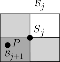
Figure 3: The interactive protocol: if $P$ is in the light gray regions, the verifier rejects. In this case, $P\prec S_{j}$, leading to ${\cal B}_{j+1}$ as shown in dark gray.

So now we describe how a single round works. the verifier (secretly) selects an index $i$ uniformly at random from $(0,n]$. Let $F(i)=\langle i,f(i)\rangle$. The prover and verifier jointly generate a nested sequence ${\cal B}_{1}\supset\cdots\supset{\cal B}_{k}$ of boxes all containing $F(i)$ and a sequence $S_{1},\ldots,S_{k}$ of points. For all $j$, $S_{j}$ is contained in ${\cal B}_{j}$. At the beginning of the $j$th round, ${\cal B}_{1},\ldots,{\cal B}_{j}$ and $S_{1},\ldots,S_{j-1}$ are already determined. (We initialize with ${\cal B}_{1}$ as a box containing all input points.) Now, the verifier selects some point $S_{j}$ inside ${\cal B}_{j}$. This is called a splitter for ${\cal B}_{j}$. The verifier compares $F(i)$ with $S_{j}$ and rejects if $F(i)$ is incomparable to $S_{j}$. (Refer to [fig:prot]Fig. 3.) If $F(i)\preceq S_{j}$, then the verifier declares ${\cal B}_{j+1}$ to be the box formed by the bottom-left corner of ${\cal B}_{j}$ and $S_{j}$. If $F(i)\succ S_{j}$, then ${\cal B}_{j+1}$ is the box formed by $S_{j}$ and the top-right corner of ${\cal B}_{j}$. This ends the $j$th round. If this process finally leads to a box ${\cal B}_{k}$ containing the single point $F(i)$, then the verifier accepts the index $i$.

Suppose ${\cal L}$ is some LIS. The prover can make the verifier accept whenever $F(i)$ belongs to ${\cal L}$ by always selecting $S_{i}$ so that $S_{i}\in{\cal L}\cap{\cal B}_{i}$. (Note that at each step the set ${\cal L}\cap{\cal B}_{i}$ is an LIS for the box ${\cal B}_{i}$.) We leave it to the reader to show that the prover cannot make the verifier to accept with probability higher than $|{\cal L}|/n={\tt lis}_{f}/n$.

The number of rounds of the protocol depends on how balanced the splitters selected by the prover are. A splitter $S_{i}$ is $\rho$-balanced in ${\cal B}_{i}$ if it does not belong to the leftmost or rightmost $\rho$ fraction of points of ${\cal B}_{i}$, which ensures that each successive box is reduced in size by a factor $1-2\rho$. This would bound the number of rounds by $O(\log n/\rho)$. We require that the prover select a $\rho$-balanced splitter for some $\rho=\Theta(\delta)$ (if there is such a splitter) and halt otherwise. Iimposing the $\rho$-balance requirement on the prover can decrease the probability of convincing the verifier by at most $\Theta(\rho)$).

Algorithmically searching for a splitter

Can we simulate this protocol by an algorithm? At first glance this seems impossible, since the prover has complete knowledge of the array, while the algorithm must “pay” for any information.

At each step, the all-knowing prover selects a $\rho$-balanced splitter in the current box that belongs to the LIS within that box. Since our algorithm does not know the LIS, it seems impossible to simulate this. But since we are only doing an approximation, we do not need the splitter to be on the LIS, we only need that the splitter belongs to an increasing sequence that is close to the LIS. How can we recognize such a splitter?

Let ${\cal B}_{j}$ be the current box being split and ${\cal L}_{j}$ be the LIS of ${\cal B}_{j}$. We say that an input point $P$ is a violation with a splitter $S$ if they are incomparable. A good splitter is one which is a violation with few points in ${\cal L}_{j}$. How few? If we can guarantee that the number of violations of the LIS with the splitter is at most $\gamma 0pt({\cal B})$, then the total error will be $\gamma 0pt({\cal B})$ times the number of rounds which is $O(\log n/\rho)$. The overall error will be a small fraction of $0pt({\cal B})$ if $\gamma$ is a small fraction of $\rho/\log n$.

It will be convenient in this informal discussion to assume that splitters are not necessarily input point (although it turns out that our algorithm will restrict its search for splitters to input points). We do not know what ${\cal L}_{j}$ is, so we look for a splitter $S$ with a much stronger property: $S$ has a total of $\gamma 0pt({\cal B})$ (input point) violations in ${\cal B}_{j}$. We call this a conservative splitter. This is a stronger requirement than what is needed for a good splitter because it includes violations of the splitter with points that are not on the LIS. If we can find a conservative splitter, it is safe to use it as the splitter in the interactive proof. Whether a candidate point is a conservative splitter for box ${\cal B}_{j}$ can be quickly (approximately) checked by estimating the fraction of violations that $i$ has within ${\cal B}_{j}$ by examining a small random sample of indices from ${\cal B}_{j}$. Furthermore, if a non-trivial fraction of points are conservative splitters, then one can be found and identified quickly by random sampling.

Thus conservative splitters are easy to find (if there are enough of them) and if one is found then we can use it to simulate the prover. Of course, there may not be enough conservative splitters for the random search algorithm to succeed; indeed there may be no conservative splitters. A new idea is required to deal with this problem: boosting the quality of the approximation.

Boosting the quality of approximation

Let us restart our quest for an algorithm from a different starting point: Given an algorithm that guarantees an additive $\delta n$-approximation to ${\tt lis}_{f}$, can we use it to get an additive $\delta^{\prime}$-approximation for some smaller $\delta^{\prime}$? If we could, then by using the known additive $1/2$-approximation algorithm as a starting point, we might be able to apply this error reduction method recursively to achieve any desired error.

Consider the following divide-and-conquer dynamic program for estimating the LIS of points in a box ${\cal B}$. Fix $s$ to be some (balanced) index in ${\cal B}$. Let $y$ be the value of some point in ${\cal B}$ and set $P=\langle s,y\rangle$. By varying $y$, we get different points $P$. Define the box ${\cal B}_{L}(P)$ formed by the bottom-left corner of ${\cal B}$ and $P$. Analogously, ${\cal B}_{R}(P)$ is formed by $P$ and the top-right corner of ${\cal B}$. Observe that ${\tt lis}({\cal B})=\max_{P}\{{\tt lis}({\cal B}_{L}(P))+{\tt lis}({\cal B}_{R}(P))\}$. This recurrence can be viewed as a dynamic program for ${\tt lis}({\cal B})$. Let ${\tt alis}({\cal B}_{L}(P))$ and ${\tt alis}({\cal B}_{R}(P))$ denote estimates obtained by running our base approximation algorithm on ${\cal B}_{L}(P)$ and ${\cal B}_{R}(P)$. We can maximize ${\tt alis}({\cal B}_{L}(P))+{\tt alis}({\cal B}_{R}(P))$ over $P$ to get an approximation for ${\tt lis}({\cal B})$ While it is too costly to search over all points $P$, a good approximation can be obtained by maximizing over a polylogarithmic sample from the points in ${\cal B}$. For the sake of this discussion, we will assume that the true maximizer $P^{*}$ can be determined. We denote the corresponding boxes ${\cal B}_{L}(P^{*})$ and ${\cal B}_{R}(P^{*})$ by ${\cal B}_{L}$ and ${\cal B}_{R}$.

An initial analysis suggests that we gain nothing from this. If ${\tt alis}({\cal B}_{L})$ is a $\delta 0pt({\cal B}_{L})$-additive approximation and ${\tt alis}({\cal B}_{R})$ is a $\delta 0pt({\cal B}_{R})$-additive approximation then the best we can say is that the sum is an additive $\delta(0pt({\cal B}_{L})+0pt({\cal B}_{R}))=\delta 0pt({\cal B})$ approximation to ${\tt lis}({\cal B})$, so we get no advantage.

However, if we make a subtle change in the notion of additive error, then an advantage emerges. Instead of measuring the additive approximation error as a multiple of $0pt({\cal B})$, we measure it as a multiple of ${\tt loss}({\cal B})=|{\cal B}\cap{\cal F}|-{\tt lis}({\cal B})$, where ${\cal F}=\{F(i):i\in[n]\}$ is the set of input points. Note that in general ${\tt loss}({\cal B})$ may be much smaller than $0pt({\cal B})$. So suppose we have an algorithm that whose approximation error is at most $\tau{\tt loss}({\cal B})$. Then the additive error of ${\tt alis}({\cal B}_{L})+{\tt alis}({\cal B}_{R})$ will be at most $\tau({\tt loss}({\cal B}_{L})+{\tt loss}({\cal B}_{R}))$, which may be significantly less than $\tau{\tt loss}({\cal B})$. If this can be bounded above by $\tau^{\prime}{\tt loss}({\cal B})$ for some $\tau^{\prime}<\tau$, the quality of approximation can be boosted.

The nice surprise is that ${\tt loss}({\cal B})-({\tt loss}({\cal B}_{L})+{\tt loss}({\cal B}_{R}))|=|{\cal B}\cap{\cal F}|-(|{\cal B}_{L}\cap{\cal F}|+|{\cal B}_{R}\cap{\cal F}|)$. This quantity is precisely the number of points in ${\cal B}\cap{\cal F}$ that are in violation with $P^{*}$. This gives the following dichotomy: if the number of such violations is at least $\mu|{\cal B}\cap{\cal F}|$ then we can take $\tau^{\prime}$ to be $(1-\mu)\tau$ and boost the quality of approximation from $\tau$ to $\tau^{\prime}$. Otherwise, the number of violations is less than $\mu|{\cal B}|$ and $P^{*}$ is a conservative splitter!

It is not clear how to apply this dichotomy to interleave the simulation of the interactive protocol and the boosting idea to get an algorithm. But there is a more significant difficulty. In the search for a good splitter we measured the number of violations as $\gamma 0pt({\cal B})$ and argued that $\gamma$ should be $O(1/\log n)$. For the recursive boosting to work efficiently, we measured the quality of the splitter by $\mu|{\cal B}|$ and for this we need $\mu$ to be at least $\Omega(1/\log\log n)$. Why? For each level of recursion, we can improve the additive approximation from $\tau$ to $\tau(1-\mu)$. So we will need $1/\mu$ levels of recursion to improve from $\delta$ to $\delta/2$. At each level of the recursion, we make at least $2$ recursive calls, for the left and right subproblems generated by any choice of a splitter. So the total number of iterated recursive calls is exponential in $1/\mu$. Since we want the running time to be $\log(n)^{O(1)}$, this leads to $\mu=\Omega(1/\log\log n)$.

For the interactive protocol simulation, splitters can have at most $O(|{\cal B}\cap{\cal F}|/\log n)$ violations inside ${\cal B}$, and for the boosting algorithm every (or nearly every) splitter has $\Omega(|{\cal B}\cap{\cal F}|/\log\log n)$ inside ${\cal B}$. So while the dichotomy seems promising, we have a huge gap from an algorithmic perspective.

Closing the dichotomy gap

We seek ways to close the gap in this dichotomy. Upon further consideration (and using past work in the area as a guide), it seems fruitful to modify the criterion for a good splitter. For a candidate splitter $P$ we relax the condition on the maximum number of violations $\gamma 0pt({\cal B})$ to $\mu|{\cal B}\cap{\cal F}|+\gamma 0pt({\cal B})$, where $\gamma$ will be $1/\textrm{poly}\log n$ and $\mu$ will be a small constant. (We strengthen this requirement by requiring that a similar condition holds for various subboxes of ${\cal B}$.) Note that this condition is weaker than the original condition on splitters. But we prove that it is good enough to simulate the interactive protocol.

Now for the other side of the dichotomy. Even if there is no good splitter satisfying this weaker condition, the above divide-and-conquer scheme might still fail to boost the quality of approximation. The boosting algorithm uses an index $s$ to divide the box ${\cal B}$ into two parts and then searches over different $y$ to maximize ${\tt alis}({\cal B}_{L})+{\tt alis}({\cal B}_{R})$. This is essentially solving a longest path problem on a 3-layer DAG. In the modified boosting algorithm we do analogous thing, but where we divide the box into a larger number of parts and solve a longest path problem on a DAG with more layers. The number of layers turns out to be $1/\gamma$, where $\gamma$ is the parameter in the relaxed definition of splitter.

These two ingredients - the simulation of the interactive protocol and the modified boosting algorithm - are combined together to give our algorithm. There are various parameters such as $\alpha,\mu,\gamma$ involved in the algorithm, and we must choose their values carefully. We also need to determine how many levels of boosting are required to get a desired approximation. A direct choice of parameters leads to a $(\log n)^{1/\delta}$ approximation algorithm. The better algorithm claimed in [thm:main]Thm. 1.1 is obtained by a more delicate version of the algorithm, which involves modifying the various parameters as the algorithm proceeds. This reduces the number of recursive calls needed for boosting from polylogarithmic in $n$ to a constant depending on $\delta$.

3 Preliminaries

3.1 Basic definitions

We write $\mathbb{N}$ for the set of nonnegative integers and $\mathbb{N}^{+}$ for the set of positive integers. We typically use interval notation $[a,b]$ and $(a,b]$ to denote intervals of nonnegative integers. Occasionally we also use interval notation to denote intervals of real numbers; the context should make it clear which meaning is intended.

Throughout this paper $n$ is an arbitrary but fixed positive integer and we refer to the set $(0,n]=\{1,\ldots,n\}$ as the index set. We let $f$ denote a fixed arbitrary function mapping $(0,n]$ to $\mathbb{N}^{+}$. Occasionally, we abuse notation and view 0 as an index. Also for convenience, we assume that we are given an upper bound ${\tt valbound}$ on the maximum of $f$. and define ${\rm range}(f)$ to be the set $[1,{\tt valbound}]$.

For $X\subseteq(0,n]$ we write $f(X)=\{f(x):x\in X\}$, and for $Y\subseteq{\rm range}(f)$ we write $f^{-1}(Y)=\{x\in[n]:f(x)\in Y\}$.

Points

As usual, $\mathbb{N}^{2}$ denotes the set of ordered pairs of nonnegative integers, which we call points. A point is denoted by $\langle a,b\rangle$ (rather than $(a,b)$, to avoid confusion with interval notation). The first coordinate of point $P$ is denoted $x(P)$ and is called the index of $P$. The second coordinate of $P$ is denoted $y(P)$ is called the value of $P$. We denote points by upper case letters, and sets of points by calligraphic letters.

The sets $X({\cal S})$ and $Y({\cal S})$

For a set ${\cal S}$ of points, we write $X({\cal S})$ for the set $\{x(P):P\in{\cal S}\}$ of indices of points of ${\cal S}$, and $Y({\cal S})$ for the set $\{y(P):P\in{\cal S}\}$ of values of points in ${\cal S}$.

The point $F(x)$, the set ${\cal F}$, and ${\cal F}$-points

For $x\in(0,n]$, $F(x)$ denotes the point $\langle x,f(x)\rangle$. We define ${\cal F}=\{F(x):x\in(0,n]\}$. We refer to points in ${\cal F}$ as ${\cal F}$-points.

Observe that for a set ${\cal S}$ of points, $F^{-1}({\cal S})\subseteq X({\cal S})$ is the set of indices $x$ for which $F(x)\in{\cal S}$. Since $F$ is a 1-1 function it follows that the sets $F^{-1}({\cal S})$ and ${\cal F}\cap{\cal S}$ are in 1-1 correspondence.

Relations $P\leq Q$, $P\prec Q$, $P\searrow Q$, $P\mathchoice{{\ooalign{$\displaystyle\searrow$\cr\hfil$\displaystyle*$\hfil\cr}}}{{\ooalign{$\textstyle\searrow$\cr\hfil$\textstyle*$\hfil\cr}}}{{\ooalign{$\scriptstyle\searrow$\cr\hfil$\scriptstyle*$\hfil\cr}}}{{\ooalign{$\scriptscriptstyle\searrow$\cr\hfil$\scriptscriptstyle*$\hfil\cr}}}Q$ and sets $P^{NE}$, $P^{NW}$, $P^{SE}$,$P^{SW}$

For points $P,Q$,

$P\leq Q$

means $x(P)\leq x(Q)$ and $y(P)\leq y(Q)$

$P\prec Q$

means $x(P)<x(Q)$ and $y(P)\leq y(Q)$.

$P\searrow Q$

means $x(P)<x(Q)$ and $y(P)>y(Q)$.

$P\mathchoice{{\ooalign{$\displaystyle\searrow$\cr\hfil$\displaystyle*$\hfil\cr}}}{{\ooalign{$\textstyle\searrow$\cr\hfil$\textstyle*$\hfil\cr}}}{{\ooalign{$\scriptstyle\searrow$\cr\hfil$\scriptstyle*$\hfil\cr}}}{{\ooalign{$\scriptscriptstyle\searrow$\cr\hfil$\scriptscriptstyle*$\hfil\cr}}}Q$

means $x(P)\leq x(Q)$ and $y(P)>y(Q)$.

Observe that for points $P,Q$ with $x(P)\neq x(Q)$, for example, if $P,Q$ are distinct points of ${\cal F}$, then the conditions $x(P)\leq x(Q)$ and $x(P)\prec x(Q)$ are equivalent, and the conditions $P\searrow Q$ and $P\mathchoice{{\ooalign{$\displaystyle\searrow$\cr\hfil$\displaystyle*$\hfil\cr}}}{{\ooalign{$\textstyle\searrow$\cr\hfil$\textstyle*$\hfil\cr}}}{{\ooalign{$\scriptstyle\searrow$\cr\hfil$\scriptstyle*$\hfil\cr}}}{{\ooalign{$\scriptscriptstyle\searrow$\cr\hfil$\scriptscriptstyle*$\hfil\cr}}}Q$ are equivalent.

For a point $P$, we define the following sets. Refer to [fig:position]Fig. 4.

$P^{NW}$

(for northwest) The set of points $Q$ such that $Q\mathchoice{{\ooalign{$\displaystyle\searrow$\cr\hfil$\displaystyle*$\hfil\cr}}}{{\ooalign{$\textstyle\searrow$\cr\hfil$\textstyle*$\hfil\cr}}}{{\ooalign{$\scriptstyle\searrow$\cr\hfil$\scriptstyle*$\hfil\cr}}}{{\ooalign{$\scriptscriptstyle\searrow$\cr\hfil$\scriptscriptstyle*$\hfil\cr}}}P$.

$P^{SW}$

(for southwest) The set of points $Q$ such that $Q\leq P$.

$P^{NE}$

(for northeast) The set of points $Q$ such that $P\prec Q$.

$P^{SE}$

(for southeast) The set of points $Q$ such that $P\searrow Q$.

Figure 4: The various positions and sets relative to point $P$. $Q$ denotes a hypothetical point in the respective region.

There is an asymmetry in these definitions: For example one might expect that $Q\in P^{NE}$ would be equivalent to $P\in Q^{SW}$ but this is not the case. Notice that this asymmetry disappears if $x(P)\neq x(Q)$. One reason to define the sets this way is so that for each point $P$, the sets $P^{NW}$,$P^{NE}$, $P^{SW}$, $P^{SE}$ partition $\mathbb{N}^{2}$.

Relations $P\sim Q$ ($P$ is comparable to $Q$) and $P\not\sim Q$ ($P$ is a violation with $Q$)

For $P,Q\in{\cal F}$ we define:

$P\sim Q$

means that $P$ and $Q$ are comparable, i.e., $P\leq Q$ or $Q\leq P$ .

$P\not\sim Q$

means that $P$ and $Q$ are a incomparable or a violation, i.e., either $P\searrow Q$ or $Q\searrow P$ .

We emphasize that we only use these terms in the case that $P$ and $Q$ are ${\cal F}$-points. Since ${\cal F}$-points have distinct indices, the distinctions between $\leq$ and $\prec$, and between $\searrow$ and $\textstyle\searrow$ $\textstyle*$ disappear.

Index intervals

A set of consecutive indices is called an index interval. An index interval is usually written using the notation $(a,b]=\{a+1,\ldots,b\}$. For an index interval $I$, we define indices $x_{L}(I)$ and $x_{R}(I)$, the left and right endpoints of $I$ so that $I=(x_{L}(I),x_{R}(I)]$. Note $x_{R}(I)\in I$ but $x_{L}(I)\not\in I$.

Value intervals

A value interval refers to an integer subinterval $[c,d]$ of ${\rm range}(f)$. For value intervals we always use closed interval notation. For a value interval $J$ we define indices $y_{B}(J)$ and $y_{T}(J)$, the top and bottom endpoints of $J$ such that $J=[y_{B}(J),y_{T}(J)]$. Thus, in contrast with index intervals, $J$ contains both of its endpoints.

Box

A box ${\cal B}$ is the Cartesian product of a nonempty index interval $I$ and a nonempty value interval $J$.

Using the notation described above, we have ${\cal B}=X({\cal B})\times Y({\cal B})$, $X({\cal B})=(x_{L}(X({\cal B})),x_{R}(X({\cal B}))]$, and $Y({\cal B})=[y_{B}(Y({\cal B}),y_{T}(Y({\cal B}))]$. To simplify notation we define $x_{L}({\cal B})=x_{L}(X({\cal B}))$ and analogously $x_{R}({\cal B}),y_{B}({\cal B}),y_{T}({\cal B})$. Thus $X({\cal B})=(x_{L}({\cal B}),x_{R}({\cal B})]$ and $Y({\cal B})=[y_{B}({\cal B}),y_{T}({\cal B})]$. We also define the bottom-left point of ${\cal B}$, $P_{BL}({\cal B})=\langle x_{L}({\cal B}),y_{B}({\cal B})\rangle$ and the top-right point of ${\cal B}$, $P_{TR}({\cal B})=\langle x_{R}({\cal B}),y_{T}({\cal B})\rangle$. (Note that under these definitions $P_{BL}({\cal B})\not\in{\cal B}$ since $x_{L}({\cal B})\not\in X({\cal B})$.)

If $Q,R$ are points with $Q\prec R$, the box spanned by $Q,R$, denoted $Box(Q,R)$ is the box having $P_{BL}({\cal B})=Q$ and $P_{TR}({\cal B})=R$. It is easy to see that $Box(Q,R)=\{P:Q\prec P\leq R\}$

Grids

A grid $\Gamma$ is any Cartesian product $I\times J$ where $I$ is a set of indices and $J$ is a set of values. Thus $\Gamma$ is a grid if and only if $\Gamma=X(\Gamma)\times Y(\Gamma)$. A box is the special case of a grid in which both $X(\Gamma)$ and $Y(\Gamma)$ are intervals.

We refer to the sets of the form $\{x\}\times Y(\Gamma)$ for $x\in X(\Gamma)$ as columns of $\Gamma$ and sets of the form $X(\Gamma)\times\{y\}$ for $y\in Y(\Gamma)$ as rows of $\Gamma$.

The universe ${\cal U}$ and the universal grid $\Gamma({\cal U})$

The universe ${\cal U}$ is the box $(0,n]\times{\rm range}(f)$. The universal grid is the grid $(0,n]\times F(0,n]$. This is the smallest grid that contains ${\cal F}$, and its size is at most $n^{2}$. Every point that is encountered in any of our algorithms belongs to the universal grid.

width

The width of an interval $I$, denoted $0pt(I)$, is $|I|=x_{R}(I)-x_{L}(I)$. Similarly, for a box ${\cal B}$, $0pt({\cal B})$ is equal to $|X({\cal B})|=x_{R}({\cal B})-x_{L}({\cal B})$.

Relation $\triangleleft$ on index intervals and boxes

• For index intervals $I_{1},I_{2}$ we write $I_{1}\triangleleft I_{2}$ if $x_{R}(I_{1})=x_{L}(I_{2})$. It follows that $I_{1}\cap I_{2}=\emptyset$ and $I_{1}\cup I_{2}$ is equal to the index interval $(x_{L}(I_{1}),x_{R}(I_{2})]$. In particular this implies that $x_{1}<x_{2}$ for all $x_{1}\in I_{1}$ and $x_{2}\in I_{2}$.

• For boxes ${\cal B}_{1},{\cal B}_{2}$ we write ${\cal B}_{1}\triangleleft{\cal B}_{2}$ to mean $P_{TR}({\cal B}_{1})=P_{BL}({\cal B}_{2})$. This is equivalent to $X({\cal B}_{1})\triangleleft X({\cal B}_{2})$ and $y_{T}({\cal B}_{1})=y_{B}({\cal B}_{2})$. In particular, this implies ${\cal B}_{1}\cap{\cal B}_{2}=\emptyset$ and $P_{1}\prec P_{2}$ for all $P_{1}\in{\cal B}_{1}$ and $P_{2}\in{\cal B}_{2}$.

Box sequences

A box sequence is a list of boxes such that each successive box is entirely to the right of the previous. We use the notation $\vec{{\cal B}}$ to denote a box sequence. We write ${\cal B}\in\vec{{\cal B}}$ to mean that the box ${\cal B}$ appears in $\vec{{\cal B}}$.

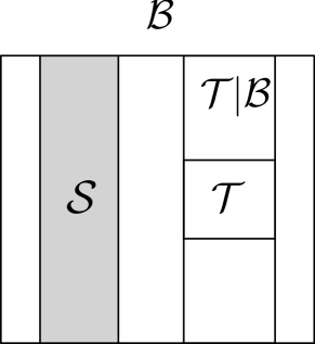
(a) ${\cal B}$-strip

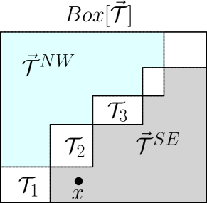
(b) Box chains

            

Figure 5: (a) ${\cal S}$ is a ${\cal B}$-strip. The figure also shows the strip ${\cal T}|{\cal B}$ for box ${\cal T}$. (b) The box chain $\vec{\cal T}$: The boxes ${\cal T}_{1},{\cal T}_{2},\ldots$ form a chain. The box $\vec{{\cal T}}[x]$ is ${\cal T}_{2}$. The regions $\vec{{\cal T}}^{NW}$ and $\vec{{\cal T}}^{SE}$ are shaded.

${\cal B}$-strips and ${\cal B}$-strip decompositions

If ${\cal B}$ is a box, a ${\cal B}$-strip is a subbox ${\cal S}$ of ${\cal B}$ such that $Y({\cal S})=Y({\cal B})$. Thus a ${\cal B}$-strip has the same vertical extent as ${\cal B}$ and is specified relative to ${\cal B}$ by its index set $X({\cal S})$. If $I\subseteq X({\cal B})$ is an index interval then $I|{\cal B}$ denotes the ${\cal B}$-strip with index set $I$. Similarly if ${\cal T}$ is a subbox of ${\cal B}$ then ${\cal T}|{\cal B}$ denotes the strip $X({\cal T})|{\cal B}$. Refer to [fig:strip]Fig. 5a.

A ${\cal B}$-strip decomposition is a partition of ${\cal B}$ into strips. A ${\cal B}$-strip decomposition into $r$ strips is specified by a sequence $x_{0}=x_{L}({\cal B})<x_{1}<\cdots<x_{r}=x_{R}({\cal B})$, where the $j$th strip is $(x_{j-1},x_{j}]|{\cal B}$. We use the sequence notation $\vec{{\cal S}}$ to denote a ${\cal B}$-strip decomposition in the natural left-to-right order.

In particular if $\Gamma\subset{\cal B}$ is a grid then $\Gamma$ naturally defines a strip decomposition of ${\cal B}$ obtained by taking the strips that end at successive columns of $\Gamma$ with the final strip ending at $x_{R}({\cal B})$.

Increasing point sequences and Box Chains

A set of points ${\cal P}$ that can be ordered so that $P_{0}\prec\cdots\prec P_{k}$ is called an increasing point sequence or simply increasing sequence. If ${\cal S}$ is a set of points then an ${\cal S}$-increasing point sequence is an increasing sequence whose points all belong to ${\cal S}$.

A box chain $\vec{{\cal T}}$ is a box sequence $\vec{{\cal T}}=({\cal T}_{1},\ldots,{\cal T}_{k})$ satisfying ${\cal T}_{1}\triangleleft\cdots\triangleleft{\cal T}_{k}$. Refer to [fig:boxchain]Fig. 5b for the following definitions.

• There is a one-to-one correspondence between increasing point sequences and box chains which maps the increasing sequence ${\cal P}$ with points $P_{0}\prec P_{1}\prec\ldots\prec P_{k}$ to the box chain $\vec{{\cal T}}$ given by $Box(P_{0},P_{1})\triangleleft\cdots\triangleleft Box(P_{k-1},P_{k})$. We refer to ${\cal P}$ as the increasing sequence associated to box chain $\vec{{\cal T}}$. If $\vec{{\cal T}}$ is a box chain, we write ${\cal P}(\vec{{\cal T}})$ for the associated increasing point sequence and ${\cal P}^{\circ}(\vec{{\cal T}})$ for the interior increasing sequence associated to $\vec{{\cal T}}$, which excludes the first and last points $P_{0}$ and $P_{k}$.

• The box $Box[\vec{{\cal T}}]$ spanned by $\vec{{\cal T}}$ is the smallest box containing $\vec{{\cal T}}$. If $P_{0},\cdots,P_{k}$ is the increasing point sequence associated to $\vec{{\cal T}}$ then $Box[\vec{{\cal T}}]=Box(P_{0},P_{k})$.

• If $\vec{{\cal T}}$ spans box ${\cal B}$ then for each $x\in X({\cal B})$ there is a unique box ${\cal T}\in\vec{{\cal T}}$ such that $x\in X({\cal T})$. This box is denoted $\vec{{\cal T}}[x]$

• Given a strip decomposition $\vec{{\cal S}}$ of ${\cal B}$, a box chain $\vec{{\cal T}}$ is compatible with $\vec{{\cal S}}$ if $\vec{{\cal S}}$ is composed of strips ${\cal T}|{\cal B}$ for ${\cal T}\in\vec{{\cal T}}$. In this case, the box spanned by $\vec{{\cal T}}$ has the form $X({\cal B})\times Y^{\prime}$ where $Y^{\prime}\subseteq Y({\cal B})$.

• If $\vec{{\cal T}}$ is a box chain spanning box ${\cal B}$, then $\vec{{\cal T}}$ naturally defines a partition of ${\cal B}$ into three sets: $\vec{{\cal T}}^{\cup}$, $\vec{{\cal T}}^{NW}$ (for northwest) and $\vec{{\cal T}}^{SE}$ (for southeast), where:

  • $\vec{{\cal T}}^{\cup}=\bigcup_{{\cal T}\in\vec{{\cal T}}}{\cal T}$. Equivalently, $\vec{{\cal T}}^{\cup}={\cal B}\cap\bigcap_{P\in{\cal P}(\vec{{\cal T}})}(P^{SW}\cup P^{NE})$.

  • $\vec{{\cal T}}^{NW}={\cal B}\cap\bigcup_{P\in{\cal P}(\vec{{\cal T}})}P^{NW}$.

  • $\vec{{\cal T}}^{SE}={\cal B}\cap\bigcup_{P\in{\cal P}(\vec{{\cal T}})}P^{SE}$.

3.2 Increasing sequences and the functions lis and loss

A set $X\subseteq(0,n]$ of indices is said to be $F$-increasing if the set $F(X)=\{F(x):x\in X\}$ is an increasing point sequence. For a box ${\cal B}$ we say that $X$ is $(F,{\cal B})$-increasing if it is $F$-increasing and $F(X)\subseteq{\cal B}$. If $\vec{{\cal B}}$ is a box chain we say that $X$ is $(F,\vec{{\cal B}})$-increasing if it is $F$-increasing and $F(X)\subseteq\vec{{\cal B}}^{\cup}$.

• ${\tt lis}({\cal B})={\tt lis}_{f}({\cal B})$ is the size of a longest increasing (point) sequence (LIS) contained in ${\cal B}$, which is also the size of the largest $(F,{\cal B})$-increasing set.

• ${\tt loss}({\cal B})=|{\cal B}\cap{\cal F}|-{\tt lis}({\cal B})$, i.e. ${\tt loss}({\cal B})$ is the smallest number of ${\cal F}$-points in ${\cal B}$ that must be deleted so that the remaining points of ${\cal B}\cap{\cal F}$ form an increasing sequence.

3.3 The LIS approximation problem

We develop an algorithm ${\rm{\bf ApproxLIS}}$ that takes as input a function $f$ and box ${\cal B}$ and outputs an approximation ${\rm{\bf ApproxLIS}}({\cal B})$ to ${\tt lis}({\cal B})$. The required quality of approximation is specified by input parameters $\overline{\tau}$ and $\overline{\delta}$. The algorithm is recursive and calls itself with different choices of these input parameters. To prevent confusion, the symbols $\overline{\tau}$ and $\overline{\delta}$ denote the initial setting, while $\tau$ and $\delta$ are used to generically refer to these parameters in the algorithm.

In our analysis we will require a carefully chosen measure of the quality of the estimate ${\rm{\bf ApproxLIS}}({\cal B})$. For $\overline{\tau},\overline{\delta}\in(0,1)$ we say that ${\rm{\bf ApproxLIS}}$ is a $(\overline{\tau},\overline{\delta})$-approximation to ${\tt lis}$ on box ${\cal B}$ provided that:

$$|{\rm{\bf ApproxLIS}}({\cal B})-{\tt lis}({\cal B})|\leq\overline{\tau}{\tt loss}({\cal B})+\overline{\delta}0pt({\cal B}).$$

A few remarks:

• A $(0,\overline{\delta})$-approximation is an additive $\overline{\delta}0pt({\cal B})$-approximation to ${\tt lis}({\cal B})$. Since ${\tt loss}({\cal B})\leq 0pt({\cal B})$ a $(\overline{\tau},\overline{\delta})$-approximation is also an additive $(\overline{\tau}+\overline{\delta})$-approximation.

• Our initial goal is to get a good additive approximation, so the reader may wonder why we introduce the parameter $\overline{\tau}$. Separating the error into these two parts is important for the analysis of our algorithm. Our algorithm is recursive. The value of $\tau$ in the base algorithm is very large (essentially infinite), but we have the freedom to choose $\delta$ to be very small. Each level of recursion shrinks $\tau$, at the cost of making $\delta$ larger. By applying enough recursive levels, we can make the final $\tau$ less than the desired bound of $\overline{\tau}$. By starting with a small initial $\delta$, we can keep the final $\delta$ at most $\overline{\delta}$. This ensures the final algorithm is a $\overline{\tau}+\overline{\delta}$-additive approximation.

• We refer to the quantity $\tau{\tt loss}({\cal B})$ as the primary error and to $\delta 0pt({\cal B})$ as the secondary error.

4 The main theorems

We present two polylogarithmic time approximation algorithms for LIS, which we refer to as the basic algorithm and the improved algorithm. The basic algorithm is somewhat simpler (though still fairly involved) while the improved algorithm enhances the basic algorithm to give significantly better running time. For the running time of the basic algorithm, the exponent of $\log n$ is $\Theta(1/\overline{\tau})$. For the improved version, the exponent of $\log n$ is a constant independent of the error parameters $\overline{\tau}$ and $\overline{\delta}$.

Theorem 4.1.

There is a randomized algorithm ${\rm{\bf BasicMain}}$ that:

• takes as input an integer $n$, an array $f$ of length $n$ and an error parameter $\overline{\tau}\in(0,1)$,

• runs in time $(\log n)^{O(1/\overline{\tau})}$, and

• outputs a value that, with probability at least $1-n^{-\Omega(\log n)}$, is a $(\overline{\tau},\frac{5}{\overline{\tau}\log n})$-approximation to ${\tt lis}({\cal B})$.

Our improved algorithm gives:

Theorem 4.2.

There is a randomized algorithm ${\rm{\bf ImprovedMain}}$ that:

• takes as input an integer $n$, an array $f$ of length $n$ and error parameters $\overline{\tau},\overline{\delta}\in(0,1)$,

• runs in time $(1/\overline{\delta}\overline{\tau})^{O(1/\overline{\tau})}(\log n)^{c}$, and

• outputs a value that, with probability at least $3/4$, is a $(\overline{\tau},\overline{\delta})$-approximation to ${\tt lis}_{f}$.

In the second theorem the probability of error is 1/4, as compared to $n^{-\Omega(\log n)}$ in the first. It just happens that the analysis of the first algorithm gives a better error probability. As we noted in the introduction, this difference is not significant: we can always reduce the error probability of the second algorithm to any desired $\varepsilon>0$ by the standard trick of doing $O(\log(1/\varepsilon)$ independent trials of the algorithm, and outputing the median of the trials.

We deduce [thm:main]Thm. 1.1 and [thm:dist]Thm. 1.2 from [thm:alg2]Thm. 4.2.

[thm:dist]Thm. 1.2 requires a few calculations.

Proof 4.3 (of [thm:main]Thm. 1.1).

A $(\overline{\tau},\overline{\delta})$-approximation is also an additive $\overline{\tau}+\overline{\delta}$ approximation. Given a desired additive error $\delta$ in [thm:main]Thm. 1.1, we set $\overline{\delta}=\overline{\tau}=\delta/2$ and run ${\rm{\bf ImprovedMain}}$. [thm:alg2]Thm. 4.2 gives us the desired guarantee.

Proof 4.4 (of [thm:dist]Thm. 1.2).

For convenience, we will assume that ${\rm{\bf ImprovedMain}}$ has an error of $n^{-\Omega(\log n)}$. (Since we will make at most $\textrm{poly}(n)$ runs of ${\rm{\bf ImprovedMain}}$ and can union bound, we henceforth assume no error.) Suppose we run ${\rm{\bf ImprovedMain}}$ with parameters $\overline{\tau},\overline{\delta}$ and $a$ is the estimate. Then, $|n-a-{\tt loss}_{f}|\leq\overline{\tau}{\tt loss}_{f}+\overline{\delta}n$. We divide by $n$, note that $\varepsilon_{f}={\tt loss}_{f}/n$ and denote $b=1-a/n$. Hence, $b\in[\varepsilon_{f}(1-\overline{\tau})-\overline{\delta},\varepsilon_{f}(1+\overline{\tau})+\overline{\delta}]$. Rearranging, $\varepsilon_{f}\in[(b-\overline{\delta})/(1+\overline{\tau}),(b+\overline{\delta})/(1-\overline{\tau})]$. For convenience, we denote this interval by $[b_{1},b_{2}]$.

Our aim is to choose $\overline{\tau}$ and $\overline{\delta}$ such that $b_{2}/b_{1}\leq(1+\tau)$. Suppose we set $\overline{\tau}=q\cdot\tau$ and $\overline{\delta}\leq q\cdot\overline{\tau}\varepsilon_{f}$, for some sufficiently small absolute constant $q$. Then,

$$\frac{(b+\overline{\delta})/(1-\overline{\tau})}{(b-\overline{\delta})/(1+\overline{\tau})}=\frac{(b+\overline{\delta})(1+\overline{\tau})}{(b-\overline{\delta})(1-\overline{\tau})} \leq \frac{(\varepsilon_{f}(1+\overline{\tau})+2q\cdot\overline{\tau}\varepsilon_{f})(1+\overline{\tau})}{(\varepsilon_{f}(1-\overline{\tau})-2q\cdot\overline{\tau}\varepsilon_{f})(1-\overline{\tau})}$$

$$\leq \frac{(1+q(1+2q)\tau)(1+q\tau)}{(1-q(1-2q)\tau)(1-q\tau)}\leq 1+\tau.$$

But the value of $\varepsilon_{f}$ is not known in advance. We fix $\overline{\tau}=q\cdot\tau$ and run ${\rm{\bf ImprovedMain}}$ iteratively where the value of $\overline{\delta}$ during the $j$th run is $\overline{\tau}/2^{j}$. The algorithm will terminate before $\overline{\delta}\leq q\cdot\overline{\tau}\varepsilon_{f}/2$. The running time is dominated by that of the last iteration, which is $(1/\tau\varepsilon_{f})^{O(1/\tau)}(\log n)^{c}$.

5 Algorithmic and analytical building blocks

We present some procedures used in our algorithms, and some analytic tools we’ll need. First we establish some conventions and review basic tail bounds that will be useful in analyzing the use of randomness in our algorithms We define the notion of a good splitter of a box and present a subroutine for finding splitters. We present the important dichotomy lemma that roughly says: if there are few good splitters in a box ${\cal B}$ then ${\tt loss}({\cal B})$ must be a non-trivial fraction of $|{\cal B}\cap{\cal F}|$. We present a simple subroutine that given a box constructs a grid inside it that is suitably representative of the box.

5.1 Conventions for random bits

Random sampling is needed in the following procedures:

• The procedures ${\rm{\bf FindSplitter}}$, ${\rm{\bf BuildGrid}}$ which are presented later in this section. We refer to the random bits used in these procedures as secondary random bits.

• The main procedure ${\rm{\bf ApproxLIS}}$ which is presented in [sec:first algorithm]§6. The random bits used in this procedure are called the primary random bits.

All procedures depend on the function $f$. We treat the function $f$ as fixed, so the dependence on $f$ is implicit. The other arguments to these procedures are boxes, indices, and auxiliary precision and error parameters. We can enumerate the possible arguments to each of these procedures. Indices have $n$ possible values, and boxes always have their corners on the universal grid, so there are at most $n^{4}$ of them. The auxiliary parameters will be from a restricted set of size at most $((\log n)/\tau)^{O(1)}$ where $\tau$ is the primary error parameter.

For purposes of analysis, we imagine that before running the algortihm we pregenerate all of the random bits needed for each procedure and each possible set of arguments for the procedure, Once all of these bits are (conceptually) fixed, the running of the algorithm is deterministic. This viewpoint has three advantages for us.

1. In our overall algorithm, the same procedure may be called multiple times with the same arguments. For each such call, we use the same sequence of random bits, as generated at the outset of the algorithm. Therefore, every such duplicate call produces the same output.

2. The randomized procedure ${\rm{\bf Classify}}$ (defined in Section) will itself be run on a few randomly chosen indices. In the analysis, we need to reason about the output of ${\rm{\bf Classify}}$ on all inputs, not just the ones evaluated by the algorithm. By generating random bits for every possible call to a procedure, the output of ${\rm{\bf Classify}}$ can be seen as fixed on all possible inputs. If the random bits were not fixed in advance, then the output of ${\rm{\bf Classify}}$ on a new input is a random variable. Both points of view lead to the same mathematical conclusions, but viewing the randomness as fixed from the beginning simplifies the analysis.

3. In the analysis, we identify some useful (deterministic) assumptions of the ensemble of all of the random bits. The main analysis shows that if the ensemble of random bits satisfies these assumptions, then the output of our algorithm is guaranteed to have the right properties. This involves no probabilistic reasoning. Probabilistic arguments are only required to show that these two assumptions hold with very high probability over the choice of the ensemble of random bits.

The pre-generation of random bits is, of course, simply an analytical device. Since we want our algorithm to be fast, we cannot afford to generate all of bits in advance. So we generate random bits only as we need them, and only for those choices of parameters to procedures that actually arise. Once we evaluate a procedure with a given set of arguments, we record the input parameters and output. If the same procedure is called again with the same arguments, we return the same value. It is evident that this online approach to generating randomness produces the same distribution over executions and outputs as the inefficient offline approach. Hence, we execute the online algorithm, but use the offline viewpoint for analysis.

5.2 Tail bounds for sums of random variables

We recall a version of the Chernoff-Hoeffding bound for sums of random variables:

Proposition 1.

[Hoe63] Let $X_{1},\ldots,X_{n}$ be independent random variables with $X_{i}\in[a_{i},b_{i}]$ and $\mu_{i}=\mathbb{E}[X_{i}]$ and $\mu=\sum_{i}\mu_{i}$. Then for any $T>0$:

$${\rm Pr}[\sum_{i}X_{i}-\mu\geq T] \leq e^{-2T^{2}/\sum_{i}(b_{i}-a_{i})^{2}}$$

$${\rm Pr}[\sum_{i}X_{i}-\mu\leq-T] \leq e^{-2T^{2}/\sum_{i}(b_{i}-a_{i})^{2}}.$$

A standard application of is to bound the probability of error when estimating the size of a subpopulation within a given population. For a finite set $X$, a random sample of size $m$ from a set $X$ means a sequence $x_{1},\ldots,x_{m}$ of elements each drawn uniformly and independently from $X$.

Proposition 2.

Let $X$ be an index interval and $\gamma\in[0,1]$ and $s\in\mathbb{N}^{+}$. Let $A\subseteq X$ be fixed. For a random sample $x_{1},\ldots,x_{s}$ from $X$, let $r$ denote the fraction of points that belong to $A$. Then $\Pr[|r-\frac{|A|}{|X|}|\geq\gamma]\leq 2e^{-2\gamma^{2}s}$.

We will also need the following upper tail bound:

Proposition 3.

(Theorem 1, Eq. (1.8) in [DP09]) Let $X=\sum_{i}X_{i}$, where $X_{i}$’s are independently distributed in $[0,1]$. If $T>2e\hbox{\bf E}[X]$, then ${\rm Pr}[X>T]\leq 2^{-T}$.

5.3 Splitters and the subroutine ${\rm{\bf FindSplitter}}$

A basic operation in our algorithm is to take a box ${\cal T}$ and choose an index $s\in F^{-1}({\cal T})$, that is used to “split” the box ${\cal T}$ into the two boxes $Box(P_{BL}({\cal T}),F(s))$ and $Box(F(s),P_{TR}({\cal T}))$. This gives a box chain of size two spanning ${\cal T}$. For this reason, the index $s\in F^{-1}({\cal T})$ is called a splitter for ${\cal T}$; we also refer to the point $\langle s,f(s)\rangle$ as a splitter. Note that $s>x_{L}({\cal T})$ for all $s\in F^{-1}({\cal T})$ and therefore $Box(P_{BL}({\cal T}),F(s))$ is always a nonempty box. It could happen that $s=x_{R}({\cal T})$, in which case $Box(F(s),P_{TR}({\cal T}))$ is a trivially empty box. In this case we say that the splitter is degenerate; any other splitter is said to be nondegenerate.

We give a subroutine that, given a pair of boxes ${\cal T}\subseteq{\cal B}$, looks for a “useful” splitter $s$ for ${\cal T}$ with $F(s)\in{\cal T}$. We require a splitter to be balanced and safe (in a precise sense to be specified). Roughly, a balanced splitter is not too close to either the left or right edge of ${\cal T}$ (and in particular is not degenerate). A splitter is safe if most ${\cal F}$-points of ${\cal T}|{\cal B}$ are comparable to $F(s)$.

The definitions in this section are inspired by the classic ideas of inversion counting [EKK⁺00, ACCL07] for estimating the distance to monotonicity.

We begin by formally defining balanced indices.

Definition 5.1.

For a box ${\cal T}$ and $\rho\in[0,1]$, an index $x$ is said to be $\rho$-balanced in ${\cal T}$ if $x-x_{L}({\cal T})$ and $x_{R}({\cal T})-x$ are both at least $\rho 0pt({\cal T})$, and is $\rho$-unbalanced otherwise.

It follows that the number of $\rho$-balanced indices is at least $\lfloor(1-2\rho)0pt({\cal T})\rfloor$ and the number of $\rho$-unbalanced indices is at most $2\rho 0pt({\cal T})+1$. Excluding the degerate splitter $x_{R}({\cal T})$ we get:

Proposition 4.

For any $\rho>0$, the number of nondegenerate $\rho$-unbalanced splitters of ${\cal T}$ is at most $2\rho 0pt({\cal T})$.

The definition of safe has several parameters and “moving parts” and some preliminary discussion may be helpful. The definition involves three parameters: a box ${\cal R}$, a real number $\mu\in(0,1)$ and a positive real number $L$. The notion of safety is expressed by saying that $s$ is a $(\mu,L)$-safe splitter for ${\cal R}$. The requirements are that $s$ pass a collection of tests, one for each substrip ${\cal S}$ of ${\cal R}$ that is adjacent to $s$ in the following sense: either the maximum index in $X({\cal S})$ is $s-1$ or the minimum index is $s+1$. The requirement corresponding to substrip ${\cal S}$ of ${\cal R}$ is that the number of ${\cal F}$-points inside of ${\cal S}$ that are in violation with $F(s)$ should be “not too large” compared with the total number of ${\cal F}$-points inside of ${\cal S}$: specifically it should be at most $L+\mu|{\cal F}\cap{\cal S}|$.

Definition 5.2.

This is a series of definitions used to formalize safeness of splitters.

• $viol(s,{\cal S})$: This is the number of points $P\in{\cal S}\cap{\cal F}$ that are in violation with $F(s)$.

• $Z(s,{\cal S}):=viol(s,{\cal S})-\mu|{\cal F}\cap{\cal S}|$.

• $Z_{x}(s,{\cal S})$: This is defined for index $x\in X({\cal S})$. Suppose $F(x)\in{\cal S}$. If $F(x)\sim F(s)$, $Z_{x}(s,{\cal S})=-\mu$ and if $F(x)\not\sim F(s)$, $Z_{x}(s,{\cal S})=1-\mu$. If $F(x)\not\in{\cal S}$, $Z_{x}(s,{\cal S})$ is 0. Note that $Z(s,{\cal S})=\sum_{x\in X({\cal S})}Z_{x}(s,{\cal S})$.

• $(\mu,L)$-accepting: A strip ${\cal S}$ is $(\mu,L)$-accepting for $s$ if $Z(s,{\cal S})\leq L$ and is $(\mu,L)$-rejecting for $s$ otherwise.

• Adjacent strips: A strip ${\cal S}$ is said to be adjacent to $s$ if either $x_{L}({\cal S})=s$ (i.e. the lowest index in $X({\cal S})$ is $s+1$) or $x_{R}({\cal S})=s-1$ (the highest index in $X({\cal S})$ is $s-1$).

• $(\mu,L)$-unsafe: We say that $s$ is $(\mu,L)$-unsafe for ${\cal R}$ if there is some ${\cal R}$-strip ${\cal S}$ that is adjacent to $s$ and $(\mu,L)$-rejecting for $s$.

• $(\mu,L)$-safe:We say that $s$ is $(\mu,L)$-safe for ${\cal R}$ if every ${\cal R}$-strip ${\cal S}$ that is adjacent to $s$ is $(\mu,L)$-accepting for $s$. We remark that the $(\mu,L)$-safe and $(\mu.L)$-unsafe indices for ${\cal R}$ partition the set of splitters of ${\cal R}$.

With this preamble, we can state the main definition of adequate splitters.

Definition 5.3.

Let ${\cal T}\subseteq{\cal B}$ be a pair of boxes and $\mu,\rho\in(0,1)$ and $L>0$ . A splitter $s\in X({\cal T})$ is $(\mu,L,\rho)$-adequate for ${\cal T},{\cal B}$ if:

• $F(s)\in{\cal T}$

• $s$ is $(\mu,L)$-safe for ${\cal T}|{\cal B}$

• $s$ is $\rho$-balanced in ${\cal T}$.

We describe a procedure ${\rm{\bf FindSplitter}}$ that takes as input a pair of boxes ${\cal T}\subseteq{\cal B}$ and parameters $\rho,\mu$ and $L\geq 1$ and searches for such a splitter. The procedure returns a pair $(splitter\_found,s)$ where $splitter\_found$ is set to TRUE or FALSE and $s\in X({\cal T})$.

We say that an execution of ${\rm{\bf FindSplitter}}$ on input $({\cal T},{\cal B},\mu,L,\rho)$ is reliable if the following holds:

• If ${\cal T}$ has at least $\rho 0pt({\cal B})$ splitters that are $(\mu,L,\rho)$-adequate for ${\cal T},{\cal B}$ then $splitter\_found$ is set to TRUE.

• If $splitter\_found={\tt TRUE}$ then $s$ is a $(\mu,2L,\rho)$-adequate splitter for ${\cal T},{\cal B}$. (Note that here we relax the parameter $L$ to $2L$.)

An execution where either of these two conditions fails is called unreliable. The procedure ${\rm{\bf FindSplitter}}$ is designed so that each execution is reliable with high probability. The construction is straightforward application of random sampling, though the details are a bit technical. We first state the claims related to ${\rm{\bf FindSplitter}}$. On first reading the reader may wish to skip the details and simply take note of these claims.

Proposition 5.

For any input ${\cal T},{\cal B},\mu,L,\rho$, an execution of ${\rm{\bf FindSplitter}}({\cal T},{\cal B},\mu,L,\rho)$ is reliable with probability at least $1-n^{-\Omega(\log n)}$ and has running time $O((\frac{0pt({\cal T})}{L})^{3}(\log n)^{4}/\rho)$.

For further reference. we note the following direct corollary.

Corollary 5.4.

Let $\mu,\rho\in(0,1)$ and $L>0$. Let ${\cal T}$ be a subbox of ${\cal B}$. Assume that a reliable run of ${\rm{\bf FindSplitter}}({\cal T},{\cal B},\mu,L,\rho)$ fails to find a splitter. Then the number of nondegenerate $(\mu,L)$-safe splitters for ${\cal T}|{\cal B}$ is at most $3\rho 0pt({\cal T})$.

Proof 5.5.

(of [cor:fails]Cor. 5.4 assuming [prop:splitter]Prop. 5) Since the run is reliable and no splitter was found, there are at most $\rho 0pt({\cal T})$ splitters that are $\rho$-balanced and $(\mu,L)$-safe for ${\cal T},{\cal B}$. By [prop:unbalanced]Prop. 4, the number of nondegenerate $\rho$-unbalanced splitters is at most $2\rho 0pt({\cal T})$. Summing, the total number of nondegenerate $(\mu,L)$-safe splitters is at most $3\rho 0pt({\cal T})$.

The procedure ${\rm{\bf FindSplitter}}$ uses the following auxiliary procedures.

• $approxZ$: The input is an index $s$, box ${\cal C}$, and integer $m\leq 0pt({\cal C})$ and the output is an approximation of $Z(s,{\cal C})$. If $m=0pt({\cal C})$ then this returns the exact value $Z(s,{\cal C})=\sum_{x\in X({\cal C})}Z_{x}(s,{\cal C})$. Otherwise, this is obtained by taking a random sample $M$ of size $m$ from $X({\cal C})$ and outputting $\frac{0pt({\cal C})}{m}\sum_{x\in M}Z_{x}(s,{\cal C})$.

• $Test\_Safe$: Input is an index $s$, box ${\cal R}$ and parameter $L$. Output is either accept or reject. For each strip ${\cal S}$ of ${\cal R}$ that is adjacent to $s$ and has width a multiple of $\lceil L/3\rceil$, evaluate $approxZ(s,{\cal S},m)$ with $m=\min(0pt({\cal S}),10((\log n)0pt({\cal S})/L)^{2})$. $Test\_Safe(s,{\cal R},L)$ accepts if every evaluation of $approxZ$ returns a value less than $4L/3$ and otherwise rejects.

• ${\rm{\bf FindSplitter}}({\cal T},{\cal B},\mu,L,\rho)$ takes a random sample $R$ of size $10(\log n)^{2}/\rho$ from the interval $X_{\rho}({\cal T})$ consisting of all indices that are $\rho$-balanced in ${\cal T}$. For each $s\in R$, we first check if both $F(s)\in{\cal T}$ and $Test\_Safe(s,{\cal T}|{\cal B},L)$ accepts. If some $s\in R$ is accepted, then ${\rm{\bf FindSplitter}}$ returns $splitter\_found={\tt TRUE}$ and $splitter$ is set to $s$. If all are rejected, then $splitter\_found={\tt FALSE}$.

Proof 5.6.

(of [prop:splitter]Prop. 5) The running time of ${\rm{\bf FindSplitter}}({\cal T},{\cal B},\mu,L,\rho)$ is at most $O((\frac{0pt({\cal T})}{L})^{3}(\log n)^{4}/\rho)$. There are $O((\log n)^{2}/\rho)$ invocations to $Test\_Safe$. Note that $0pt({\cal T}|{\cal B})=0pt({\cal T})$. Each call to $Test\_Safe$ runs $approxZ$ with $m=O(((\log n)0pt({\cal S})/L)^{2})$ on at most $30pt({\cal T})/L$ substrips. Multiplying all of these numbers together gives the final bound. (Later, we select $\rho=1/(\log n)^{O(1)}$ and $L=0pt({\cal T})/(\log n)^{O(1)}$, to bound the running time by $(\log n)^{O(1)}$.)

The random seed of ${\rm{\bf FindSplitter}}$ is used to specify the sample $R$ as well as the samples $M$ for each call to $approxZ$. We say that a particular value of the random seed is sound for input $({\cal T},{\cal B},\mu,L,\rho)$ provided that:

• If the number of $(\mu,L,\rho)$-adequate splitters for ${\cal T},{\cal B}$ is at least $\rho 0pt({\cal T})$, then at least one such index is selected for $R$.

• For every call to $approxZ(s,{\cal S},m)$, the estimate returned is within $L/3$ of $Z(s,{\cal S})$.

We say that the random seed is sound if it is sound for all possible inputs $({\cal T},{\cal B},L,\rho)$. We now show (1) the probability that the random seed is not sound is $n^{-\Omega(\log(n))}$, and (2) if the random seed is sound then for any input $({\cal T},{\cal B},L,\rho)$ to ${\rm{\bf FindSplitter}}$, the execution ${\rm{\bf FindSplitter}}({\cal T},{\cal B},L,\rho)$ is reliable. This will complete the proof of the proposition.

First consider (1). First we fix an input $({\cal T},{\cal B},L,\rho)$ to ${\rm{\bf FindSplitter}}$ and upper bound the probability that the random seed is not sound for that input. Consider the probability that the first condition of soundness is violated. by the hypothesis of (1), a randomly selected index from $X({\cal T})$ is $(\mu,L,\rho)$-adequate for ${\cal T},{\cal B}$ with probability at least $\rho$. The probability that $R$ contains no such index is at most $(1-\rho)^{10(\log n)^{2}/\rho}=n^{-\Omega(\log n)}$. Next consider the probability that the second condition of soundess is violated. Consider some call to $approxZ(s,{\cal S},m)$. The output is $X=X_{1}+X_{2}+\ldots+X_{m}$, where each random variable $X_{i}=(0pt({\cal S})/m)Z_{x_{i}}(s,{\cal S})$ for the $i$th sample $x_{i}$. Note that $\hbox{\bf E}[Z_{x_{i}}]=Z(s,{\cal S})/0pt({\cal S})$, so $\hbox{\bf E}[X]=Z(s,{\cal S})$. Also, $X_{i}\in[-0pt({\cal S})/m,0]$ (since $\mu\in(0,1)$). By [prop:hoeff1]Prop. 1, since $m=10((\log n)0pt({\cal S})/L)^{2}$, the probability that the estimate has error more than $L/3$ is $\exp(-\Omega(L^{2}m/0pt({\cal S})^{2}))=n^{-\Omega(\log n)}$. Thus the overall probability that the seed is not sound for $({\cal T},{\cal B},L,\rho)$ is at most $n^{-\Omega(\log n)}$.

Note that the number of possible settings of the parameters for $approxZ(s,{\cal S},m)$ is at most $n^{3}$ (at most $n$ choices each for $s$ and $n$ and the boundary of the ${\cal B}$-strip ${\cal C}$), so we can sum the probability of errors over all possible calls and conclude that the probability that a random seed is not sound is $n^{-\Omega(\log n)}$.

Next we show (2). Assume the seed is sound and fix the input $({\cal T},{\cal B},L,\rho)$ to ${\rm{\bf FindSplitter}}$. For the first condition of reliability, suppose that there are at least $\rho 0pt({\cal T})$ splitters that are $(\mu,L,\rho)$-adequate for ${\cal T},{\cal B}$. By the soundness of the seed, at least one such splitter $s$ is chosen to be in $R$. When $Test\_Safe(s,{\cal T}|{\cal B},L)$ is performed, for each examined strip ${\cal S}$, $approxZ(s,{\cal S},m)$ will be at most $4L/3$. This is because $s$ is $(\mu,L)$-safe for ${\cal T}|{\cal B}$ and thus $Z(s,{\cal S})\leq L$ and the second condition of soundness guarantees that $approxZ(s,{\cal S},m)\leq Z(s,{\cal S})+L/3$. So $s$ will be accepted, and thus $splitter\_found$ will be set to TRUE.

For the second condition defining reliable, it suffices to show that no $(\mu,2L)$-unsafe splitter is accepted. Suppose $s$ is $(\mu,2L)$-unsafe. Then there is a strip ${\cal S}$ adjacent to $s$ such that $Z(s,{\cal S})>2L$. If ${\cal S}^{\prime}$ is the strip adjacent to $s$ whose width is the largest multiple of $\lceil L/3\rceil$ below $0pt({\cal S})$ then $Z(s,{\cal S}^{\prime})\geq Z(s,{\cal S})-L/3>5L/3$. By the soundness of the seed, $Test\_Safe(s,{\cal T}|{\cal B},L)$ evaluates $approxZ(s,{\cal T}|{\cal B},m)$, which returns a value greater than $4L/3$. Hence, $Test\_Safe(s,{\cal T}|{\cal B},L)$ rejects.

5.4 The dichotomy lemma

In this subsection, we prove a key technical lemma. The lemma expresses the dichotomy discussed in the overview of the algorithm in the introduction. If a given box has few good splitters, then any increasing sequence in the box must miss a significant fraction of ${\cal F}$-points in the box. This lemma can be seen as a generalization (and a different viewpoint) of Lemma 2.3 in [ACCL07]. That result was a key part of the $2$-approximation for the distance to monotonicity, and related the distance to (roughly speaking) the number of unsafe points.

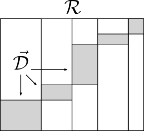
(a) The setting

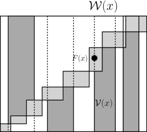
(b) The strategy

            

Figure 6: (a) We have a boxchain $\vec{{\cal D}}$ compatible with strip decomposition $\vec{{\cal S}}$, spanning box ${\cal R}$. (b) We bound $\chi^{out}$ through the dark gray regions. These disjoint regions are constructed through a set of strips. ${\cal V}(x)$ consists of violations in the strip that are not contained in the main box chain.

The set up for the lemma is:

D1

${\cal R}$ is a box.

D2

$\vec{{\cal S}}$ is a strip decomposition of ${\cal R}$, i.e., a partition of ${\cal R}$ into ${\cal R}$-strips.

D3

For $x\in X({\cal R})$, $s(x)$ is the width of the strip containing $x$.

D4

$\mu\in(0,1)$.

D5

An index $x\in X({\cal R})$ is called safe or unsafe, depending on whether it is a $(\mu,s(x))$-safe splitter for ${\cal R}$.

D6

$\vec{{\cal D}}$ is an arbitrary box-chain that is compatible with $\vec{{\cal S}}$. (This means that $\vec{{\cal S}}$ consists of the strips ${\cal D}|{\cal R}$ for ${\cal D}\in\vec{{\cal D}}$. Refer to [fig:dichot1]Fig. 6a.)

D7

An index $x$ such that $F(x)\in\vec{{\cal D}}^{\cup}$ is called a $\vec{{\cal D}}$-index.

D8

$S$ is the set of $\vec{{\cal D}}$-indices $x$ that are safe, and $U$ is the set of $\vec{{\cal D}}$-indices that are unsafe.

D9

$\chi=|{\cal R}\cap{\cal F}|$ is the number of ${\cal F}$-points in ${\cal R}$, $\chi^{in}$ is the number of such points that lie inside ${\cal D}^{\cup}$ and $\chi^{out}=\chi-\chi^{in}$ is the number of such points that lie outside of ${\cal D}^{\cup}$.

Lemma 5.7.

Under hypotheses D1-D9, we have $\chi^{out}\geq\frac{\mu}{1-\mu}|U|$ and $\chi^{in}\leq(1-\mu)\chi+\mu(|S|)$.

The point of the lemma is that if there are few safe indices then the fraction of ${\cal F}$-points of ${\cal R}$ that lie in $\vec{{\cal D}}$ can’t be much larger than $1-\mu$. The idea of the proof is that each unsafe index in $\vec{{\cal D}}^{\cup}\cap{\cal F}$ can be associated to a non-trivial set of points in ${\cal F}$ that are outside of $\vec{{\cal D}}$.

Proof 5.8.

For each $x\in U$, there exists a strip ${\cal W}(x)$ with $x$ on either the left or right end such that ${\cal W}(x)$ is $(\mu,s(x))$-rejecting for $x$. In [fig:dichot2]Fig. 6b, we show such a point $F(x)$ with ${\cal W}(x)$ to the right. Let ${\cal V}(x)$ be the set of violations with $F(x)$, contained in ${\cal W}(x)$ but not in $\vec{{\cal D}}^{\cup}$. In other words, ${\cal V}(x)=\{F(y)|F(y)\not\sim F(x),F(y)\in{\cal W}(x)\setminus\vec{{\cal D}}^{\cup}\}$. In [fig:dichot2]Fig. 6b, the corresponding region in ${\cal W}(x)$ is marked in dark gray. Observe that it is contained in $\vec{{\cal D}}^{SE}$. We now lower bound $|{\cal V}(x)|$.

Claim 6.

$|{\cal V}(x)|\geq\frac{\mu}{1-\mu}|\vec{{\cal D}}^{\cup}\cap{\cal W}(x)\cap{\cal F}|$.

Proof 5.9.

The number of violations with $x$ in ${\cal W}(x)$ is at least $\mu|{\cal F}\cap{\cal W}(x)|+s(x)$. Any violation with $x$ contained in $\vec{{\cal D}}^{\cup}$ must be contained in $\vec{{\cal D}}[x]$ (the unique box of $\vec{{\cal D}}$ whose index set includes $x$). This is because $\vec{{\cal D}}$ is a box chain (a look at [fig:dichot2]Fig. 6b should make this clear). Hence, the number of such violations is at most $0pt(\vec{{\cal D}}[x])\leq s(x)$. Combining, $|{\cal V}(x)|\geq\mu|{\cal F}\cap{\cal W}(x)|$. Since ${\cal V}(x)$ is disjoint with $\vec{{\cal D}}^{\cup}$, $|\vec{{\cal D}}^{\cup}\cap{\cal W}(x)\cap{\cal F}|\leq(1-\mu)|{\cal F}\cap{\cal W}(x)|$ and $|{\cal V}(x)|\geq\frac{\mu}{1-\mu}|\vec{{\cal D}}^{\cup}\cap{\cal W}(x)\cap{\cal F}|$.

Let $L$ (resp. $R$) be the indices $x\in U$ such that $x$ lies to the left (resp. right) of ${\cal W}(x)$. For $x\in R$, ${\cal V}(x)\subseteq\vec{{\cal D}}^{NW}$ (refer to [fig:dichot2]Fig. 6b). Similarly for $x\in L$, ${\cal V}(x)\subseteq\vec{{\cal D}}^{SE}$.

We construct $L^{\prime}\subseteq L$ and $R^{\prime}\subseteq R$ such that:

• The family $\{{\cal W}(x):x\in L^{\prime}\}$ of strips is pairwise disjoint and the family $\{{\cal W}(x):x\in R^{\prime}\}$ is pairwise disjoint.

• $\bigcup_{z\in L^{\prime}}{\cal W}(z)$ contains $\{F(z)|z\in L\}$ and $\bigcup_{z\in R^{\prime}}{\cal W}(z)$ contains $\{F(z)|z\in R\}$.

The sets $L^{\prime}$ and $R^{\prime}$ are constructed separately by simple greedy algorithms. To construct $L^{\prime}$ (resp. $R^{\prime}$), start with $L^{\prime}$ (resp. $R^{\prime}$) set to the $\emptyset$ and repeatedly select the least index $x\in L$ (resp. largest index $x\in R$) for which $F(x)$ is not already covered by ${\cal W}(z)$ for a previously selected $z$.

Let us define ${\cal W}^{\prime}$ to be the union $\bigcup_{x\in L^{\prime}\cup R^{\prime}}{\cal W}(x)$. We lower bound $\chi^{out}$ by $|\bigcup_{x\in L^{\prime}\cup R^{\prime}}{\cal V}(x)|$ which is equal to $|\bigcup_{x\in L^{\prime}}|{\cal V}(x)|+|\bigcup_{x\in R^{\prime}}|$, since ${\cal V}(x)\subseteq\vec{{\cal D}}^{NW}$ for $x\in R$ and ${\cal V}(x)\subseteq\vec{{\cal D}}^{SE}$ for $x\in L$. Furthermore, since ${\cal W}(x)$ are disjoint for $x\in R^{\prime}$ and for $x\in L^{\prime}$, this is equal to $\sum_{x\in L^{\prime}\cup R^{\prime}}|{\cal V}(x)|$. Using [clm:cV]Claim 6 and the fact that $U\subseteq\vec{{\cal D}}^{\cup}\cap{\cal W}^{\prime}$, we obtain:

$$\chi^{out}\geq\Big{|}\bigcup_{x\in L^{\prime}\cup R^{\prime}}{\cal V}(x)\Big{|} = \sum_{x\in L^{\prime}\cup R^{\prime}}|{\cal V}(x)|$$

$$\geq \sum_{x\in L^{\prime}\cup R^{\prime}}\frac{\mu}{1-\mu}|\vec{{\cal D}}^{\cup}\cap{\cal W}(x)\cap{\cal F}|$$

$$\geq \frac{\mu}{1-\mu}|\vec{{\cal D}}^{\cup}\cap{\cal W}^{\prime}(x)|\geq\frac{\mu}{1-\mu}|U|.$$

For the second conclusion of the lemma, using $\chi^{in}=|U|+|S|$ we get:

$$\chi^{in}=\chi-\chi^{out} \geq \chi-\frac{\mu}{1-\mu}|U|$$

$$= \chi-\frac{\mu}{1-\mu}(\chi^{in}-|S|).$$

Multiplying both sides by $1-\mu$ and adding $\mu\chi^{in}$ to both sides yields the desired inequality. ∎

5.5 Value nets and the subroutine BuildNet

Given a box, we want to select a suitably representative set of values from the box. Let us say that a value interval $J$ is $\alpha$-popular for box ${\cal B}$ if there are at least $\alpha 0pt({\cal B})$ indices $x\in X({\cal B})$ such that $f(x)\in J$. If ${\cal B}$ is a box and $\alpha\in(0,1)$, a $\alpha$-value net for ${\cal B}$ is a subset $V$ of $Y({\cal B})$ such that:

• $y_{T}({\cal B})\in V$.

• For all subintervals $J$ of $Y({\cal B})$ that are $\alpha$-popular for ${\cal B}$, $V\cap J\neq\emptyset$.

Refer to [fig:valuenet]Fig. 7a. The value net contains a value in $J$ whenever the corresponding dark gray region contains at least $\alpha 0pt({\cal B})$ ${\cal F}$-points.

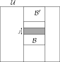
(a) Value nets

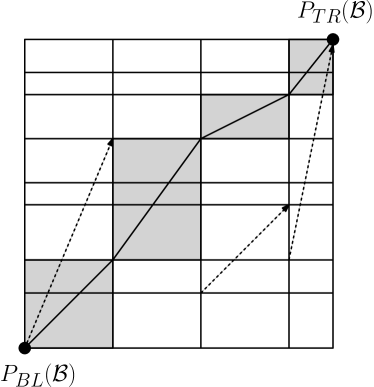
(b) The digraph $D(\Gamma)$

            

Figure 7: (a) If the number of points in the gray region is large enough, then a value net must contain a value in $J$. (b) All grid points (which are internal to the box) are vertices. The dashed arrows show the 3 different types of arcs in $D(\Gamma)$. The solid line traces a $D(\Gamma)$ path, and the corresponding box chain is colored gray.

If we had access to the set of values $Y({\cal B})\cap f(X({\cal B}))$ in nondecreasing order, then we could construct a $\alpha$-value net for ${\cal B}$ by taking those values whose position in the order is a multiple of $\lceil\alpha 0pt({\cal B})\rceil$. However, we can only access the values indirectly by evaluating $f$ at indices in $X({\cal B})$ so constructing this order would require evaluating $f$ at every index in $X({\cal B})$, which is too time consuing.

To construct a $\alpha$-value net quickly we use random sampling.

Proposition 7.

There is a randomized procedure ${\rm{\bf BuildNet}}$ that takes as input a triple $({\cal B},\alpha,\xi)$ where ${\cal B}$ is a box and $\alpha,\xi\in(0,1)$, runs in time $(1/\alpha)^{O(1)}\log(1/\xi)$ and outputs a subset $V$ of $Y({\cal B})$ of size at most $4\lceil 1/\alpha\rceil$ such that with probability at least $1-\xi$, $V$ is a $\alpha$-value net for ${\cal B}$.

Proof 5.10.

Given a box ${\cal B}$, let ${\cal B}^{\prime}$ be the strip ${\cal B}|{\cal U}$. (This is the set of all points whose index belongs to $X({\cal B})$.) It suffices to construct a $\alpha$-value net $V^{\prime}$ for ${\cal B}^{\prime}$. Once we do this we take $V=V^{\prime}\cap Y({\cal B})\cup\{y_{T}({\cal B})\}$. This is a $\alpha$-value net for ${\cal B}$ since every $\alpha$-popular value interval $J$ for ${\cal B}$ is also $\alpha$-popular for ${\cal B}^{\prime}$.

So let us construct a $\alpha$-value net for ${\cal B}^{\prime}$. Let $s=4\lceil 1/\alpha\rceil$. Let $M=\lceil s\ln(s/2\xi)\rceil$. Let $R$ be a sequence of $sM-1$ uniform random samples from $X({\cal B}^{\prime})$ and let $y_{1}\leq\cdots\leq y_{sM-1}$ be their $y$-values in sorted order. Note that all of these are in $Y({\cal B}^{\prime})$. Let $y_{0}=0$ and $y_{sM}={\tt valbound}$. Define $V=\{y_{iM}:i\in[1,s-1]\}$.

We analyze the probability that $V$ is not a $\alpha$-value net for ${\cal B}^{\prime}$.

Let $B=\lceil\alpha 0pt({\cal B}^{\prime})/2\rceil$ (which is also equal to $\lceil\alpha 0pt({\cal B})/2\rceil$). Let $x_{1},\ldots,x_{0pt({\cal B})}$ be the indices of $X({\cal B}^{\prime})$ ordered so that $f(x_{1})\leq\cdots\leq f(x_{0pt({\cal B}^{\prime})})$. Write $0pt({\cal B}^{\prime})$ as $qB+r$ where $r<B$, and note that $q\leq 0pt({\cal B}^{\prime})/B\leq 2/\alpha\leq s/2$. Partition $x_{1},\ldots,x_{qB}$ into $q$ “bins”, where each bin is a sequence of $B$ consecutive indices. Let $A_{i}$ for $i\in[1,q]$ be the number of samples from $R$ that fall in bin $i$.

We now show that (1) with probability at least $1-\xi$, $A_{i}\geq M$ for all $i\in[1,q]$, and (2) if $A_{i}\geq M$ for each $i$, then $V$ is a $\alpha$-value net for ${\cal B}^{\prime}$.

We prove (2) first. Note that $V$ contains at least $1$ value from each bin. Let $J$ be a $\alpha$-popular subinterval of $Y({\cal B}^{\prime})$. Then $|F^{-1}(J)\cap X({\cal B}^{\prime})|\geq\alpha 0pt({\cal B}^{\prime})>2B-2$. Since $F^{-1}(J)\cap X({\cal B}^{\prime})$ is a consecutive subsequence of $x_{1},\ldots,x_{0pt({\cal B}^{\prime})}$, it must contain at least one bin, and hence intersects $V$.

It remains to prove (1). Fix $i\in[1,q]$ and consider the event that $A_{i}\leq M-1$. $A_{i}$ is the sum of $sM-1$ Bernoulli trials each having probability at least $\frac{B}{0pt({\cal B}^{\prime})}\geq\alpha/2$, and so has expectation at least $\frac{\alpha}{2}(sM-1)\geq 2M-1$. By [prop:hoeff1]Prop. 1, . By the union bound, the probability that some $A_{i}\leq M-1$ is at most $se^{-M/s}/2$ and by the choice of $M$ this is at most $\xi$. This completes the proof of the value net construction for ${\cal B}^{\prime}$.

5.6 Grids, the subroutine BuildGridand grid digraphs

A grid $\Gamma$ is a ${\cal B}$-grid if $X(\Gamma)\subset X({\cal B})-\{x_{L}({\cal B}),x_{R}({\cal B})\}$ and $Y({\cal B})$ is a value net for ${\cal B}$. If $x_{1}<\cdots<x_{k}$ are the indices of $X(\Gamma)$, then they define a ${\cal B}$-strip decomposition of $X({\cal B})$ whose associated index partition is $(x_{L}({\cal B}),x_{1}],(x_{1},x_{2}],\cdots,(x_{k},x_{R}({\cal B})]$. We call this the strip decomposition of ${\cal B}$ induced by $\Gamma$.

Definition 5.11.

For a box ${\cal B}$ and $\alpha>0$, a grid $\Gamma$ is an $\alpha$-fine ${\cal B}$-grid if:

• $X(\Gamma)$ contains an index from every subinterval $I$ of $X({\cal B})$ having size exceeding $\alpha 0pt({\cal B})$.

• $Y(\Gamma)$ is a $\frac{\alpha}{|X(\Gamma)|}$-value net.

We define a procedure ${\rm{\bf BuildGrid}}{}$ that takes as input a triple $({\cal B},\alpha,\xi)$ (as does BuildNet) and outputs a ${\cal B}$-grid $\Gamma$ that is $\alpha$-fine with probability at least $1-\xi$.

The procedure works as follows. If $0pt({\cal B})\leq 1/\alpha$ then $X(\Gamma)=X({\cal B})$ and $Y(\Gamma)=Y({\cal B})$. Otherwise, set $r=\lceil 1/\alpha\rceil$ and for $i\in[0,r]$, define $x_{i}=x_{L}({\cal B})+\lfloor i\alpha 0pt({\cal B})\rfloor$. We take $X(\Gamma)=\{x_{1},\ldots,x_{r-1}\}$. It follows that $x_{0}=x_{L}({\cal B})$, $x_{r}=x_{R}({\cal B})$ and $x_{i}-x_{i-1}\leq\lceil\alpha 0pt({\cal B})\rceil$ for each $i\in[1,r]$. The set $Y(\Gamma)$ is constructed by applying ${\rm{\bf BuildNet}}({\cal B},\alpha^{2}/2,\xi)$. We say that ${\rm{\bf BuildGrid}}({\cal B},\alpha,\xi)$ is reliable if the grid $\Gamma$ that it outputs is $\alpha$-fine. The definition of the grid, together with [prop:buildnet]Prop. 7 implies:

Proposition 9.

${\rm{\bf BuildGrid}}({\cal B},\alpha,\xi)$ produces a grid $\Gamma$ with $|X(\Gamma)|\leq 1+\lceil 1/\alpha\rceil\leq 3/\alpha$ and $|Y(\Gamma)\leq\lceil 8/\alpha^{2}\rceil\leq 16/\alpha^{2}$ that is reliable with probability at least $1-\xi$.

Grid digraph $D(\Gamma)$: This is associated with the ${\cal B}$-grid $\Gamma$. The vertex set is $\Gamma\cup\{P_{BL}({\cal B}),P_{TR}({\cal B})\}$. The arc sets consists of pairs $(P_{BL}({\cal B}),Q)$ where $Q$ lies in the leftmost columnn of $\Gamma$, $(Q,P_{TR}({\cal B}))$ where $Q$ belongs to the rightmost column of $\Gamma$, and $(P,Q)$ where $P\prec Q$ and $P$ and $Q$ are in adjacent columns of $\Gamma$. $D(\Gamma)$ is acyclic and has unique source $P_{BL}({\cal B})$ and unique sink $P_{TR}({\cal B})$. A $D(\Gamma)$-path is a source-to-sink path in $D(\Gamma)$. Every arc $(P,Q)$ of $D(\Gamma)$ corresponds to a box $Box(P,Q)$ and a $D(\Gamma)$-path corresponds to a ${\cal B}$-box chain. A box chain arising in this way is a $D(\Gamma)$-chain. Each box correponding to an arc is called a grid box. Refer to [fig:digraph]Fig. 7b.

The following lemma says that if $\Gamma$ is a $\alpha$-fine ${\cal B}$-grid then for any increasing sequence in ${\cal B}$ there is a $D(\Gamma)$-chain that contains all but a small number of points from the sequence.

Lemma 5.12.

(Grid approximation lemma) Suppose $\Gamma$ is a $\alpha$-fine ${\cal B}$-grid. Let ${\cal L}$ be an increasing sequence of ${\cal F}$-points in ${\cal B}$. Then there is a $D(\Gamma)$-chain $\vec{{\cal D}}=({\cal D}_{1},\dots,{\cal D}_{r})$ such that the subset ${\cal L}-\vec{{\cal D}}^{\cup}$ has size at most $\alpha 0pt({\cal B})$.

Proof 5.13.

Let $X(\Gamma)=\{x_{1}<\ldots<x_{r}\}$. To specify a $D(\Gamma)$-chain we need to choose a nondecreasing comparable sequence of points $P_{1},\ldots,P_{r}$, such that $P_{i}$ is in column $x_{i}$ of $\Gamma$. Let ${\cal L}_{i}$ be the portion of ${\cal L}$ with $x$ coordinate at most $x_{i}$ and let $Q_{i}$ be the largest point in ${\cal L}_{i}$. Take $P_{i}$ to be the least point of $\Gamma$ in column $i$ such that $Q_{i}\preceq P_{i}$.

The points of ${\cal L}$ that lie outside of the corresponding box chain are those that belong to $P_{i}^{NW}$ or $P_{i}^{SE}$ for some point $P_{i}$. Since every point of ${\cal L}_{i}$ is less than $P_{i}$, there are no points of ${\cal L}$ in $P_{i}^{NW}$. The points of ${\cal L}$ in $P_{i}^{SE}$ have $x$-coordinate greater than $x_{i}$ and $y$-coordinate strictly between $y(Q_{i})$ and $y(P_{i})$. By choice of $P_{i}$, there is no value in $Y(\Gamma)$ strictly between $y(Q_{i})$ and $y(P_{i})$. Since $Y(\Gamma)$ is a $\alpha/r$-value net for ${\cal B}$, there are at most $\alpha 0pt({\cal B})/r$ points of ${\cal L}$ in $P_{i}^{SE}$.

Since each point $P_{i}$ is in violation with at most $\alpha 0pt({\cal B})/r$ points of ${\cal L}$, the total number of points of ${\cal L}$ that violate some $P_{i}$ is at most $\alpha 0pt({\cal B})$.

6 The basic LIS approximation algorithm

In this section we describe the algorithm BasicMain, which achieves the properties stated in [thm:alg1]Thm. 4.1. As asserted in the theorem, BasicMain takes as input a natural number $n$, an array $f$ of size $n$ and an error parameter $\overline{\tau}\in(0,1)$ and outputs an estimate to ${\tt lis}_{f}$. Recall that we assume the values of the array are in the range $[1,{\tt valbound}]$, where ${\tt valbound}$ is a known integer.

The program BasicMain sets certain global parameters, initializes a parameter $t_{\max}$ and then calls a subroutine ${\rm{\bf ApproxLIS}}$, which is the main part of the algorithm. The subroutine ${\rm{\bf ApproxLIS}}$ takes as input a box ${\cal B}$ and a nonnegative integer $t$ and outputs an estimate of ${\tt lis}_{f}({\cal B})$. We denote an invocation of ${\rm{\bf ApproxLIS}}$ on box ${\cal B}$ with parameter $t$ by ${\rm{\bf ApproxLIS}}_{t}({\cal B})$. The global parameters are all used within ${\rm{\bf ApproxLIS}}$ and the procedures it calls. The values for the global parameters are chosen to make the error analysis work. The array size $n$ and the array $f$ are also treated as global parameters in ${\rm{\bf ApproxLIS}}$.

${\rm{\bf BasicMain}}(n,f,\overline{\tau})$ Output: Approximation to ${\tt lis}_{f}$. 1. Fix global parameters according to table (unchanged throughout algorithm). Name Symbol Value Initial precision $t_{\max}$ $\lceil 4/\overline{\tau}\rceil$ Sample size parameter $\sigma$ $10(\log n)^{4}$ Grid precision parameter $\alpha$ $\gamma$ Width threshold $\omega$ $1/\rho$ Tainting parameter $\eta$ $\frac{1}{10\log n}$ Primary splitter parameter $\mu_{r}$ $2/(r+3)$ Secondary splitter parameter $\gamma$ $\frac{1}{(C_{1}\log n)^{3}}$ Splitter balance parameter $\rho$ $\frac{1}{C_{1}\log n}$ 2. Let box ${\cal U}$ be the box $[1,n]\times[1,{\tt valbound}]$. 3. Return ${\rm{\bf ApproxLIS}}_{t_{\max}}({\cal U})$.

The algorithm ${\rm{\bf ApproxLIS}}$ is recursive, and in recursive calls will be run on r values of $t\leq t_{\max}$ and subboxes ${\cal B}$ of ${\cal U}$. We will prove the following property of ${\rm{\bf ApproxLIS}}$:

Theorem 6.1.

Suppose ${\rm{\bf ApproxLIS}}$ is run with the global parameters set as in ${\rm{\bf BasicMain}}$. On input a box ${\cal B}\subseteq{\cal U}$ and an integer $t$, ${\rm{\bf ApproxLIS}}_{t}({\cal B})$:

• runs in time $(\log n)^{O(t)}$, and

• outputs a value that, with probability at least $1-n^{-\Omega(\log(n)}$, is a $(\tau_{t},\delta_{t})$-approximation to ${\tt lis}({\cal B})$, where:

  $$\tau_{t} = \frac{4}{t}$$

  $$\delta_{t} = \frac{t}{\log(n)}.$$

[thm:alg1]Thm. 4.1 follows immediately from [thm:basic approxlis]Thm. 6.1:

Proof 6.2 (of [thm:alg1]Thm. 4.1).

${\rm{\bf BasicMain}}(n,f,\overline{\tau})$ returns the output of ${\rm{\bf ApproxLIS}}_{t_{\max}}({\cal U})$. By [thm:basic approxlis]Thm. 6.1, this gives a $(4/t_{\max},t_{\max}/\log(n))$-approximation to ${\tt lis}_{f}$ which runs in time $\log(n)^{O(t_{\max})}$. Using the fact that $t_{\max}=\lceil 4/\overline{\tau}\rceil$ which is between $4/\overline{\tau}$ and $5/\overline{\tau}$ gives the desired running time and approximation error for ${\rm{\bf BasicMain}}$.

6.1 Description and pseudocode for ApproxLIS

The procedure ${\rm{\bf ApproxLIS}}$, uses four subprocedures ${\rm{\bf Classify}}$, ${\rm{\bf CriticalBox}}$, ${\rm{\bf TerminalBox}}$, and ${\rm{\bf GridChain}}$, each taking as input a box ${\cal B}$ and a nonnegative quality parameter $t$, and possibly other input. These procedures use the previously defined procedures ${\rm{\bf FindSplitter}}$ and ${\rm{\bf BuildGrid}}$. For later convenience, we put the quality parameter as a subscript to the procedure.

The main approximation algorithm ${\rm{\bf ApproxLIS}}_{t}({\cal B})$ returns an estimate of ${\tt lis}({\cal B})$. If the input box ${\cal B}$ has width 1, then it outputs $|{\cal F}\cap{\cal B}|$. Otherwise, ${\rm{\bf ApproxLIS}}_{t}$ uses a subroutine ${\rm{\bf Classify}}_{t}$. This takes as input ${\cal B}$ and an index $x\in X({\cal B})$ and outputs a classification of $x$ as good or bad. ${\rm{\bf ApproxLIS}}_{t}({\cal B})$ outputs an estimate of the number of good point by running ${\rm{\bf Classify}}_{t}(x,{\cal B})$ on a small random sample of indices.

Recall from Section 5.1 that our viewpoint of fixing the random bits at the outset specifies the behavior of ${\rm{\bf Classify}}_{t}$ on every index. We define $Good_{t}({\cal B})$ to be the set of indices $x$ for which ${\rm{\bf Classify}}_{t}(x,{\cal B})$ would return good. Thus ${\rm{\bf ApproxLIS}}_{t}({\cal B})$ returns an estimate of $|Good_{t}({\cal B})|$. The algorithm ${\rm{\bf Classify}}_{t}$ is designed so that $Good_{t}({\cal B})$ is the index set of an increasing sequence, and with probability close to 1, is close in size to ${\tt lis}({\cal B})$. Hence, ${\rm{\bf ApproxLIS}}_{t}({\cal B})$ should be a good estimate of ${\tt lis}({\cal B})$.

The procedure ${\rm{\bf Classify}}_{t}$ is recursive. If $F(x)\not\in{\cal B}$, then $x$ is declared bad. Otherwise, if ${\cal B}$ has width 1, we declare $x$ to be good, and if $0pt({\cal B})>1$ and $t=0$ then $x$ is declared bad. The main case ($F(x)\in{\cal B}$, $0pt({\cal B})>1$ and $t\geq 1$) is accomplished by calling ${\rm{\bf CriticalBox}}_{t}(x,{\cal B})$, which returns a subbox ${\cal C}$ of ${\cal B}$ such that $x\in X({\cal C})$. The procedure then recursively calls ${\rm{\bf Classify}}_{t-1}(x,{\cal C})$. The classification returned by this recursive call is the output of ${\rm{\bf Classify}}_{t}(x,{\cal B})$.

The procedure ${\rm{\bf CriticalBox}}_{t}(x,{\cal B})$ finds a subbox ${\cal C}$, called the critical subbox of ${\cal B}$ for $x$. The procedure operates in two stages. The first stage is performed by ${\rm{\bf TerminalBox}}$, which shrinks ${\cal B}$ to a subbox ${\cal T}$, called the terminal box with $x\in X({\cal T})$. Intuitively, ${\rm{\bf TerminalBox}}$ attempts to simulate the interactive protocol discussed in the introduction. ${\rm{\bf TerminalBox}}({\cal B},x)$ initializes ${\cal T}$ to ${\cal B}$. It uses the subroutine ${\rm{\bf FindSplitter}}{}$ to look for an index $s$ such that $F(s)\in{\cal T}$ and $s$ is a good splitter for the ${\cal B}$-strip ${\cal T}|{\cal B}$. If ${\rm{\bf FindSplitter}}$ succeeds in finding $s$, then the splitter defines a box chain of size 2 spanning ${\cal T}$, and ${\cal T}$ is replaced by the box in the chain whose index set contains $x$. This process is repeated until either $0pt({\cal T})\leq\omega$ (${\cal T}$ is narrow) or ${\rm{\bf FindSplitter}}$ fails to find a good splitter. This ends the first stage.

In the second stage, a box chain $\vec{{\cal C}}({\cal T})$ spanning ${\cal T}$, called the critical chain for ${\cal T}$, is constructed. Intuitively, this part implements approximation boosting sketched in the introduction. We use ${\rm{\bf BuildGrid}}$ to build a suitably fine grid for ${\cal T}$ of size $(\log n)^{O(1)}$. We then recursively evaluate ${\rm{\bf ApproxLIS}}_{t-1}({\cal C})$ for every grid box ${\cal C}$. Think of these values as giving a length function on the edges of the grid digraph. The procedure performs a longest path computation to compute the exact longest path in the grid digraph from the lower left corner to the upper right corner of ${\cal T}$. (This computation takes $(\log n)^{O(1)}$ time.)

Having found the critical chain $\vec{{\cal C}}({\cal T})$, the output of ${\rm{\bf CriticalBox}}$ is the box $\vec{{\cal C}}({\cal T})[x]$ of $\vec{{\cal C}}({\cal T})$ whose index set contains $x$.

The pseudocode for the algorithm is presented below. The arguments ${\cal B},{\cal T}$ represent boxes, $t$ is a nonnegative integer, and $x$ is an index. The array $f$ and the domain size $n$ are treated as implicit global parameters.

${\rm{\bf ApproxLIS}}_{t}({\cal B})$ Output: Approximation to ${\tt lis}({\cal B})$. 1. If $0pt({\cal B})=1$, output $|{\cal B}\cap{\cal F}|$. 2. Otherwise ($0pt({\cal B})>1$): Select $\sigma$ uniform random indices from $X({\cal B})$. Run ${\rm{\bf Classify}}_{t}(x,{\cal B})$ on each sample point. Let $g$ be the number of points classified as $good$ and return $g0pt({\cal B})/\sigma$.

${\rm{\bf Classify}}_{t}(x,{\cal B})$ Output: good or bad 1. If $F(x)\not\in{\cal B}$, return bad. 2. Otherwise ($F(x)\in{\cal B}$) (a) Base case: If $0pt({\cal B})=1$, return good. If $t=0$ and $0pt({\cal B})>1$, return bad. (b) Main case ($0pt({\cal B})>1$ and $t\geq 1$): i. ${\cal C}\longleftarrow{\rm{\bf CriticalBox}}_{t}(x,{\cal B})$. ii. Run ${\rm{\bf Classify}}_{t-1}(x,{\cal C})$ and return its output.

${\rm{\bf CriticalBox}}_{t}(x,{\cal B})$ Output: Subbox ${\cal C}$ of ${\cal B}$ such that $x\in X({\cal C})$ 1. ${\cal T}\longleftarrow{\rm{\bf TerminalBox}}_{t}(x,{\cal B})$. 2. Call ${\rm{\bf GridChain}}_{t}({\cal T})$ and let $\vec{{\cal C}}({\cal T})$ be the chain of boxes returned. 3. Return $\vec{{\cal C}}({\cal T})[x]$ (the box ${\cal C}\in\vec{{\cal C}}({\cal T})$ with $x\in X({\cal C})$).

${\rm{\bf TerminalBox}}_{t}(x,{\cal B})$ Output: subbox ${\cal T}$ of ${\cal B}$ such that $x\in X({\cal T})$. 1. Initialize ${\cal T}$ to ${\cal B}$ and boolean variable $splitter\_found$ to TRUE. 2. Repeat until $0pt({\cal T})\leq\omega$ (${\cal T}$ is narrow) or $splitter\_found$ is FALSE: (a) Run ${\rm{\bf FindSplitter}}({\cal T},{\cal B},\mu_{t},\gamma 0pt({\cal T}),\rho)$: returns boolean $splitter\_found$ and index $splitter$. (b) If $splitter\_found={\tt TRUE}$ then i. If $x\leq splitter$ then replace ${\cal T}$ by the box $Box(P_{BL}({\cal T}),F(splitter))$. ii. If $x>splitter$ then replace ${\cal T}$ by the box $Box(F(splitter),P_{TR}({\cal T}))$. 3. Return ${\cal T}$.

${\rm{\bf GridChain}}_{t}({\cal T},\alpha)$ Output: box chain $\vec{{\cal C}}({\cal T})$ spanning ${\cal T}$. 1. Call ${\rm{\bf BuildGrid}}({\cal T},\alpha,n^{-2\log n})$ which returns a grid $\Gamma$. 2. Construct the associated digraph $D(\Gamma)$ 3. For each grid-box ${\cal D}$ of $D(\Gamma)$. recursively evaluate ${\rm{\bf ApproxLIS}}_{t-1}({\cal D})$. 4. Compute the longest path in $D(\Gamma)$ from $P_{BL}({\cal T})$ to $P_{TR}({\cal T})$ according to the length function ${\rm{\bf ApproxLIS}}_{t-1}({\cal D})$. 5. Return the $\Gamma$-chain $\vec{{\cal C}}({\cal T})$ associated to the longest path.

7 Properties of ApproxLIS

In this section and the next we prove [thm:basic approxlis]Thm. 6.1 by showing that a call to ${\rm{\bf ApproxLIS}}_{t}({\cal B})$ runs in time $(\log n)^{O(t)}$ and that with probability $1-n^{O((\log n)}$. the output is within $\tau_{t}{\tt loss}({\cal B})+\delta_{t}0pt({\cal B})$ of ${\tt lis}({\cal B})$.

We first present the easy running time analysis. We next turn to the much more difficult task of bounding the error of the estimate returned by the algorithm. We start with some important structural observations about the behavior of the algorithm. We then identify two assumptions about the random bits used by the algorithm, which encapsulate all that we require from the random bits in the error analysis. We show that these assumptions hold with probability very close to 1.

In [sec:correctness]§8 we formulate and prove [thm:basic correctness]Thm. 8.1, which says that whenever the two assumptions hold then ${\rm{\bf ApproxLIS}}$ returns a suitably accurate estimate, and which immediately implies the desired error bounds in Theorem 6.1.

7.1 Running time analysis

Let $A_{t}=A_{t}(n)$ be the running time of ${\rm{\bf ApproxLIS}}_{t}$ and $C_{t}=C_{t}(n)$ be the running time of ${\rm{\bf Classify}}_{t}$ on boxes of width at most $n$. In what follows we use $P_{i}=P_{i}(n)$ to denote functions of the form $a_{i}((\log n))^{b_{i}}$, where $a_{i},b_{i}$ are constants that are independent of $n$ and $t$.

Claim 10.

For all $t\geq 1$,

$$A_{t} \leq P_{1}C_{t}+P_{2}.$$

$$C_{t} \leq C_{t-1}+P_{3}A_{t-1}+P_{4}.$$

Proof 7.1.

The first recurrence with $P_{1}=\sigma=10(\log n)^{4}$ is immediate from the definition of ${\rm{\bf ApproxLIS}}_{t}$. The function $P_{2}$ is an upper bound on the cost of operations within ${\rm{\bf ApproxLIS}}_{t}$ excluding the calls to ${\rm{\bf Classify}}_{t}$

For the second recurrence, the final recursive call to ${\rm{\bf Classify}}_{t-1}$ gives the $C_{t-1}$ term. The rest of the cost comes from ${\rm{\bf CriticalBox}}_{t}$ which invokes ${\rm{\bf TerminalBox}}_{t}$, which involves several iterations whose cost is dominated by the cost of ${\rm{\bf FindSplitter}}$. Each iteration reduces the width of ${\cal T}$ by at least a $(1-\rho)$ factor, so the number of iterations is at most $(\log n)/\rho$. The cost of ${\rm{\bf FindSplitter}}$ is $(\log n)^{O(1)}$, so the cost of ${\rm{\bf TerminalBox}}_{t}$ is included in the term $P_{4}$. ${\rm{\bf CriticalBox}}_{t}$ then calls ${\rm{\bf GridChain}}_{t}$. This involves building a grid of size $(\log n)^{O(1)}$ and making one call to ${\rm{\bf ApproxLIS}}_{t}$ for each grid box, which accounts for the term $P_{3}A_{t-1}$. All of the rest of the cost of ${\rm{\bf GridChain}}_{t}$ is in doing a longest path computation on the grid digraph, which is absorbed into the $P_{4}$ term.

Corollary 7.2.

For all $t\geq 1$, $A_{t}$ and $C_{t}$ are in $\log n^{O(t)}$.

Proof 7.3.

Note that $A_{0},C_{0}=(\log n)^{O(1)}$. By the recurrences of [clm:runtime]Claim 10, $C_{t}\leq P_{5}(P_{1}P_{3}+1)^{t}$ and $A_{t}\leq P_{6}(P_{1}P_{3}+1)^{t}$ which are both $(\log n)^{O(t)}$.

7.2 The t-splitter tree and terminal chain

We analyze the structure of the output of ${\rm{\bf TerminalBox}}_{t}$. This procedure takes three parameters: the level $t$, the box ${\cal B}$ and an index $x$. It also uses randomness within the calls to ${\rm{\bf FindSplitter}}$. Recall from Section 5.1 that we classify the random bits used in ${\rm{\bf ApproxLIS}}$ as primary random bits and all other random bits as secondary. Since ${\rm{\bf TerminalBox}}_{t}$ never calls ${\rm{\bf ApproxLIS}}$, all random bits used are secondary.

In the following discussion, the box ${\cal B}$, level $t$, and secondary random bits as fixed. Under this view, ${\rm{\bf TerminalBox}}$ maps each index $x\in X({\cal B})$ to a box ${\cal T}(x)$. We now define the $t$-splitter tree, which summarizes all important information about the execution and output of ${\rm{\bf TerminalBox}}_{t}(x,{\cal B})$.

For each subbox ${\cal T}$ of ${\cal B}$, consider the output of ${\rm{\bf FindSplitter}}_{t}({\cal T},{\cal B},\mu_{t},\gamma 0pt({\cal T}),\rho)$. If $splitter\_found$ is FALSE we say that ${\cal T}$ is splitterless. Otherwise, we say that ${\cal T}$ is split. For each split box ${\cal T}$, ${\rm{\bf FindSplitter}}$ returns a splitter $s=splitter({\cal T})$ which is used to define two subboxes of ${\cal T}$: the left child $Box(P_{BL}({\cal T}),F(s))$ and the right child $Box(F(s),P_{TR}({\cal T}))$. Note that, when viewed as boxes in the plane, the left child lies below and to the left of the right child. The left- and right-child relations together define a directed acyclic graph on the subboxes of ${\cal B}$ in which each splitterless box has out-degree 0 and each split box has out-degree 2. Note that if there is a path from box ${\cal T}$ to box ${\cal T}^{\prime}$ then ${\cal T}^{\prime}\subset{\cal T}$.

Now consider the subdigraph $R({\cal B})$ induced on the set of boxes reachable from ${\cal B}$.

• $R({\cal B})$ is a binary tree rooted at ${\cal B}$. We refer to $R({\cal B})$ as the $t$-splitter tree for ${\cal B}$ and the leaves of the tree as terminal boxes.

• The sequence of boxes encountered along any root-to-leaf path are nested.

• Two boxes ${\cal T}$ and ${\cal T}^{\prime}$ in the tree such that neither is an ancestor of the other have disjoint index sets, i.e. $X({\cal T})\cap X({\cal T}^{\prime})=\emptyset$.

• The terminal boxes together form a box chain that spans ${\cal B}$, called the terminal chain, which we denote by $\vec{{\cal T}}=\vec{{\cal T}}_{t}({\cal B})$.

• Recall (from Section 3.1) that the box chain $\vec{{\cal T}}$ has an associated increasing sequence of points and ${\cal P}^{\circ}(\vec{{\cal T}})$ denotes this sequence, excluding the first and last point. Every point $P\in{\cal P}^{\circ}(\vec{{\cal T})}$ is the splitter of a unique non-terminal box of $R({\cal B})$, denoted ${\cal H}(P)$.

• The point sequence ${\cal P}^{\circ}(\vec{{\cal T}})$ associated to $\vec{{\cal T}}$ is the same as the sequence obtained by doing a depth first traversal of the tree $R({\cal B})$, always visiting the left child of a node before the right child, and recording the sequence of splitters $splitter({\cal H})$ in post-order (listing the splitter of box ${\cal H}$ immediately after having listed all splitters in its left subtree).

• Each terminal box ${\cal T}$ contains a grid $\Gamma({\cal T})$, as formed in the procedure ${\rm{\bf GridChain}}$. We can concatenate grid chains spanning each ${\cal T}\in\vec{{\cal T}}$ to get a box chain that spans ${\cal B}$. This is called a spanning terminal-compatible grid chain in ${\cal B}$. Note that there are many possible such spanning terminal-compatible grid chains.

The following lemma is evident from the above observations and the definition of ${\rm{\bf TerminalBox}}_{t}$:

Lemma 7.4.

For every $x\in F^{-1}({\cal B})$, the set of boxes in the $t$-splitter tree of ${\cal B}$ whose index set contains $x$ is a root-to-leaf path in the tree. This path is equal to the sequence of boxes produced during the execution of ${\rm{\bf TerminalBox}}_{t}(x,{\cal B})$. In particular, the leaf that is reached is the terminal box that is returned by ${\rm{\bf TerminalBox}}_{t}(x,{\cal B})$, and is equal to $\vec{{\cal T}}[x]$ (the unique box ${\cal T}\in\vec{{\cal T}}$ such that $x\in X({\cal T})$).

7.3 Two assumptions about the random bits

As described in Section 5.1, the random bits used in the algorithm are classified as either secondary random bits (those used in ${\rm{\bf FindSplitter}}$ and ${\rm{\bf BuildGrid}}$), and primary randomness used within ${\rm{\bf ApproxLIS}}$. Note that the procedures ${\rm{\bf FindSplitter}}$ and ${\rm{\bf BuildGrid}}$ do not involve calls to themselves or other procedures, while ${\rm{\bf ApproxLIS}}_{t}$ makes calls to ${\rm{\bf Classify}}_{t}$, and ${\rm{\bf Classify}}_{t}$ makes calls to ${\rm{\bf ApproxLIS}}_{t-1}$. The primary random bits used in all calls to ${\rm{\bf ApproxLIS}}_{t}$ for a fixed $t$ are called the level $t$ random bits.

We now identify two assumptions about the random bits used in the algorithm and show that these assumptions hold with probability $1-n^{\Omega(-(\log n))}$. These assumptions encapsulate the only properties of the random bits needed for the error analysis. In the main analysis performed in the next section, we assume that all random bits are fixed so that these conditions are satisfied. The algorithm can then be viewed as deterministic. The first assumption involves the secondary random bits.

Assumption 1. For every possible choice of arguments, the procedures ${\rm{\bf FindSplitter}}$ and ${\rm{\bf BuildGrid}}$ are reliable according to the definitions in Sections 5.3 and 5.6.

Propositions 5 and 9 imply that the probability that a call to ${\rm{\bf FindSplitter}}$ or ${\rm{\bf BuildGrid}}$ is unreliable is $n^{-\Omega((\log n)}$. As indicated earlier, there are at most $n^{O(1)}$ different possible arguments to either procedure, so we can apply a union bound.

Proposition 11.

The probability that Assumption 1 fails is at most $n^{-\Omega(\log(n)}$.

We henceforth view the secondary randomness as fixed in a way that satisfies Assumption 1. We note an important consequence of Assumption 1 that we’ll need later. Recall that for a box ${\cal B}$, with terminal chain $\vec{{\cal T}}$, each point $P\in{\cal P}^{\circ}({\cal T})$ was found as the splitter of a unique non-terminal box ${\cal H}(P)$. Under Assumption 1, and the definition of reliable, each of those splitters is $(\mu_{t},2\gamma w({\cal H}(P)))$-safe for ${\cal H}(P)$.

Proposition 12.

Under assumption 1, for any box ${\cal B}$ with terminal chain $\vec{{\cal T}}$, each of the points $P\in{\cal P}^{\circ}({\cal T})$ is $(\mu_{t},2\gamma w({\cal H}(P)))$-safe for th box ${\cal H}(P)$.

Next we turn to the second assumption. Assumption 2 will state the conditions we need for the primary randomness. To formulate this assumption, we now introduce a somewhat technical definition of tainted boxes. We do not need this definition to analyze the basic ${\rm{\bf ApproxLIS}}$ algorithm, but the improved version will need this notion. We introduce this notion here because this will allow us to reuse the proof for the improved algorithm.

For any $x\in{\cal B}$ and integer $t$, the output of ${\rm{\bf Classify}}_{t}(x,{\cal B})$ is either good or bad. The set of indices classified good is denoted by $Good_{t}({\cal B})$. The procedure ${\rm{\bf ApproxLIS}}_{t}$ tries to approximate $|Good_{t}({\cal B})|$ by random sampling. The randomness used for this random sampling is primary randomness from level $t$. is therefore independent of $Good_{t}({\cal B})$.

Definition 7.5.

Let $\eta$ be the taint parameter specified within BasicMain. A box-level pair $({\cal B},t)$ is said to be tainted if $t\geq 1$ and $0pt({\cal B})>1$ and at least one of the following holds:

• $|{\rm{\bf ApproxLIS}}_{t}({\cal B})-|Good_{t}({\cal B})||>\eta 0pt({\cal B})$.

• There exists a spanning terminal-compatible grid chain $\vec{{\cal C}}$ for ${\cal B}$, such that the total width of the boxes $\{{\cal C}\in\vec{{\cal C}}|\textrm{$({\cal C},t-1)$ is tainted}\}$ is at least $\eta 0pt({\cal B})$.

Assumption 2. There are no tainted box-level pairs.

Proposition 13.

The probability that Assumption 2 fails is at most $n^{-\Omega(\log(n))}$.

Proof 7.6.

By Proposition 2 for each box-level pair $({\cal B},t)$, the probability that it satisfies the first condition of tainting, $|{\rm{\bf ApproxLIS}}_{t}({\cal B})-|Good_{t}({\cal B})||>\eta 0pt({\cal B})(=0pt({\cal B})/(10\log n))$, holds with probability at most $n^{-\Omega((\log n))}$. Taking a union bound over all box-level pairs $({\cal B},t)$ ensures that with probability at least $1-n^{-\Omega(\log(n)}$, there are no box-level pairs that satisfy the first condition for being tainted. If no box-level pair satisfies the first condition for being tainted, then a trivial induction on $t$ implies that no such pair satisfies the second condition either.

There is a subtle point here. The set $Good_{t}({\cal B})$ depends on the random bits, as does the set of indices sampled by ${\rm{\bf ApproxLIS}}_{t}({\cal B})$. When we apply Proposition 2, the set $A$ is $Good_{t}({\cal B})$, which is itself determined randomly. It is crucial that the set of indices selected for sampling is uniformly distributed after conditioning on the set $Good_{t}({\cal B})$. This is indeed the case. The set $Good_{t}({\cal B})$ is determined by the output of ${\rm{\bf Classify}}_{t}(x,{\cal B})$ on all $x\in X({\cal B})$. The random bits needed to determine these are the secondary random bits, together with the primary random bits of level at most $t-1$. The choice of the sample in ${\rm{\bf ApproxLIS}}_{t}({\cal B})$ depends on the primary bits at level $t$, and is therefore a uniformly distributed sample of the $Good_{t}({\cal B})$.

8 Analysis of correctness

We introduce some notation.

• ${\tt alis}_{t}({\cal B})$ is the output of ${\rm{\bf ApproxLIS}}_{t}({\cal B})$.

• ${\tt aloss}_{t}({\cal B})=|{\cal B}\cap{\cal F}|-{\tt alis}_{t}({\cal B})$.

• $\nu_{t}({\cal B})={\tt lis}({\cal B})-{\tt alis}_{t}({\cal B})$.

Theorem 8.1.

Suppose the random bits satisfy Assumptions 1 and 2. For all $t\geq 1$ and boxes ${\cal B}\subseteq{\cal U}(f)$:

$$|\nu_{t}({\cal B})| \leq \tau_{t}{\tt loss}({\cal B})+\delta_{t}0pt({\cal B}),$$ (1)

where $\tau_{t}=\frac{4}{t}$ and $\delta_{t}=\frac{t}{\log n}$.

Proof 8.2 (of [thm:basic approxlis]Thm. 6.1).

The claimed run time for ${\rm{\bf BasicMain}}$ follows from [cor:runtime]Cor. 7.2. By [prop:assumption 1]Prop. 11 and [prop:assumption 2]Prop. 13, Assumptions 1 and 2 hold with probability $1-n^{O(\log(n)}$ and by [thm:basic correctness]Thm. 8.1 this is enough to guarantee the desired error bound.

So it remains to prove [thm:basic correctness]Thm. 8.1. Recall that we refer to the term $\tau_{t}{\tt loss}({\cal B})$ as primary error and to the term $\delta_{t}0pt({\cal B})$ as secondary error. The secondary error term comes from several sources, including sampling error. It is a bit of a nuisance to track, but is not the main issue in the analysis; we will have the freedom to make $\delta_{t}$ as small as we like. In contrast, the coefficient $\tau_{t}$ and primary splitter parameter $\mu_{t}$ are tightly constrained by the structure of our recursive algorithm.

In [sec:primary]§8.4, we focus on the primary error terms. We structure the analysis to show how $\tau_{t}$ and $\mu_{t}$ were determined. We identify a series of secondary error terms $\zeta_{i}$ (for $i$ betwen 1 and 5). In Section 8.5 we show that the sum of these error terms is bounded above by $\delta_{t}0pt({\cal B})$. After isolating these secondary terms we will be left with a recurrence that constrains $\tau_{t}$ by an expression involving $\mu_{t}$ and $\tau_{t-1}$. We choose $\mu_{t}$ to minimize this expression, which yields a recurrence inequality for $\tau_{t}$ in terms of $\tau_{t-1}$. By inspection, $\tau_{t}=4/t$ satisfies this recurrence.

8.1 Setting up the proof

We now summarize some notation about subsets of the box ${\cal B}$.

• ${\cal L}$ denotes a fixed LIS of ${\cal B}$.

• The terminal chain $\vec{{\cal T}}$ spans the box ${\cal B}$, and the associated sequence $\vec{{\cal S}}({\cal T})$ of strips of the form ${\cal T}|{\cal B}$ is a strip decomposition of ${\cal B}$.

• For each terminal box ${\cal T}$, there is an associated grid $\Gamma({\cal T})$ which is constructed by the subroutine ${\rm{\bf BuildGrid}}$, and a grid chain $\vec{{\cal C}}({\cal T})$ in $\Gamma({\cal T})$ which is constructed by a call to ${\rm{\bf GridChain}}$. (We remind the reader that in the analysis we assume that we have generated separate random bits for each subroutine and each choice of input parameters so that the output of the subroutine is specified whether or not we actually execute it.)

Much of our analysis focuses on the behavior of ${\cal L}$ as well as our algorithm within each strip. This motivates the following notation. Refer to [fig:lis-strip]Fig. 8a.

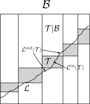
(a) Dividing ${\cal L}$ into strips

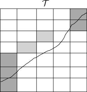
(b) The grid chain $\vec{{\cal D}}({\cal T})$

            

Figure 8: (a) The terminal chain $\vec{{\cal T}}$ is given by shaded boxes. The LIS ${\cal L}$ is depicted as a monotonically increasing freeform curve. (b) The grid chain $\vec{{\cal D}}({\cal T})$ is denoted by the shaded boxes. The set $\vec{{\cal E}}$ of boxes (not indicated explicitly) are the boxes intersecting the LIS that are not tainted.

For each terminal box ${\cal T}$:

• $\beta({\cal T})=|({\cal T}|{\cal B})\cap{\cal F}|$.

• ${\cal L}({\cal T})={\cal L}\cap({\cal T}|{\cal B})$.

• ${\cal L}^{in}({\cal T})={\cal L}\cap{\cal T}$.

• ${\cal L}^{out}({\cal T})={\cal L}\cap(({\cal T}|{\cal B})-{\cal T})$.

We give some notation regarding critical boxes.

• The concatenation of the $\vec{{\cal C}}({\cal T})$ for all ${\cal T}\in\vec{{\cal T}}$ is a box chain $\vec{{\cal C}}$ called the critical chain. Members of this chain are critical boxes.

• For index $x\in X({\cal B})$, $\vec{{\cal C}}[x]$ denotes the unique critical box ${\cal C}$ such that $x\in X({\cal C})$. Observe that for each $x\in F^{-1}({\cal B})$, the function ${\rm{\bf CriticalBox}}_{t}(x)$ returns ${\cal C}[x]$.

For each terminal box ${\cal T}$, let $\vec{{\cal D}}({\cal T})$ denote the grid chain of $\Gamma({\cal T})$ containing the maximum number of points from ${\cal L}$. Refer to [fig:critical]Fig. 8b. We will actually use the subsequence $\vec{{\cal E}}({\cal T})$, which consists of boxes ${\cal E}\in\vec{{\cal D}}({\cal T})$ such that ${\cal E}\cap{\cal L}\neq\emptyset$ and $({\cal E},t-1)$ is not tainted. The following quantities are used heavily in our proof.

• ${\tt out}(\vec{{\cal D}}({\cal T}))=\beta({\cal T})-\sum_{{\cal D}\in\vec{{\cal D}}({\cal T})}|{\cal D}\cap{\cal F}|$. (Number of ${\cal F}$-points in $({\cal T}|{\cal B})$ outside $\vec{{\cal D}}({\cal T})$.)

• ${\tt out}(\vec{{\cal E}}({\cal T}))=\beta({\cal T})-\sum_{{\cal E}\in\vec{{\cal E}}({\cal T})}|{\cal E}\cap{\cal F}|$. (Number of ${\cal F}$-points in $({\cal T}|{\cal B})$ outside $\vec{{\cal E}}({\cal T})$.)

• ${\tt loss}(\vec{{\cal E}}({\cal T}))=\sum_{{\cal E}\in\vec{{\cal E}}({\cal T})}{\tt loss}({\cal E})$. (Recall that ${\tt loss}({\cal E})=|{\cal E}\cap{\cal F}|-{\tt lis}({\cal E})]$, so ${\tt loss}(\vec{{\cal E}})$ is the number of ${\cal F}$-points from $\bigcup_{{\cal E}\in\vec{{\cal E}}({\cal T})}{\cal E}$ that are missed by the union of the LIS for ${\cal E}\in\vec{{\cal E}}({\cal T})$.)

• ${\tt aloss}_{t}(\vec{{\cal E}}({\cal T}))=\sum_{{\cal E}\in\vec{{\cal E}}({\cal T})}{\tt aloss}({\cal E})$. (Recall that ${\tt aloss}({\cal E})=[|{\cal E}\cap{\cal F}|-{\tt alis}_{t}({\cal E})]$ so ${\tt aloss}_{t}(\vec{{\cal E}}({\cal T}))$ is the estimate of ${\tt loss}(\vec{{\cal E}}({\cal T}))$ using ${\tt alis}_{t}$ in place of lis.)

We begin with a few simple propositions. The first, which follows immediately from the definition of ${\rm{\bf Classify}}$ specifies what happens in the base case $0pt({\cal B})=1$.

Proposition 14.

If ${\cal B}$ is a box of width 1, then ${\tt alis}_{t}({\cal B})={\tt lis}({\cal B})$ and $\nu_{t}({\cal B})=0$. For the unique $x\in X({\cal B})$, $x\in Good_{t}$ if and only if $F(x)\in{\cal B}$.

Henceforth, we assume that ${\cal B}$ has width at least 2. We remind that $Good_{t}({\cal B})$ denotes the set of indices ini $X({\cal B})$ classified as good by ${\rm{\bf Classify}}_{t}({\cal B})$. The quantity ${\tt alis}_{t}({\cal B})$ returned by the algorithm is an estimate of $|Good_{t}({\cal B})|$.

Proposition 15.

For any box ${\cal B}$ of width at least 2, and $t\geq 1$:

1. $Good_{t}({\cal B})$ is equal to the union over critical boxes ${\cal C}$ of $Good_{t-1}({\cal C})$.

2. $Good_{t}({\cal B})$ indexes an increasing sequence in ${\cal B}$ and thus $|Good_{t}({\cal B})|\leq{\tt lis}({\cal B})$.

Proof 8.3.

The first part follows from the main case of ${\rm{\bf Classify}}_{t}$. For the second part, if $x,y\in Good_{t}({\cal B})$ then either $F(x)$ and $F(y)$ belong to different boxes of $\vec{{\cal C}}$ or $F(x),F(y)$ lie in the same critical box ${\cal C}$. In the former case, they are comparable since the boxes lie in a box chain. In the latter case, they are both classified good by ${\rm{\bf Classify}}_{t-1}(\cdot,{\cal C})$ and must be comparable by induction on $t$.

8.2 Components of secondary error

In this section we identify five components of secondary error, denoted $\zeta_{1},\ldots,\zeta_{5}$. We gather the definitions together here for easy reference, but the motivation for each term comes from the analysis presented in Section 8.4.

$$\zeta_{1}={\tt alis}_{t}({\cal B})-|Good_{t}({\cal B})|.$$

Recall that the subroutine ${\rm{\bf TerminalBox}}_{t}$ together with the secondary random bits determine the terminal box chain $\vec{{\cal T}}$. The remaining four secondary error terms are associated to each individual terminal box ${\cal T}$ in $\vec{{\cal T}}$; the secondary error will be obtained by summing these over all ${\cal T}$. We define:

$$\zeta_{2}({\cal T}) = \sum_{{\cal C}\in\vec{{\cal C}}({\cal T})}{\tt alis}_{t-1}({\cal C})-\sum_{{\cal C}\in\vec{{\cal C}}({\cal T})}|Good_{t-1}({\cal C})|.$$

$$\zeta_{3}({\cal T}) = |{\cal L}^{in}({\cal T})|-\sum_{{\cal E}\in\vec{{\cal E}}({\cal T})}|{\cal E}\cap{\cal L}|.$$

$$\zeta_{4}({\cal T}) = |{\cal L}^{out}({\cal T})|-\mu_{t}\cdot{\tt out}(\vec{{\cal E}}({\cal T})).$$

$$\zeta_{5}({\cal T}) = \mu_{t}\cdot{\tt aloss}_{t-1}(\vec{{\cal E}}({\cal T}))-(1-\mu_{t})\cdot{\tt out}(\vec{{\cal E}}({\cal T})).$$

8.3 Transforming our goal

Our goal is to upper bound $|\nu_{t}({\cal B})|=|{\tt lis}({\cal B})-{\tt alis}_{t}({\cal B})|$. We start from the definition of $\nu_{t}({\cal B})$, substitute $|Good_{t}({\cal B})|+\zeta_{1}$ for ${\tt alis}_{t}({\cal B})$ and apply the inequality (from [prop:good]Prop. 15) ${\tt lis}({\cal B})\geq Good_{t}({\cal B})$:

$$|\nu_{t}({\cal B})| = |{\tt lis}({\cal B})-{\tt alis}_{t}({\cal B})|$$

$$= |{\tt lis}({\cal B})-|Good_{t}({\cal B})|-\zeta_{1}|$$

$$\leq {\tt lis}({\cal B})-|Good_{t}({\cal B})|+|\zeta_{1}|$$

Define:

$$\Delta_{t}={\tt lis}({\cal B})-|Good_{t}({\cal B})|-\tau_{t}{\tt loss}({\cal B}),$$

Our goal (1) will follow from:

$$\Delta_{t}\leq\delta_{t}0pt({\cal B})-|\zeta_{1}|.$$

Noting that ${\tt lis}({\cal B})=|{\cal L}|$ and ${\tt loss}({\cal B})=|{\cal B}\cap{\cal F}|-|{\cal L}|$. we have:

$$\Delta_{t}=(1+\tau_{t})|{\cal L}|-|Good_{t}({\cal B})|-\tau_{t}|{\cal B}\cap{\cal F}|$$

Each term on the right counts a subset of ${\cal B}\cap{\cal F}$. Partitioning the box ${\cal B}$ into the strips $({\cal T}|{\cal B})$ for each terminal box ${\cal T}$, we define $\Delta_{t}({\cal T})$ as follows to be the contribution of the points in ${\cal T}|{\cal B}$ to the right hand side (using the notation in Section 8.1 and noting that $Good_{t}({\cal B})\cap({\cal T}|{\cal B})\subseteq{\cal T}$):

$$\Delta_{t}({\cal T}) =(1+\tau_{t})|{\cal L}({\cal T})|-|Good_{t}({\cal B})\cap{\cal T}|-\tau_{t}\beta({\cal T})$$ (2)

Our goal now is to show:

$$\sum_{{\cal T}\in\vec{{\cal T}}}\Delta_{t}(T) \leq \delta_{t}0pt({\cal B})-|\zeta_{1}|.$$ (3)

This is broken down into two steps. We use the notation $x^{+}=\max(x,0)$.

Claim 16.

(Primary error) Let $t\geq 1$ and let ${\cal B}$ be a box such that $({\cal B},t)$ is untainted. Let $\vec{{\cal T}}$ be the terminal chain associated with a call of ${\rm{\bf ApproxLIS}}_{t}({\cal B})$. We have:

$$\sum_{{\cal T}\in\vec{{\cal T}}}\Delta_{t}({\cal T}) \leq (\delta_{t}-\delta_{1})0pt({\cal B})+\sum_{{\cal T}\in\vec{{\cal T}}}(\zeta_{2}({\cal T})+5\zeta_{3}({\cal T})^{+}+5\zeta_{4}({\cal T})^{+}+2\zeta_{5}({\cal T})^{+}).$$ (4)

Claim 17.

(Secondary error) With the same hypotheses as in Claim 16 together with Assumption 1, we have:

$$|\zeta_{1}|+\sum_{{\cal T}\in\vec{{\cal T}}}(\zeta_{2}({\cal T})+5\zeta_{3}({\cal T})^{+}+5\zeta_{4}({\cal T})^{+}+2\zeta_{5}({\cal T})^{+}) \leq \delta_{1}0pt({\cal B}).$$ (5)

Summing these bounds yields [eq:goal12.1](3), which proves [thm:basic correctness]Thm. 8.1.

8.4 Bounding the primary error

Here we prove Claim 16. The proof is by induction on $t$. The base case is $t=1$. We prove the base case and the induction step together, indicating where they differ.

The following claim bounds $\Delta_{t}({\cal T})$ in a more convenient form.

Claim 18.

For each terminal box ${\cal T}$,

$$\Delta_{t}({\cal T}) \leq (1+\tau_{t})|{\cal L}^{out}({\cal T})|-\tau_{t}\cdot{\tt out}(\vec{{\cal E}}({\cal T}))-(1+\tau_{t})\cdot{\tt loss}(\vec{{\cal E}}({\cal T}))+{\tt aloss}_{t-1}(\vec{{\cal E}}({\cal T}))$$

$$+\zeta_{2}({\cal T})+(1+\tau_{t})\zeta_{3}({\cal T}).$$

Proof 8.4.

By Proposition 15, $|Good_{t}({\cal B})\cap{\cal T}|=\sum_{{\cal C}\in\vec{{\cal C}}({\cal T})}|Good_{t-1}({\cal C})|$. Thus, (2) can be rewritten as:

$$\Delta_{t}({\cal T}) = (1+\tau_{t})|{\cal L}({\cal T})|-\sum_{{\cal C}\in\vec{{\cal C}}({\cal T})}|Good_{t-1}({\cal C})|-\tau_{t}\beta({\cal T})$$

We replace $|Good_{t-1}({\cal C})|$ by ${\tt alis}_{t-1}({\cal C})$, using $\zeta_{2}({\cal T})$.

$$\Delta_{t}({\cal T}) = (1+\tau_{t})|{\cal L}({\cal T})|-\sum_{{\cal C}\in\vec{{\cal C}}({\cal T})}{\tt alis}_{t-1}({\cal C})-\tau_{t}\beta({\cal T})+\zeta_{2}({\cal T})$$

By construction, $\vec{{\cal C}}({\cal T})$ is a grid-chain with respect to the grid $\Gamma({\cal T})$ that maximizes the sum $\sum_{{\cal C}\in\vec{{\cal C}}({\cal T})}{\tt alis}_{t-1}({\cal C})$. This sum is at least $\sum_{{\cal E}\in\vec{{\cal E}}({\cal T})}{\tt alis}_{t-1}({\cal E})$, since $\vec{{\cal E}}$ is a subsequence of a grid-chain.

$$\Delta_{t}({\cal T}) \leq (1+\tau_{t})|{\cal L}({\cal T})|-\sum_{{\cal E}\in\vec{{\cal E}}({\cal T})}{\tt alis}_{t-1}({\cal E})-\tau_{t}\beta({\cal T})+\zeta_{2}({\cal T})$$

Now, $|{\cal L}({\cal T})|=|{\cal L}^{in}({\cal T})|+|{\cal L}^{out}({\cal T})|$. Using the definition of $\zeta_{3}({\cal T})$, $|{\cal L}^{in}|=\zeta_{3}({\cal T})+\sum_{{\cal E}\in\vec{{\cal E}}({\cal T})}|{\cal E}\cap{\cal L}|$; the grid approximation lemma ([lem:grid-approx]Lem. 5.12) will be used to show that $\zeta_{3}({\cal T})$ is small. Furthermore, for each ${\cal E}\in\vec{{\cal E}}({\cal T})$, $|{\cal E}\cap{\cal L}|\leq{\tt lis}({\cal E})$. Combining,

$$\Delta_{t}({\cal T}) \leq (1+\tau_{t})|{\cal L}^{out}({\cal T})|+(1+\tau_{t})\sum_{{\cal E}\in\vec{{\cal E}}({\cal T})}{\tt lis}({\cal E})-\sum_{{\cal E}\in\vec{{\cal E}}({\cal T})}{\tt alis}_{t-1}({\cal E})-\tau_{t}\beta({\cal T})$$

$$+\zeta_{2}({\cal T})+(1+\tau_{t})\zeta_{3}({\cal T})$$

Substituting ${\tt lis}({\cal E})=|{\cal E}\cap{\cal F}|-{\tt loss}({\cal E})$, and ${\tt alis}_{t}({\cal E})=|{\cal E}\cap{\cal F}|-{\tt aloss}({\cal E})$ and performing some simple algebraic manipulations completes the proof:

$$\Delta_{t}({\cal T}) \leq (1+\tau_{t})|{\cal L}^{out}({\cal T})|+(1+\tau_{t})\Big{[}\sum_{{\cal E}\in\vec{{\cal E}}({\cal T})}|{\cal E}\cap{\cal F}|-{\tt loss}(\vec{{\cal E}}({\cal T}))\Big{]}-\Big{[}\sum_{{\cal E}\in\vec{{\cal E}}({\cal T})}|{\cal E}\cap{\cal F}|-{\tt aloss}_{t-1}(\vec{{\cal E}}({\cal T}))\Big{]}$$

$$-\tau_{t}\beta({\cal T})+\zeta_{2}({\cal T})+(1+\tau_{t})\zeta_{3}({\cal T})$$

$$= (1+\tau_{t})|{\cal L}^{out}({\cal T})|-\tau_{t}\Big{[}\beta({\cal T})-\sum_{{\cal E}\in\vec{{\cal E}}({\cal T})}|{\cal E}\cap{\cal F}|\Big{]}-(1+\tau_{t})\cdot{\tt loss}(\vec{{\cal E}}({\cal T}))+{\tt aloss}_{t-1}(\vec{{\cal E}}({\cal T}))$$

$$+\zeta_{2}({\cal T})+(1+\tau_{t})\zeta_{3}({\cal T})$$

$$= (1+\tau_{t})|{\cal L}^{out}({\cal T})|-\tau_{t}\cdot{\tt out}(\vec{{\cal E}}({\cal T}))-(1+\tau_{t})\cdot{\tt loss}(\vec{{\cal E}}({\cal T}))+{\tt aloss}_{t-1}(\vec{{\cal E}}({\cal T}))$$

$$+\zeta_{2}({\cal T})+(1+\tau_{t})\zeta_{3}({\cal T}).$$

Claim 19.

${\tt loss}(\vec{{\cal E}}({\cal T}))\geq K_{t}[{\tt aloss}_{t-1}(\vec{{\cal E}}({\cal T}))-\delta_{t-1}0pt({\cal T})]$, where $K_{1}=0$ and $K_{t}=1/(1+\tau_{t-1})$ for $t\geq 2$.

Proof 8.5.

For $t=1$, simply note that the loss is always non-negative.

Suppose $t\geq 2$. By construction of $\vec{{\cal E}}$, for each ${\cal E}\in\vec{{\cal E}}$, $({\cal E},t-1)$ is not tainted. Using the induction hypothesis, we can relate ${\tt loss}({\cal E})$ to ${\tt aloss}_{t-1}({\cal E})$. The proof is completed by summing the following bound over all ${\cal E}\in\vec{{\cal E}}({\cal T})$.

$${\tt aloss}_{t-1}({\cal E})\leq(1+\tau_{t-1}){\tt loss}({\cal E})+\delta_{t-1}0pt({\cal E})$$

$$\Longleftrightarrow{\tt loss}({\cal E})\geq\frac{{\tt aloss}_{t-1}({\cal E})}{1+\tau_{t-1}}-\frac{\delta_{t-1}0pt({\cal E})}{1+\tau_{t-1}}$$

Combining this claim with [clm:delta]Claim 18 gives:

$$\Delta_{t}({\cal T}) \leq (1+\tau_{t})|{\cal L}^{out}({\cal T})|-\tau_{t}\cdot{\tt out}(\vec{{\cal E}}({\cal T}))+[1-K_{t}(1+\tau_{t})]\cdot{\tt aloss}_{t-1}(\vec{{\cal E}}({\cal T}))$$

$$+\zeta_{2}({\cal T})+(1+\tau_{t})\zeta_{3}({\cal T})+K_{t}\delta_{t-1}0pt({\cal T}).$$

We use $\zeta_{4}({\cal T})$ and $\zeta_{5}({\cal T})$ to eliminate $|{\cal L}^{out}|$ and ${\tt aloss}_{t-1}(\vec{{\cal E}}({\cal T}))$.

$$\Delta_{t}({\cal T}) \leq (1+\tau_{t})[\mu_{t}\cdot{\tt out}(\vec{{\cal E}}({\cal T}))+\zeta_{4}({\cal T})]-\tau_{t}\cdot{\tt out}(\vec{{\cal E}}({\cal T}))+$$ (6)

$$[1-K_{t}(1+\tau_{t})]\mu^{-1}_{t}[(1-\mu_{t})\cdot{\tt out}(\vec{{\cal E}}({\cal T}))+\zeta_{5}({\cal T})]+\zeta_{2}({\cal T})+(1+\tau_{t})\zeta_{3}({\cal T})+K_{t}\delta_{t-1}0pt({\cal T})$$

$$= [(1+\tau_{t})\mu_{t}-\tau_{t}+(1-K_{t}(1+\tau_{t}))(\mu^{-1}_{t}-1)]{\tt out}(\vec{{\cal E}}({\cal T}))$$

$$+\zeta_{2}({\cal T})+(1+\tau_{t})\zeta_{3}({\cal T})+(1+\tau_{t})\zeta_{4}({\cal T})+[1-K_{t}(1+\tau_{t})]\mu^{-1}_{t}\zeta_{5}({\cal T})+K_{t}\delta_{t-1}0pt({\cal T})$$

Our focus is on the coefficient of ${\tt out}(\vec{{\cal E}}({\cal T}))$ and the parameters will be chosen to ensure this is negative.

$$(1+\tau_{t})\mu_{t}-\tau_{t}+[1-K_{t}(1+\tau_{t})](\mu^{-1}_{t}-1)$$

$$= (1+\tau_{t})\mu_{t}-(1+\tau_{t})+K_{t}(1+\tau_{t})+[1-K_{t}(1+\tau_{t})]\mu^{-1}_{t}$$

$$= \mu^{-1}_{t}[(1+\tau_{t})\mu^{2}_{t}-(1+\tau_{t})(1-K_{t})\mu_{t}-K_{t}(1+\tau_{t})+1]$$

$$= \mu^{-1}_{t}\{(1+\tau_{t})[\mu^{2}_{t}-(1-K_{t})\mu_{t}-K_{t}]+1\}$$

Setting $\mu_{t}=(1-K_{t})/2$ (which is positive since $K_{t}<1$) minimizes the inner quadratic. The condition that this expression is non-positive is equivalent to the following.

$$(1+\tau_{t})[(1-K_{t})^{2}/4-(1-K_{t})^{2}/2-K_{t}]\leq-1\Longleftrightarrow(1+\tau_{t})\geq\frac{4}{(1+K_{t})^{2}}$$

For $t=1$, we have $K_{t}=0$ and the requirement is $\tau_{t}\geq 3$. For $t\geq 2$, $K_{t}=1/(1+\tau_{t-1})$ and the requirement becomes:

$$\tau_{t}\geq\frac{4\tau_{t-1}+3\tau^{2}_{t-1}}{(2+\tau_{t-1})^{2}}$$

Guessing a solution of the form $\tau_{t}=C/t$, one verifies that $\tau_{t}=4/t$ works. The righthand side becomes

$$\frac{\frac{16}{t-1}+\frac{48}{(t-1)^{2}}}{(2+\frac{4}{t-1})^{2}}=\frac{16(t-1)+48}{(2(t-1)+4)^{2}}=\frac{4t+8}{(t+1)^{2}}\leq\frac{4t+8+\frac{4}{t}}{(t+1)^{2}}=\frac{4}{t}.$$

Thus the coefficient of ${\tt out}(\vec{{\cal E}}(T))$ in [eq:errors](6) is nonpositive. To further simplify the bound note that $K_{t}=(t-1)/(t+3)\leq 1$ and $(1-K_{t}(1+\tau_{t}))/\mu_{t}=2(1-K_{t}(1+\tau_{t}))/(1-K_{t})\leq 2$. Thus from [eq:errors](6) we deduce:

$$\Delta_{t}({\cal T}) \leq \zeta_{2}({\cal T})+(1+\tau_{t})\zeta_{3}({\cal T})+(1+\tau_{t})\zeta_{4}({\cal T})+\zeta_{5}({\cal T})(1-K_{t}(1+\tau_{t}))/\mu_{t}+K_{t}\delta_{t-1}0pt({\cal T})$$

$$\leq \zeta_{2}({\cal T})+5\zeta_{3}({\cal T})+5\zeta_{4}({\cal T})+2\zeta_{5}({\cal T})+(\delta_{t}-\delta_{1})0pt({\cal T}).$$

Summing over ${\cal T}$ completes the proof of the claim.

Remark. The reader should note that in the proof of [clm:primary]Claim 16, the only thing used about the algorithm ${\rm{\bf TerminalBox}}$ is [lem:terminal]Lem. 7.4. The exact details of how the terminal chain was chosen are not used. Similarly, the particular choice of $\delta_{1}$ was not used; we only use the fact that $\delta_{t}=t\delta_{1}$. The assumptions on the random seed are just Assumption 1 and that fact that $({\cal B},t)$ is not tainted. The specifics of the definition of tainted do no enter this proof. All the calculations were basically algebraic manipulations (most details about the algorithm have been pushed into the secondary error terms). We mention this because our improved algorithm will be obtained by modifying ${\rm{\bf TerminalBox}}$ and changing $\delta_{1}$ (but not $\tau_{t}$ or $\mu_{t}$). In analyzing the quality of approximation in the second algorithm, we can reuse the analysis of this section.

8.5 Bounding the secondary error terms

In this section we prove [clm:secondary]Claim 17. We examine each of the error terms separately and show that each one contributes at most $\frac{1}{5\log(n)}=\frac{\delta_{1}}{5}$ to the secondary error, and so the total secondary error is at most $\delta_{1}$.

Claim 20.

If $({\cal B},t)$ is not tainted, $|\zeta_{1}|\leq\eta 0pt({\cal B})$ and $\sum_{\cal T}\zeta_{2}({\cal T})\leq 2\eta 0pt({\cal B})$.

Proof 8.6.

The first inequality follows immediately from the definition of (non)tainted boxes: $|\zeta_{1}|=|{\tt alis}_{t}({\cal B})-|Good_{t}({\cal B})||\leq\eta 0pt({\cal B})$.

For the second inequality, recall that $\vec{{\cal C}}$ is the critical chain for ${\cal B}$ and $\vec{{\cal C}}({\cal T})$ is the portion of the critical chain in terminal box ${\cal T}$. Let $\vec{{\cal C}}^{*}\subset\vec{{\cal C}}$ be the set of critical boxes ${\cal C}\in\vec{{\cal C}}$ such that $({\cal C},t-1)$ is tainted. Since $({\cal B},t)$ is not tainted, $\sum_{{\cal C}\in\vec{{\cal C}}^{*}}0pt({\cal C})\leq\eta 0pt({\cal B})$. We therefore have:

$$\sum_{\cal T}\zeta_{2}({\cal T}) = \sum_{{\cal C}\in\vec{{\cal C}}}{\tt alis}({\cal C})-|Good_{t-1}({\cal C})|$$

$$\leq \sum_{{\cal C}\in\vec{{\cal C}}}|{\tt alis}({\cal C})-|Good_{t-1}({\cal C})||$$

$$\leq \sum_{{\cal C}\in\vec{{\cal C}}^{*}}0pt({\cal C})+\sum_{{\cal C}\in\vec{{\cal C}}-\vec{{\cal C}}^{*}}\eta 0pt({\cal C})$$

$$\leq \eta 0pt({\cal B})+\eta 0pt({\cal B})\ =2\eta 0pt({\cal B}).$$

Since $\eta=1/10\log(n)$, both $|\zeta_{1}|$ and $\sum_{{\cal T}\in\vec{{\cal T}}}\zeta_{2}({\cal T})$ are bounded above by $0pt({\cal B})/(5\log n)$.

We move on to the error term $\zeta_{3}({\cal T})=|{\cal L}^{in}({\cal T})|-\sum_{{\cal E}\in\vec{{\cal E}}({\cal T})}|{\cal E}\cap{\cal L}|.$

Claim 21.

$$\sum_{{\cal T}\in\vec{{\cal T}}}\zeta_{3}({\cal T}) \leq (\alpha+\eta)0pt({\cal B}).$$

Proof 8.7.

Focus on a single terminal box ${\cal T}$. By the grid approximation lemma ([lem:grid-approx]Lem. 5.12), we can choose the chain $\vec{{\cal D}}({\cal T})$ so that it misses at most $\alpha 0pt({\cal T})$ points of ${\cal L}^{in}({\cal T})$. (Note that $\vec{{\cal E}}$ is the subsequence consisting of non-tainted boxes.) Let the total width of the tainted boxes in $\vec{{\cal D}}({\cal T})$ be denoted as $b({\cal T})$. Hence, $\zeta_{3}({\cal T})\leq\alpha 0pt({\cal T})+b({\cal T})$. Summing over all ${\cal T}$, $\sum_{{\cal T}\in\vec{{\cal T}}}\zeta_{3}({\cal T})\leq\alpha 0pt({\cal B})+\sum_{{\cal T}\in\vec{{\cal T}}}b({\cal T})$. Since $({\cal B},t)$ is not tainted, the latter sum is at most $\eta 0pt({\cal B})$.

Substituting $\alpha=1/(C_{1}\log n)^{3}$ and $\eta=1/(10\log n)$, gives $\sum_{{\cal T}\in\vec{{\cal T}}}\zeta_{3}({\cal T})\leq 0pt({\cal B})/(5\log n)$.

Next we consider the error term $\zeta_{4}({\cal T})=|{\cal L}_{out}({\cal T})|-\mu_{t}\cdot{\tt out}(\vec{{\cal E}}({\cal T}))$.

Claim 22.

$$\sum_{{\cal T}\in\vec{{\cal T}}}\zeta_{4}({\cal T}) \leq \Big{(}2\alpha+\frac{4\gamma\log n}{\rho}\Big{)}0pt({\cal B})\leq 0pt({\cal B})/(5\log n).$$

The main part of the claim is [lem:et4]Lem. 8.8, which is formulated more generally to allow for its reuse later. Recall that in [sec:terminal]§7.2, we constructed a tree associated with calls to ${\rm{\bf TerminalBox}}_{t}(\cdot,{\cal B})$ whose leaves were the terminal boxes and whose intermediate nodes were boxes that occur along some execution of ${\rm{\bf TerminalBox}}_{t}(\cdot,{\cal B})$. Each intermediate node was also associated to a unique splitter selected to split the associated box. These splitters make up the interior increasing point sequence ${\cal P}^{\circ}(\vec{{\cal T}})$ associated with the terminal chain $\vec{{\cal T}}$. For each $P\in{\cal P}^{\circ}(\vec{{\cal T}})$ we defined ${\cal H}(P)$ to be the box in the splitter tree that was split by $P$, and noted that by Assumption 1, $P$ is $(\mu_{t},2\gamma 0pt({\cal H}(P)))$-safe for ${\cal H}(P)$.

In the improved algorithm to be presented in [sec:improved]§9, the parameter $\gamma$ will not be fixed, and the splitter selected for different boxes may be selected based on a different $\gamma$. To anticipate this we introduce the notation $\gamma(P)$ to be the value of $\gamma$ that was used when $P$ was selected as splitter for ${\cal H}(P)$ and so Assumption 1 gives that $P$ is a $(\mu_{t},2\gamma(P)0pt({\cal H}(P)))$-splitter for ${\cal H}(P)$. Nothing in the previous analysis relied on $\gamma$ being fixed (indeed, this is the first time in the proof of [thm:basic correctness]Thm. 8.1 that $\gamma$ has been used.)

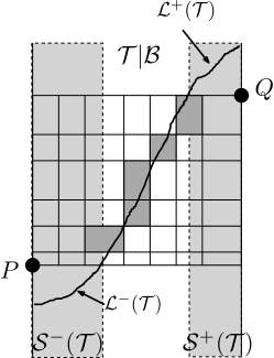
Figure 9: The LIS ${\cal L}$ is depicted as a monotonically increasing freeform curve. The boxes in $\vec{{\cal E}}$ are colored dark gray, and the strips ${\cal S}^{-}({\cal T})$, ${\cal S}^{+}({\cal T})$ are in light gray.

Lemma 8.8.

$$\sum_{{\cal T}\in\vec{{\cal T}}}\zeta_{4}({\cal T}) \leq 2\alpha 0pt({\cal B})+4\sum_{P\in{\cal P}^{\circ}(\vec{{\cal T}})}\gamma(P)0pt({\cal H}(P)).$$

Proof 8.9.

Looking at the definition of $\zeta_{4}({\cal T})$, our first goal is to obtain a lower bound on ${\tt out}(\vec{{\cal E}}({\cal T}))=\beta({\cal T})-\sum_{{\cal E}\in\vec{{\cal E}}({\cal T})}|{\cal E}\cap{\cal F}|$, the number of ${\cal F}$-points in the strip ${\cal T}|{\cal B}$ that lie outside of $\vec{{\cal E}}$.

Note that ${\cal L}^{out}({\cal T})$ can be split into the set ${\cal L}^{-}({\cal T})$ of points that lie below ${\cal T}$ and ${\cal L}^{+}({\cal T})$ of points that lie above ${\cal T}$. Refer to [fig:et4]Fig. 9. Let ${\cal S}^{-}({\cal T})$ be the smallest strip starting from the left edge of ${\cal T}|{\cal B}$ that contains all of ${\cal L}^{-}({\cal T})$ (so ${\cal S}^{-}({\cal T})$ is either empty, or has its rightmost edge defined by the largest $x$ for which $F(x)\in{\cal L}$ and lies below ${\cal T}$). Similarly, let ${\cal S}^{+}({\cal T})$ be the smallest strip that ends at the right edge of ${\cal T}|{\cal B}$ and contains all of ${\cal L}^{+}({\cal T})$. Since ${\cal L}$ is increasing, ${\cal S}^{-}({\cal T})$ and ${\cal S}^{+}({\cal T})$ are disjoint.

The overlap of ${\cal S}^{-}({\cal T})\cup{\cal S}^{+}({\cal T})$ with $\vec{{\cal E}}({\cal T})^{\cup}$ is small. We claim that only the leftmost box ${\cal E}_{L}$ of $\vec{{\cal E}}$ can overlap ${\cal S}^{-}({\cal T})$ (and a similar argument shows that only the rightmost box ${\cal E}_{R}$ can overlap ${\cal S}^{+}({\cal T})$). The right edge of ${\cal S}^{-}({\cal T})$ occurs at the rightmost point of ${\cal L}^{-}$. The right edge of ${\cal E}_{L}$ must be to the right of that because ${\cal E}_{L}$ contains at least one point in ${\cal L}^{in}$. Hence,

$${\tt out}(\vec{{\cal E}}({\cal T})) \geq |({\cal S}^{-}({\cal T})\cup{\cal S}^{+}({\cal T}))\cap{\cal F}|-|({\cal E}_{L}\cup{\cal E}_{R})\cap{\cal F}|$$

$$\geq |({\cal S}^{-}({\cal T})\cup{\cal S}^{+}({\cal T}))\cap{\cal F}|-2\alpha 0pt({\cal T}),$$

where the second inequality uses the fact that each of the grid strips of ${\cal T}|{\cal B}$ have width at most $\alpha 0pt({\cal T})$. We now have:

$$\zeta_{4}({\cal T}) = |{\cal L}^{out}({\cal T})|-\mu_{t}\cdot{\tt out}(\vec{{\cal E}}({\cal T}))$$

$$\leq |{\cal L}^{-}({\cal T})|+|{\cal L}^{+}({\cal T})|-\mu_{t}(|({\cal S}^{-}({\cal T})\cup{\cal S}^{+}({\cal T}))\cap{\cal F}|-2\alpha 0pt({\cal T}))$$

$$\leq (|{\cal L}^{-}({\cal T})|-\mu_{t}|{\cal S}^{-}({\cal T})\cap{\cal F}|)+(|{\cal L}^{+}({\cal T})|-\mu_{t}|{\cal S}^{+}({\cal T})\cap{\cal F}|)+2\mu_{t}\alpha 0pt({\cal T}).$$

We now bound the first two terms in the final expression. Let $P$ be the bottom left point of ${\cal T}$ and $Q$ be the top right point of ${\cal T}$. All of the points in ${\cal L}^{-}({\cal T})$ are in violation with $P$. (Refer to [fig:et4]Fig. 9.) Since $P$ is a $(\mu_{t},2\gamma(P)0pt({\cal H}(P)))$-splitter for ${\cal H}(P)$, there are at most $\mu|{\cal S}^{-}({\cal T})\cap{\cal F}|+2\gamma(P)0pt({\cal H}(P))$ points of ${\cal F}$ that are in violation with $P$ and so $|{\cal L}^{-}({\cal T})|-\mu|{\cal S}^{-}({\cal T})\cap{\cal F}|\leq 2\gamma(P)0pt({\cal H}(P))$. Similarly $|{\cal L}^{+}({\cal T})|-\mu|{\cal S}^{+}({\cal T})\cap{\cal F}|\leq 2\gamma(Q)0pt({\cal H}(Q))$. Thus:

$$\zeta_{4}({\cal T}) \leq 2\gamma(P)0pt({\cal H}(P))+2\gamma(Q)0pt({\cal H}(Q))+2\mu_{t}\alpha 0pt({\cal T}).$$

Finally, we sum the inequality in the lemma over all terminal boxes ${\cal T}$. Observing that $\mu_{t}\leq 1$ and that each point $P$ of the point sequence ${\cal P}^{\circ}(\vec{{\cal T}})$ gets included twice (once as a bottom left point and once as an upper right point), we get:

$$\sum_{{\cal T}\in\vec{{\cal T}}^{w}}\zeta_{4}({\cal T}) \leq 2\alpha 0pt({\cal B})+4\sum_{P\in{\cal P}^{\circ}(\vec{{\cal T}})}\gamma(P)0pt({\cal H}(P)).$$

Proof 8.10 (of [clm:et4]Claim 22).

We use the previous lemma with $\gamma(P)=\gamma$ for all $P$. For a given level of the splitter tree the sum of $0pt({\cal H})$ is equal to $0pt({\cal B})$ so the total sum is bounded by $0pt({\cal B})d$ where $d$ is the depth of the splitter tree. Since each splitter is $\rho$-balanced, the width of a box at depth $d$ in the splitter tree is at most $n(1-\rho)^{d}\leq ne^{-\rho d}$. This must be at least 1, so $d\leq(\log n)/\rho$. Thus we have:

$$\sum_{{\cal T}\in\vec{{\cal T}}}\zeta_{4}({\cal T}) \leq \Big{(}2\alpha+\frac{4\gamma(\log n)}{\rho}\Big{)}0pt({\cal B}).$$ (7)

Applying $\rho=C_{1}/\log n$ and $\alpha=\gamma=(1/C_{1}\log n)^{3}$, we get the final inequality.

Finally, we consider $\zeta_{5}({\cal T})=\mu_{t}\cdot{\tt aloss}_{t-1}(\vec{{\cal E}}({\cal T}))-(1-\mu_{t})\cdot{\tt out}(\vec{{\cal E}}({\cal T}))$. Let us review the basic terms. We have a terminal box ${\cal T}$ inside ${\cal B}$ andgrid $\Gamma({\cal T})$. $\vec{{\cal D}}({\cal T})$ is the grid-chain with the largest number of points in ${\cal L}$. Tainted boxes and those containing no point of ${\cal L}$ are removed from $\vec{{\cal D}}({\cal T})$ to get the chain $\vec{{\cal E}}({\cal T})$.

Proposition 8.11.

$\zeta_{5}({\cal T})\leq\mu_{t}\cdot{\tt aloss}_{t-1}(\vec{{\cal D}}({\cal T}))-(1-\mu_{t})\cdot{\tt out}(\vec{{\cal D}}({\cal T}))$.

Proof 8.12.

Since $\vec{{\cal E}}({\cal T})$ is a subsequence of $\vec{{\cal D}}({\cal T})$, ${\tt aloss}_{t-1}(\vec{{\cal E}}({\cal T}))\leq{\tt aloss}_{t-1}(\vec{{\cal D}}({\cal T}))$ and ${\tt out}(\vec{{\cal E}}({\cal T}))\geq{\tt out}(\vec{{\cal D}}({\cal T}))$.

Claim 23.

For every terminal box ${\cal T}$, if ${\cal T}$ is narrow then $\zeta_{5}({\cal T})\leq 0$ and if $\zeta_{5}({\cal T})$ is wide then $\zeta_{5}({\cal T})\leq 4\rho 0pt({\cal T})\leq\frac{1}{5\log(n)}0pt({\cal T})$.

Proof 8.13.

For convenience, we abbreviate $\vec{{\cal D}}({\cal T})$ by $\vec{{\cal D}}$. We apply [lem:dichotomy]Lem. 5.7 to the box ${\cal T}|{\cal B}$ with the strip decomposition given by the grid $\Gamma({\cal T})$. We get $(1-\mu_{t})\cdot{\tt out}(\vec{{\cal D}})\geq\mu_{t}\cdot|U|$, where $U$ is the set of $\vec{{\cal D}}$-points that are $\mu_{t}$-unsafe in $\Gamma({\cal T})$. Hence, $\zeta_{5}({\cal T})\leq\mu_{t}({\tt aloss}_{t-1}(\vec{{\cal D}})-|U|)$.

Suppose ${\cal T}$ is narrow (that is, $0pt({\cal T})\leq 1/\rho$). By the definition of ${\rm{\bf BuildGrid}}$, the grid $\Gamma({\cal T})$ has $X(\Gamma({\cal T}))=X({\cal T})$, and so each box ${\cal D}\in\vec{{\cal D}}$ has width 1. For any such box ${\tt alis}_{t-1}({\cal D})=|{\cal D}\cap{\cal F}|$, so ${\tt aloss}_{t-1}({\cal D})=0$. Hence, $\zeta_{5}({\cal T})\leq 0$.

Suppose ${\cal T}$ is wide (that is, $0pt({\cal T})>1/\rho$). We can crudely bound ${\tt aloss}_{t-1}(\vec{{\cal D}})\leq|\vec{{\cal D}}^{\cup}\cap{\cal F}|$, so $\zeta_{5}\leq\mu_{t}|S|$, where $S$ is the set of ${\cal D}$-points that are $\mu_{t}$-safe in $\Gamma({\cal T})$.

Every box in $\vec{{\cal D}}$ has width at most $\alpha 0pt({\cal T})\leq\gamma 0pt({\cal T})$ (since $\vec{{\cal D}}$ is a $\Gamma({\cal T})$-chain). So any $\mu_{t}$-safe point in $\Gamma({\cal T})$ is $(\mu_{t},\gamma 0pt({\cal T}))$-safe. ${\cal T}$ is a wide terminal box and ${\rm{\bf FindSplitter}}_{t}({\cal T},{\cal B},\mu_{t},\gamma 0pt({\cal T}),\rho)$ failed to find a splitter. By Assumption 1 (reliability of ${\rm{\bf FindSplitter}})$ and [cor:fails]Cor. 5.4, the total number of nondegenerate $(\mu_{t},\gamma 0pt({\cal T}))$-safe indices for ${\cal T}|{\cal B}$ is at most $3\rho 0pt({\cal T})$. Therefore, $|S|\leq 3\rho 0pt({\cal T})+1\leq 4\rho 0pt({\cal T})$ (where the last inequality follows from the fact that ${\cal T}$ is wide), completing the proof.

We have thus shown that each of the five error terms is bounded by $0pt({\cal B})/5\log(n)$ and so the total secondary error is $0pt({\cal B})/\log(n)=\delta_{1}0pt({\cal B})$. This completes the proof of [clm:secondary]Claim 17 the approximation error bound for the first algorithm.

9 The improved algorithm

The previous algorithm had running time $(\log n)^{O(1/\overline{\tau})}$ where $\tau$ is the primary approximation parameter. In this section we show how to modify the algorithm so that the running time is $(1/\overline{\delta}\overline{\tau})^{O(1/\overline{\tau})}(\log n)^{c}$ for some absolute constant $c$, where $\overline{\delta}$ is the secondary error parameter, thereby proving [thm:alg2]Thm. 4.2. The improved running time is obtained by making some subtle (and somewhat mysterious) changes to the basic algorithm. Formally the changes are minor, and we will start by completely describing the revisions made to the basic algorithm without motivating the reasons for the changes. Then we provide an informal discussion of how we arrived at these changes. (The reader may wish to read this discussion before reading the formal description.) Finally we prove the properties of the improved algorithm.

9.1 Formal description of the algorithm

The basic algorithm consists of 6 main procedures,${\rm{\bf BasicMain}}$, ${\rm{\bf ApproxLIS}}$, ${\rm{\bf Classify}}$, ${\rm{\bf CriticalBox}}$, ${\rm{\bf TerminalBox}}$ and ${\rm{\bf GridChain}}$, and uses two additional procedures ${\rm{\bf FindSplitter}}$ and ${\rm{\bf BuildGrid}}$. The new algorithm has the same structure, with the only changes being that the internal structure of ${\rm{\bf TerminalBox}}$ is modified, and some auxiliary parameters are changed, and some new parameters are added. The change in parameter definitions is done by replacing ${\rm{\bf BasicMain}}$ by ${\rm{\bf ImprovedMain}}$.

In the procedure below $C_{2}$ is a sufficiently large constant. The key new parameter is $\Psi$, called the error controller. Most of the other parameters are defined in terms of $\Psi$. Increasing this parameter reduces the error, but also increases the running time. The running time of the algorithm will turn out to be $(1/\Psi)^{O(\tau)}(\log n)^{c}$. This parameter did not appear explicitly in the basic algorithm, but implicitly it was set to $\Omega(\log n)$. In this algorithm we take it to be $\Omega(1/(\overline{\tau}\overline{\delta}))$, which is what allows us to make the exponent of $\log n)$ a constant independent of $\overline{\tau}$ and $\overline{\delta}$.

${\rm{\bf ImprovedMain}}(n,f,\overline{\tau},\overline{\delta})$ Output: Approximation to ${\tt lis}_{f}$. 1. Fix global parameters (unchanged throughout algorithm). Name Symbol Value Maximum level $t_{\max}$ $\lceil 4/\overline{\tau}\rceil$ Error controller $\Psi$ $\max(C_{2},t_{\max}/\overline{\delta})$ Sample size parameter $\sigma$ $100\Psi^{3}$ Grid precision parameter $\alpha$ $\frac{1}{(C_{2}\Psi)^{4}}$ Width threshold $\omega$ $1/\alpha$ Tainting parameter $\eta$ $1/10\Psi$ Primary splitter parameter $\mu_{r}$ $\frac{2}{r+3}$ Secondary splitter parameter $\gamma_{j}$ $16^{j}\alpha/(\log n)^{4}$ Splitter balance parameter $\rho_{j}$ $(\gamma_{j})^{1/4}=2^{j}\alpha^{1/4}/\log n$ 2. Let box ${\cal U}$ be the box $[1,n]\times[1,{\tt valbound}]$. 3. Return ${\rm{\bf ApproxLIS}}_{t_{\max}}({\cal U})$.

Comparing ${\rm{\bf BasicMain}}$ and ${\rm{\bf ImprovedMain}}$ one sees that $t_{\max}$ and the function $\mu_{r}$ are unchanged. The parameters $\sigma$, $\alpha$, $\omega$ and $\eta$ are now polynomials (or inverse polynomials) in $\Psi$ rather than $\log(n)$. The parameters $\gamma$ and $\rho$ are now replaced by functions $\gamma_{j}$ and $\rho_{j}$. This reflects the following key change in the algorithm: In the basic algorithm, the procedure ${\rm{\bf TerminalBox}}$ terminates the first time that ${\rm{\bf FindSplitter}}$ fails to find a splitter, or when the width of the box dropped below the threshold $\omega$. In the improved algorithm, this is not the case. We view the improved ${\rm{\bf TerminalBox}}$ as proceeding in phases where a phase ends whenever ${\rm{\bf FindSplitter}}$ fails. The index $j$ keeps track of the phase number and is incremented each time ${\rm{\bf FindSplitter}}$ fails to find a splitter and the values of $\gamma$ and $\rho$ are increased to $\gamma_{j}$ and $\rho_{j}$ and ${\rm{\bf FindSplitter}}$ is repeated. Increasing $\gamma$ means that a splitter is allowed to have more violations while increasing $\rho$ means that the we require any selected splitter to be closer to the center of the interval. Thus as the phases proceed, one of the splitter conditions is relaxed and the other is made more stringent. In the basic algorithm, there was a fixed parameter $\omega$ used in ${\rm{\bf TerminalBox}}$ to provide a threshhold to determine whether the current box was “narrow” or not and to provide one of the criteria for the procedure to halt. In the improved ${\rm{\bf TerminalBox}}$ there is a variable parameter $\theta$ and the only stopping criterion for ${\rm{\bf TerminalBox}}$ is that the current box has width below $\theta$. The parameter $\omega$ is used for the initial value for $\theta$. The value of $\theta$ may increase at the beginning of each new phase. If ${\rm{\bf FindSplitter}}$ fails on box ${\cal T}$ in phase $j$, then $\theta$ is reset to the maximum of its present value and $\gamma_{j}0pt({\cal T})/\alpha$.

The following auxiliary parameters are not used explicitly by the algorithm, but appear in the analysis:

Name	Symbol	Value
Base additive error	$\delta_{1}$	$1/\Psi$
$t$-level additive error	$\delta_{t}$	$t\delta_{1}$
Taint probability	$\phi$	$\frac{1}{C_{2}}\alpha^{5}$

Below is the improved version of ${\rm{\bf TerminalBox}}$.

${\rm{\bf TerminalBox}}_{t}(x,{\cal B})$ $\backslash*\backslash$ $x\in X({\cal B})$ Output: subbox ${\cal T}$. 1. Initialize: ${\cal T}\longleftarrow{\cal B}$; $j\longleftarrow 0$; $\theta\longleftarrow\omega$; $\gamma\longleftarrow\gamma_{0}$; $\rho\longleftarrow\rho_{0}$. 2. Repeat until $0pt({\cal T})\leq\theta$: (a) Run ${\rm{\bf FindSplitter}}({\cal T},{\cal B},\mu_{t},\gamma 0pt({\cal T}),\rho)$ which returns the boolean variable $splitter\_found$ and the index $splitter$. (b) If $splitter\_found={\tt TRUE}$ then i. If $x\leq splitter$ then replace ${\cal T}$ by the box $Box(P_{BL}({\cal T}),F(splitter))$. ii. If $x>splitter$ then replace ${\cal T}$ by the box $Box(F(splitter),P_{TR}({\cal T}))$. (c) else (so $splitter\_found={\tt FALSE}$ and new phase starts) i. $\theta\longleftarrow\max(\theta,\gamma 0pt({\cal T})/\alpha)$. ii. $j\longleftarrow j+1$; $\gamma\longleftarrow\gamma_{j}$; $\rho\longleftarrow\rho_{j}$. 3. Return ${\cal T}$.

We will prove the following property of ${\rm{\bf ApproxLIS}}$ with the improved version of ${\rm{\bf TerminalBox}}$:

Theorem 9.1.

Suppose ${\rm{\bf ApproxLIS}}$ is run with the global parameters set as in ${\rm{\bf ImprovedMain}}$ using the improved version of ${\rm{\bf TerminalBox}}$. On input a box ${\cal B}\subseteq{\cal U}$ and an integer $t$, ${\rm{\bf ApproxLIS}}_{t}({\cal B})$:

• runs in time $(1/\Psi)^{O(t)}(\log n)^{c}$, and

• outputs a value that, with probability at least $3/4$, is a $(\tau_{t},\delta_{t})$-approximation to ${\tt lis}({\cal B})$, where:

  $$\tau_{t} = \frac{4}{t}$$

  $$\delta_{t} = \frac{t}{\Psi}.$$

[thm:alg2]Thm. 4.2 follows immediately from [thm:improved approxlis]Thm. 9.1:

Proof 9.2 (of [thm:alg2]Thm. 4.2).

${\rm{\bf ImprovedMain}}(n,f,\overline{\tau},\overline{\delta})$ returns the output of ${\rm{\bf ApproxLIS}}_{t_{\max}}({\cal U})$. By [thm:improved approxlis]Thm. 9.1, this gives a $(4/t_{\max},t_{\max}/\Psi)$-approximation to ${\tt lis}_{f}$ which runs in time $(1/\Psi)^{O(t_{\max})}\log(n)^{c}$. Using the fact that $t_{\max}=\lceil 4/\overline{\tau}\rceil$ and $\Psi=t_{\max}/\overline{\delta}$, gives the desired running time and approximation error for ${\rm{\bf ImprovedMain}}$.

In the next subsection we provide some intuition for the improved algorithm. The remainder of the section is devoted to the proof of [thm:improved approxlis]Thm. 9.1. The proof is structured to parallel that of [thm:basic approxlis]Thm. 6.1. We start with the running time analysis. We revisit the $t$-critical tree, highlighting the differences that arise in the improved algorithm. Also, we revisit the randomness assumptions, modifying them as needed for the new analysis. The primary and secondary error terms are defined as in the basic algorithm, and the primary error analysis is unchanged. The secondary error analysis reuses much of the secondary error analysis from the basic algorithm, but there are some significant differences.

9.2 Intuition for the improved algorithm

Before analyzing the improved algorithm, we discuss two lines of thought that led to the improvement. Our first line of thought gave the desired speed-up, but the algorithm was technically cumbersome. In trying to simplify the algorithm we found an alternative way to think about the improvement, leading to the simplified version presented here.

Consider the main contributions to the running time of the first algorithm. The algorithm is recursive with recursion depth $t_{\max}=\Theta(1/\overline{\tau})$. Let $Time_{t}$ denote the running time of ${\rm{\bf ApproxLIS}}_{t}$ on instances of size at most $n$. Roughly, $Time_{t}=R\times Time_{t-1}+S$ where $R$ is the number of recursive calls to ${\rm{\bf ApproxLIS}}_{t-1}$, and $S$ which is the cost of all other computation performed by ${\rm{\bf ApproxLIS}}_{t}$, and this gives an overall running time of $O(R^{t}S)$. In the basic algorithm, $R$ and $S$ are both $(\log n)^{\Theta(1)}$, giving a time bound of $(\log(n))^{O(1/\overline{\tau})}$. To improve the algorithm we seek to reduce $R$.

What determines $R$? In the main ${\rm{\bf ApproxLIS}}$ procedure we start by selecting a sample index set of size $\sigma=\log n^{\theta(1)}$. For each sample index $x$ we eventually have to run ${\rm{\bf GridChain}}_{t}({\cal T})$ where ${\cal T}$ is the terminal box selected for $x$. Within ${\rm{\bf GridChain}}_{t}({\cal T})$ recursive calls are made to ${\rm{\bf ApproxLIS}}_{t-1}$. The number of such calls is $1/\alpha^{\Theta(1)}$. Thus the total number of recursive calls to ${\rm{\bf ApproxLIS}}_{t-1}$ is $\sigma(1/\alpha)^{\Theta(1)}$. Since $\sigma$ and $1/\alpha$ are both $(\log n)^{\Theta(1)}$, we would have to reduce each of them in order to make $R$ independent of $n$.

Note that the costs of ${\rm{\bf TerminalBox}}_{t}$ (which includes calls to ${\rm{\bf FindSplitter}}$), and the cost of ${\rm{\bf BuildGrid}}$, which are both $((\log n))^{\Theta(1)}$, are part of the “nonrecursive” cost that contribute to $S$ but not $R$. We can ignore them in this discussion.

Reducing $\sigma$ is fairly straightforward. The choice of $\sigma$ was originally made to guarantee that all pairs $({\cal B},t)$ are untainted. In other words, ${\rm{\bf ApproxLIS}}_{t}$ accurately estimates the number of $Good_{t}$ points because $\sigma$ is large enough. In the proof of [prop:assumption 2]Prop. 13, we take a union bound over all possible pairs $({\cal B},t)$ (basically all possible ${\rm{\bf ApproxLIS}}$ calls). Since the number of potential calls is $n^{\Theta(1)}$, we needed $\sigma$ to be $(\log n)^{\Omega(1)}$. The first idea for reducing $\sigma$ is to relax the union bound so that it only pertains to the $(\log n)^{O(1)}$ calls that are actually made by the algorithm. This would allow us to reduce $\sigma$ to $(\log\log n)^{O(1)}$. This still has a dependence on $n$ (albeit a much better one).

In both the original analysis, and the improved analysis sketched above, an execution is considered unsuccessful unless every recursive call to ${\rm{\bf ApproxLIS}}_{u}$ that is actually performed gives a “sufficiently good” estimate for $|Good_{u}|$. This is quite a stringent requirement, and in the improved algorithm we relax this criterion for success and allow a small fraction of calls to ${\rm{\bf ApproxLIS}}_{u}({\cal C})$ to give a poor estimate to $|Good_{u}({\cal C})|$. More precisely when we make a recursive call to ${\rm{\bf ApproxLIS}}({\cal T})$ we will allow the probability that ${\rm{\bf ApproxLIS}}_{t}$ errs significantly on its estimate of the number of $Good_{t}$ points to be $\phi$ (as defined above) which is much larger than $n^{-\Omega(1)}$. The challenge in doing is this is that errors might accumulate over different recursive levels so that the estimate produced at the top level is inaccurate with high probability. It turns out this does not happen, and the recursive notion of tainted was defined as an analytical tool to prove this. This allows $\sigma$ to be some polynomial in $1/\tau$.

The more challenging problem is to deal with $\alpha$, which is the grid precision parameter. The grid constructed inside a terminal box has size ($\textrm{poly}(1/\alpha)$). In order to perform the longest path computation on the digraph $D(\Gamma|{\cal T})$ we make a recursive call to ${\rm{\bf ApproxLIS}}$ in each grid box. This leads to a contribution of $(1/\alpha)^{O(t)}$ in the run time (since $t$ is the depth of the recursion), and since $\alpha$ is $\Theta(1/\log(n))$ this is significant. If $\alpha$ could be taken to be a constant, this would give us the kind of run time we are aiming for.

Unfortunately, the analysis of the first algorithm does not allow for such an improvement. The analysis of $\zeta_{5}({\cal T})$ forces the grid to be fine, specified as $\alpha\leq\gamma$ (refer to the proof of [clm:et5]Claim 23). The parameter $\gamma$ decides the additive loss of a splitter, and the grid precision must be finer than this. This is crucial for the application of [lem:dichotomy]Lem. 5.7.

Our analysis of the basic algorithm also requires that $\gamma$ be small. When we analyze the error term $\sum_{{\cal T}}\zeta_{4}({\cal T})$, we obtain an upper bound of $\gamma(\log n)0pt({\cal B})/\rho$ (refer to [clm:et4]Claim 22). This error term accounts for the points that are eliminated (perhaps incorrectly) because they were in violation with some selected splitter. To ensure that this term is small we need $\gamma=\log(n)^{-\Theta(1)}$. Since $\alpha\leq\gamma$, we get the same upper bound on $\alpha$.

The key insight to overcoming this barrier is that the longest path computation that we perform on the grid is very similar to an exact LIS computation. It can be formulated as a weighted generalization of LIS on an index set of size $1/\alpha$. So rather than do an exact longest path computation we could instead approximate the longest path computation by applying the ideas of our LIS algorithm recursively. This can be indeed be done. However, in this form the algorithm becomes rather complicated and confusing since we have recursion arising in two ways: the basic algorithm was already recursive, and now another recursion is piled on top.

Fortunately, by unwinding this new layer of recursion, one can construct an algorithm that avoids it altogether. Indeed this new layer of recursion is implicitly implemented simply by introducing the phases in ${\rm{\bf TerminalBox}}$ and adjusting some of the parameters dynamically. To see how this arises, let us consider a recursive algorithm of the type proposed above. When we arrive at a terminal box (because we fail to find a splitter), rather than do an exact longest path computation inside of ${\rm{\bf GridChain}}$ we recursively call an approximation algorithm. In this recursive call, the index set size will be $1/\alpha$ which is $(\log n)^{O(1)}$, and when we look for splitters, the $\gamma$ parameter will be $1/(\log(1/\alpha))^{O(1)}$ which will be $(\log\log n)^{O(1)}$, which is significantly smaller than that of the basic algorithm. This suggests that (rather than impose this additional recursive structure) when the algorithm fails to find a good splitter for a particular value of $\gamma$ we increase $\gamma$ and try again. In order to control all the error terms, we have to increase $\rho$ and the width threshold $\theta$ (the minimum width that allows us to stop and declare a terminal box). We think of ${\rm{\bf TerminalBox}}$ as acting in phases indexed by $j=0,1,\ldots$. Phase $j$ ends either because the width of the current box drops below $\theta$ (in which case ${\rm{\bf TerminalBox}}$ terminates) or because ${\rm{\bf FindSplitter}}$ fails, in which case phase $j$ ends and phase $j+1$ begins with $\gamma,\rho$ and $\theta$ all adjusted upwards.

The parameters $\gamma$ and $\rho$ are initially $1/(\log n)^{\Theta(1)}$ as in the original algorithm. With the recursive view described above, there is a rapid decrease in the parameters because the size of the longest path subproblem being solved is polylogarithmic in the size of the initial problem. This suggests that after $j$ phases the parameters should be the reciprocal of the $j$th iterated logarithm. This works, but our analysis allows considerable flexibility in choosing the parameters. To simplify the technical details, we make a particularly simple choice: we double $\rho$ after each phase and multiply $\gamma$ by 16, always maintaining $\gamma=\rho^{4}$.

The stopping condition for ${\rm{\bf TerminalBox}}$ is now changed. Before we stopped the first time ${\rm{\bf FindSplitter}}$ failed. Now we continue until the width of the terminal box drops below the threshhold.

The above approach allows us to set $\alpha=(1/t)^{O(1)}$. Note that the term $O(\alpha 0pt({\cal T}))$ still appears in $\zeta_{3}({\cal T})$ and $\zeta_{4}({\cal T})$, leading to a secondary error of $t^{-\Omega(1)}$.

9.3 Running time analysis of the improved algorithm

We now turn to the proof of [thm:improved approxlis]Thm. 9.1. We begin with the run time analysis, and mimic the anaylsis for the basic algorithm with some minor changes.

Let $A_{t}=A_{t}(n)$ be the running time of ${\rm{\bf ApproxLIS}}_{t}$ and $C_{t}=C_{t}(n)$ be the running time of ${\rm{\bf Classify}}_{t}$ on boxes of width at most $n$.

As before we use $P_{i}=P_{i}(n)$ to denote functions of the form $a_{i}((\log n))^{b_{i}}$, where $a_{i},b_{i}$ are constants that are independent of $n$ and $t$. We also use $Q_{i}=Q_{i}(\Psi)$ to denote functions of $\Psi$ of the form $c_{i}(\Psi)^{d_{i}}$ where $c_{i},d_{i}$ are constants.

Claim 24.

For all $t\geq 1$,

$$A_{t} \leq Q_{1}C_{t}+Q_{2}.$$

$$C_{t} \leq C_{t-1}+Q_{4}A_{t-1}+P_{1}Q_{3}.$$

Proof 9.3.

The first recurrence with $Q_{1}=\sigma$ is immediate from the definition of ${\rm{\bf ApproxLIS}}_{t}$. The function $Q_{2}$ is an upper bound on the cost of operations excluding calls to ${\rm{\bf Classify}}$.

For the second recurrence, the final recursive call to ${\rm{\bf Classify}}_{t-1}$ gives the $C_{t-1}$ term. The rest of the cost comes from ${\rm{\bf CriticalBox}}_{t}$ which invokes ${\rm{\bf TerminalBox}}_{t}$, which involves several iterations where the cost of each iterations is dominated by the cost of ${\rm{\bf FindSplitter}}$. Each iteration reduces the size of the box ${\cal T}$ by at least a $(1-\rho_{0})$ factor so the number of iterations is at most $\log n/\rho_{0}$. The cost of ${\rm{\bf FindSplitter}}$ is $(\log n/\Psi)^{O(1)}$ so the cost of ${\rm{\bf TerminalBox}}_{t}$ is included in the term $P_{1}Q_{3}$. ${\rm{\bf CriticalBox}}_{t}$ then calls ${\rm{\bf GridChain}}_{t}$. This involves building a grid of size $(1/\Psi)^{O(1)}$ and making one call to ${\rm{\bf ApproxLIS}}_{t}$ for each grid box, which accounts for the term $Q_{4}A_{t-1}$. ${\rm{\bf GridChain}}_{t}$ finds a longest path in the grid digraph, which can be absorbed into the $P_{1}Q_{3}$ term.

Corollary 9.4.

For given input parameters $\overline{\tau},\overline{\delta}$, both $A_{t_{\max}}$ and $C_{t_{\max}}$ are in $(1/(\overline{\tau}\overline{\delta}))^{O(1/\overline{\tau})}(\log n)^{O(1)}$.

Proof 9.5.

Using the recurrence for $A_{t-1}$ to eliminate $A_{t-1}$ from the recurrence for $C_{t}$, which gives a linear recurrence for $C_{t}$ in terms of $C_{t-1}$ whose solution has the form $C_{t}\leq P_{5}Q_{5}(Q_{1}Q_{4}+1)^{t}$. This leads also to $A_{t}\leq P_{6}Q_{6}(Q_{1}Q_{4}+1)^{t}$, which are both $(\log n)^{O(1)}(\Psi)^{O(t)}$. Since $t_{\max}=O(1/\overline{\tau})$ and $\Psi=O(1/(\overline{\tau}\overline{\delta}))$, the bound follows.

9.4 Revisiting the t-splitter tree and the terminal chain

In preparation for the improved error analysis, we revisit the terminal tree, and replace Assumption 2 by a relaxed version. Recall the $t$-splitter tree described in [sec:terminal]§7.2. We will construct a similar tree that also reflects the phase structure of the improved algorithm.

A box-phase pair is a pair $({\cal T},j)$. The execution of ${\rm{\bf TerminalBox}}_{t}(x,{\cal B})$ generates a sequence $({\cal T}_{0},j_{0})=({\cal B},0),({\cal T}_{1},j_{1}),\ldots$ of box-phase pairs corresponding to each call of ${\rm{\bf FindSplitter}}$. This is called the $t$-trace of $x$. We define the $t$-execution tree for ${\cal B}$ whose paths from the root correspond to the $t$-traces of all indices.

Classify each box-phase pair $({\cal T},j)$ as split or splitterless depending on whether ${\rm{\bf FindSplitter}}_{t}({\cal T},{\cal B},\mu_{t},\gamma_{j}0pt({\cal B}),\rho_{j})$ succeeds or fails to find a splitter. For a split pair $({\cal T},j)$, let $s_{j}({\cal T})$ be the splitter found, and define the left-child and right-child of $({\cal T},j)$ to be $(Box(x_{BL}({\cal T}),F(s)),j)$ and $(Box(F(s),x_{TR}({\cal T})),j)$. If $({\cal T},j)$ is splitterless, define its child to be $({\cal T},j+1)$. This defines a DAG on the box-phase pairs.

The subgraph of nodes reachable from $({\cal B},0)$ is a rooted tree in which every node has 1 or 2 children (depending on whether it is splitterless or split). It is convenient to add an additional (splitterless) root $({\cal B},-1)$ with unique child $({\cal B},0)$. We assign a number $\omega({\cal T},j)$ to each splitterless pair $({\cal T},j)$. We set $\omega({\cal T},j)=\frac{\gamma_{j}}{\alpha}0pt({\cal T})$ for $j\geq 0$, and $\omega({\cal B},-1)=\omega$. Define $\theta({\cal T},j)$ for every pair $({\cal T},j)$ to be the maximum of $\omega({\cal R},i)$ over all splitterless ancestors $({\cal R},i)$ of $({\cal T},j)$. Observe that along any path from the root $\theta({\cal T},j)$ is nondecreasing while $|{\cal T}|$ is nonincreasing. Truncate every path at the first node where $|{\cal T}|\leq\theta({\cal T},j)$. This is the $t$-execution tree for ${\cal B}$.

For each $x\in X({\cal B})$, define $\Pi_{E}(x,{\cal B})$ to be the set of nodes in the $t$-execution tree whose box includes $x$ in its index set. The following lemma is immediate from the (improved) definition of ${\rm{\bf TerminalBox}}$.

Lemma 9.6.

For every $x\in F^{-1}({\cal B})$, $\Pi_{E}(x,{\cal B})$ is a root-to-leaf path in the tree and is equal to the $t$-trace of $x$. In particular, the box corresponding to the leaf that is reached is the terminal box that is returned by ${\rm{\bf TerminalBox}}_{t}(x,{\cal B})$, and is equal to $\vec{{\cal T}}[x]$ (the unique box ${\cal T}\in\vec{{\cal T}}$ such that $x\in X({\cal T})$).

For a box ${\cal H}$ that appears in the $t$-execution tree, the set of nodes labeled by ${\cal H}$ is a path and the sequence of phase numbers increase by 1. All of the nodes in the path except the last have exactly one child (which is its successor in the path.) The last occurence of ${\cal H}$ is either a leaf or a split node. We define ${\tt ph}({\cal H})$ to be the highest phase that ${\cal H}$ reaches. Box ${\cal H}$ is a multiphase box if the associated path has two or more nodes and is a uniphase box otherwise. Note that if ${\cal H}$ is a multiphase box then $({\cal H},{\tt ph}({\cal H})-1)$ is unsplittable and lies on the execution path that reaches $({\cal H},{\tt ph}({\cal H}))$. We state a simple proposition.

Proposition 9.7.

For some positive $j$, let $({\cal H},j)$ and $({\cal H}^{\prime},j)$ be unsplittable nodes in the $t$-execution tree. Then $X({\cal H})$ and $X({\cal H}^{\prime})$ are disjoint.

Proof 9.8.

Since the edges in the $t$-execution tree denote containment, if $X({\cal H})\cap X({\cal H}^{\prime})\neq\emptyset$, then (wlog) ${\cal H}$ is contained in ${\cal H}^{\prime}$. There is a root-to-leaf path passing through $({\cal H}^{\prime},j)$ and then $({\cal H},j)$. Because $({\cal H}^{\prime},j)$ is unsplittable, the subsequent node in this path must be $({\cal H}^{\prime},j+1)$. But phases cannot decrease as we go down this path, so $({\cal H},j)$ cannot appear.

We can construct a new tree by contracting all of the occurences of each box into a single node. This gives a binary tree of boxes and this is the $t$-splitter tree. Each node in this tree is a box ${\cal H}$. The reader can readily verify that the $t$-splitter tree satisfies the bulleted properties of $R({\cal B})$ in [sec:terminal]§7.2 and [lem:terminal]Lem. 7.4. As we already noted in formulating [lem:et4]Lem. 8.8, the parameter $\gamma$ now depends on $P$.

Define $\Pi(x,{\cal B})$ to be the path in the $t$-terminal tree corresponding to $x$. The non-terminal nodes of $\Pi(x,{\cal B})$ are precisely the split nodes in $\Pi_{E}(x,{\cal B})$ (the $t$-trace of $x$ defined earlier). The phase numbers of nodes along the path are non-decreasing. It is not hard to see that $\gamma_{j}$ (where $j$ indexes the phase) can never become too large. This is because that threshold $\theta$ increases as $j$ increases, and eventually this will exceed the width of the box ${\cal T}$.

For $j\geq 0$, let $d_{j}(x)$ be the number of non-terminal nodes in $\Pi(x,{\cal B})$ at phase $j$. Each of these nodes represents a successful splitter. This number cannot be too large, since the width of the box decreases with each split. We make these arguments formal.

Proposition 25.

Let $j$ be a nonnegative integer and $x\in X({\cal B})$ be such that $d_{j}(x)\neq 0$.

1. $\gamma_{j}\leq 16\alpha$ and $\rho_{j}\leq 2\alpha^{1/4}$.

2. $d_{j}(x)\leq(1/\rho_{j})^{2}$.

Proof 9.9.

Fix $j$ such that $d_{j}(x)\neq 0$. For simplicity of notation write $d$ for $d_{j}(x)$. Let ${\cal H}_{1},\ldots,{\cal H}_{d}$ ($d\geq 1$) be the sequence of non-terminal boxes in $\Pi(x,{\cal B})$ at phase $j$. By the relationship between the $t$-execution tree and the $t$-splitter tree, $({\cal H}_{1},j),\ldots,({\cal H}_{d},j)$ is a path in the $t$-execution tree and $({\cal H}_{1},j-1)$ is the parent of $({\cal H}_{1},j)$. Let $\theta_{j}$ be the width threshhold at the beginning of phase $j$. We must have $\theta_{j}<0pt({\cal H}_{d})$ since otherwise one of the boxes ${\cal H}_{1},\ldots,{\cal H}_{d}$ would be a terminal box.

For the first part of the proposition, it is enough to prove the first inequality since $\rho_{j}=\gamma_{j}^{1/4}$. For $j=0$, $\gamma_{0}\leq\alpha$ by definition. For $j\geq 1$, by the definition of $\theta_{j}$ in ${\rm{\bf TerminalBox}}$, $\theta_{j}\geq 0pt({\cal H}_{1})\gamma_{j-1}/\alpha$ which is at most $0pt({\cal H}_{1})$. Hence $\gamma_{j-1}\leq\alpha$ and $\gamma_{j}=16\gamma_{j-1}\leq 16\alpha$.

Now consider the second part of the proposition. During phase $j$ each selected splitter is $\rho_{j}$-balanced and so $0pt({\cal H}_{d})\leq 0pt({\cal H}_{1})(1-\rho_{j})^{d-1}\leq 0pt({\cal H}_{1})e^{-\rho_{j}(d-1)}$.

For $j=0$, we have $1\leq 0pt({\cal H}_{d})\leq ne^{-\rho_{0}(d-1)}$, so $d\leq 1+(\ln n)/\rho_{0}$. This is at most $1/\rho_{0}^{2}$ by the definition of $\rho_{0}$.

For $j\geq 1$, $0pt({\cal H}_{d})$ must be at least $\theta_{j}\geq 0pt({\cal H}_{1})\gamma_{j-1}/\alpha$. Combining this with the previous upper bound on $0pt({\cal H}_{d})$, we have $e^{-\rho_{j}(d-1)}\geq\gamma_{j-1}/\alpha=\rho_{j-1}^{4}/\alpha=(\rho_{j}/2)^{4}/\alpha$. Solving this final inequality for $d$ gives:

$$d\leq\frac{\rho_{j}+\ln(\alpha(2/\rho_{j})^{4})}{\rho_{j}}\leq\frac{\rho_{j}+4\ln(2/\rho_{j})}{\rho_{j}}\leq\left(\frac{1}{\rho_{j}}\right)^{2}.$$

To justify the final inequality, observe that $\rho_{j}\leq 2\alpha^{1/4}=2/\Psi\leq 2/C_{2}\leq 1/16$. Furthermore, for any $x\in(0,1/16)$, $x+4\ln(2/x)\leq 1/x$.

Call a terminal box ${\cal T}$ narrow or wide depending on whether $0pt({\cal T})\leq\omega$ or $0pt({\cal T})>\omega$.

Proposition 26.

For every wide terminal box ${\cal T}$ there is a multiphase box ${\cal H}$ on the $t$-splitter path to ${\cal T}$ such that $0pt({\cal T})\leq\gamma_{{\tt ph}({\cal H})-1}0pt({\cal H})/\alpha$.

Proof 9.10.

Since ${\cal T}$ is a terminal box, the execution of ${\rm{\bf TerminalBox}}$ for any $x\in X({\cal T})$ follows the exact same path in the $t$-execution tree and ends with ${\cal T}$, and the final value $\theta^{*}$ of the width threshhold is at least $0pt({\cal T})$. Since ${\cal T}$ is wide, $\theta^{*}\geq 0pt({\cal T})>\omega$, which implies that $\theta$ increased at least once during the execution of ${\rm{\bf TerminalBox}}$. The parameter $\theta$ can only change when a new phase begins. This happens when a box is found to be unsplittable, and $\theta$ only increases. Consider the change of $\theta$ to $\theta^{*}$. This corresponds to an unsplittable pair $({\cal H},i)$ on the $t$-execution path to $({\cal T},{\tt ph}({\cal T}))$ such that $\theta^{*}=\omega({\cal H},i)=0pt({\cal H})\gamma_{i}/\alpha$. We therefore have $0pt({\cal H})\gamma_{i}/\alpha\geq 0pt({\cal T})$. Since $\gamma_{i}$ increases with $i$ and ${\tt ph}({\cal H})-1$ is the largest phase for which ${\cal H}$ is unsplittable, $0pt({\cal H})\gamma_{{\tt ph}({\cal H})-1}/\alpha\geq 0pt({\cal H})\gamma_{i}/\alpha\geq 0pt({\cal T})$.

9.5 Revisiting tainted boxes

Previously, the tainting parameter $\eta$ was $1/(10\log n)$ and the sample size $\sigma$ was $10(\log n)^{2}$. The chance of (large) error in the estimate of ${\rm{\bf ApproxLIS}}_{t}({\cal B})$ for $|Good_{t}({\cal B})|$ was small enough to use a union bound argument. We easily concluded that with high probability, no box was tainted.

Now, the parameters are $\sigma=100\Psi^{3}$, $\eta=1/10\Psi$, $\phi=\alpha^{5}/C_{2}$, and $\alpha=\frac{1}{(C_{2}\Psi)^{4}}$. Since $\Psi$ is only bounded below by a fixed constant $C_{2}$, there is a non-negligible chance that a single call to ${\rm{\bf ApproxLIS}}_{t}({\cal B})$ errs in its estimate. A simple union bound does not work and our accounting needs to be more careful. We will prove by induction that the probability that box-level pair $({\cal B}^{\prime},t^{\prime})$ is tainted is small.

We remind the reader that ${\cal B}$ has a chain of terminal boxes that spans ${\cal B}$. Furthermore, we have a grid $\Gamma({\cal T})$ in each terminal box ${\cal T}$. A spanning terminal-compatible grid chain for ${\cal B}$ is a chain of boxes that is obtained by selecting a spanning grid chain for each terminal box ${\cal T}$ and concatenating them together.

Lemma 9.11.

Assume that the secondary random bits are fixed in a way such that Assumption 1 holds. For all $({\cal B},t)$, the probability with respect to the primary random bits that $({\cal B},t)$ is tainted is at most $\phi$, where $\phi=\alpha^{t}/C_{2}$ is the taint probability defined in [sec:improve-alg]§9.1

Proof 9.12.

We prove the result by induction on $t$. For the base case, we note that if $t=0$, then $({\cal B},t)$ is a leaf of the instance tree and not tainted by definition. Suppose $t\geq 1$. By applying the definition of tainted, the inductive claim follows immediately from the following two statements:

1. ${\rm Pr}[|{\rm{\bf ApproxLIS}}_{t}({\cal B})-|Good_{t}({\cal B})||>\eta 0pt({\cal B})]$ is at most $\phi/2$.

2. The probability that ${\cal B}$ has a spanning terminal-compatible grid chain $\vec{{\cal C}}$ such that the total width of the boxes $\{{\cal C}\in\vec{{\cal C}}|\textrm{$({\cal C},t-1)$ is tainted}\}$ is at least $\eta 0pt({\cal B})$, is at most $\phi/2$.

By [prop:hoeff2]Prop. 2. we obtain that ${\rm Pr}[|{\rm{\bf ApproxLIS}}_{t}({\cal B})-|Good_{t}({\cal B})||>\eta 0pt({\cal B})]$ is at most $2e^{-2\eta^{2}\sigma}\leq 2e^{-\Psi}\leq 1/\Psi^{23}\leq\psi/2$, to prove the first statement.

The proof of the second statement involves more work (and induction). Consider a terminal box ${\cal T}$. By [prop:buildgrid]Prop. 9, the grid $\Gamma=\Gamma({\cal T})$ has at most $|X(\Gamma)|\leq 3/\alpha$ and $|Y(\Gamma)|\leq 16/\alpha^{2}$. The points $|X(\Gamma)|$ divide the box ${\cal T}$ into at most $3/\alpha$ grid strips. For wide ${\cal T}$, each of these has width at most $\alpha 0pt({\cal T})$. A grid strip ${\cal S}$ of ${\cal T}$ is said to be blue if there is a grid box ${\cal C}$ in the strip, such that $({\cal C},t-1)$ is tainted. Note that if ${\cal T}$ is narrow, no grid strip of $\Gamma({\cal T})$ is blue (since boxes of width $1$ are by definition not tainted).

The event whose probability we wish to upper bound in contained in the following event: the total width of blue grid strips in ${\cal B}$ is at least $\eta 0pt({\cal B})$. This, in turn, is contained in the following event $E$: the sum over all wide terminal boxes ${\cal T}$ of ${\cal B}$ of the width of blue grid strips of ${\cal T}$ is at least $\eta 0pt({\cal B})$. Index the collection of all grid strips of terminal boxes of ${\cal B}$ arbitrarily as ${\cal S}_{1},{\cal S}_{2},\cdots$. Define random variable $Y_{i}$ as follows. If ${\cal S}_{i}$ is blue, $Y_{i}=0pt({\cal S}_{i})/(\alpha 0pt({\cal B}))$. Otherwise, $Y_{i}=0$.

Claim 27.

The random variables $Y_{i}$ are independently distributed in $[0,1]$. The event $E$ is contained in the event $[\sum_{i}Y_{i}\geq\Psi^{3}]$. Furthermore, $\hbox{\bf E}[\sum_{i}Y_{i}]\leq 1$.

Proof 9.13.

Suppose ${\cal S}_{i}$ is contained in (wide) terminal box ${\cal T}$. The variable $Y_{i}$ is either $0$ or $0pt({\cal S}_{i})/(\alpha 0pt({\cal B}))$ $\leq\alpha 0pt({\cal T})/(\alpha 0pt({\cal B}))\leq 1$. All the grid strips of interest are disjoint, so the random variables $Y_{i}$ are independent (because the primary random bits they depend on are disjoint).

Note that $\sum_{i}Y_{i}=\sum_{i:{\cal S}_{i}\textrm{blue}}0pt({\cal S}_{i})/(\alpha 0pt({\cal B}))$. When $E$ occurs, $\sum_{i}Y_{i}\geq\eta 0pt({\cal B})/(\alpha 0pt({\cal B}))\geq\Psi^{3}$.

The lower bound on $\hbox{\bf E}[\sum_{i}Y_{i}]$ is where the induction appears. The number of grid boxes lying in ${\cal S}_{i}$ is at most $|Y(\Gamma({\cal T}))|^{2}\leq 256/\alpha^{4}$. By the induction hypothesis, for each such grid box ${\cal C}$, the probability that $({\cal C},t-1)$ is tainted is at most $\phi$. By a union bound, the probability that ${\cal S}_{i}$ is blue is at most $256\phi/\alpha^{4}$. By linearity of expectation, $\hbox{\bf E}[\sum_{i}Y_{i}]\leq(256\phi/\alpha^{4})\sum_{i}0pt({\cal S}_{i})/(\alpha 0pt({\cal B}))$ $\leq 256\phi/\alpha^{5}\leq 1$.

We can now apply [prop:cher]Prop. 3 and deduce $\Pr[\sum_{i}Y_{i}\geq{\Psi}^{3}]<2^{-\Psi^{3}}$ $<1/\Psi^{23}\leq\phi/2$. This completes the proof of [lem:tainted]Lem. 9.11.

9.6 Error analysis of the improved algorithm

The formal statement concerning the error of the improved algorithm is:

Theorem 9.14.

Let ${\cal B}$ be a box in ${\cal U}(f)$. Assume that the random bits used satisfy Assumption 1. For any $1\leq t\leq t_{\max}$, if $({\cal B},t)$ is not tainted:

$$\nu_{t}({\cal B}) \leq \frac{4}{t}{\tt loss}({\cal B})+\frac{0pt({\cal B})}{\Psi}.$$

Proof 9.15 (of [thm:improved approxlis]Thm. 9.1).

The claimed run time for [thm:improved approxlis]Thm. 9.1 follows from [cor:imp-time]Cor. 9.4. By [prop:assumption 1]Prop. 11, Assumptions 1 fails is $n^{O(\log(n)}$. By [lem:tainted]Lem. 9.11, the probability that $({\cal B},t)$ is tainted is at most $\phi$. So the probability that neither of these happens is (easily) at least $3/4$. So we apply [thm:improved correctness]Thm. 9.14 to get the claimed bounds.

So we are left to prove [thm:improved correctness]Thm. 9.14. the improved algorithm has the same global structure as the original algorithm, and in particular satisfies [lem:terminal]Lem. 7.4, [prop:narrow]Prop. 14, and [prop:good]Prop. 15. Assumption 1 still holds with probability $1-n^{-\Omega(\log n)}$. We can break down the proof of [thm:improved correctness]Thm. 9.14 into proving [clm:primary]Claim 16 (for the primary error terms) and [clm:secondary]Claim 17 (for the secondary error terms). Furthermore, as noted in the remark at the end of [sec:primary]§8.4, we can reuse [clm:primary]Claim 16 and its proof as is.

Hence, it only remains to prove [clm:secondary]Claim 17 for our setting, which we restate below for convenience.

$$|\zeta_{1}|+\sum_{{\cal T}\in\vec{{\cal T}}}(\zeta_{2}({\cal T})+5\zeta_{3}({\cal T})^{+}+5\zeta_{4}({\cal T})^{+}+5\zeta_{5}({\cal T})^{+}) \leq \delta_{1}0pt({\cal B})=\frac{0pt({\cal B})}{\Psi}.$$

We can use [clm:et1+et2]Claim 20 and [clm:et3]Claim 21 and their proofs from the basic analysis. Using the new values $\eta=1/10\Psi$ and $\alpha=1/\Psi^{5}$ gives a bound of $0pt/5\Psi$ on each of the contributions of $\zeta_{1}$, $\zeta_{2}$ and $\zeta_{3}$.

To prove the bound on $\zeta_{4}({\cal T})=|{\cal L}^{out}({\cal T})|-\mu_{t}\cdot{\tt out}(\vec{{\cal E}}({\cal T}))$, we use the following variant of [clm:et4]Claim 22.

Claim 28.

$$\sum_{{\cal T}\in\vec{{\cal T}}}\zeta_{4}({\cal T}) \leq 0pt({\cal B})/5\Psi.$$

Proof 9.16.

Recall that [lem:et4]Lem. 8.8 was proved in enough generality to apply to the present situation and gave us:

$$\sum_{{\cal T}\in\vec{{\cal T}}}\zeta_{4}({\cal T}) \leq 2\alpha 0pt({\cal B})+4\sum_{P\in{\cal P}^{\circ}(\vec{{\cal T}})}\gamma(P)0pt({\cal H}(P)).$$ (8)

To analyze the final sum we consider for each index $x\in X({\cal B})$, the root-to-leaf path $\Pi(x)$ in the $t$-splitter tree. Let ${\cal P}(x)$ denote the set of splitters encountered along that path. Recall that for $j\geq 0$, $d_{j}(x)$ is the number of splitters in ${\cal P}(x)$ that were found in phase $j$. Define $\tilde{\gamma}(x)=\sum_{P\in{\cal P}(x)}\gamma(P)=\sum_{j\leq{\tt ph}(x)}\gamma_{j}d_{j}(x)$. The summation on the righthand side of [eq:et4](8) is equal to $\sum_{x\in X({\cal B})}\tilde{\gamma}(x)$.

Using the inequalities $d_{j}(x)\leq(1/\rho_{j})^{2}$ and $\rho_{j}\leq 2\alpha^{1/4}$, and using the fact that $\rho_{j}$ is proportional to $2^{j}$, [prop:phase]Prop. 25 we have:

$$\tilde{\gamma}(x)\leq\sum_{j=0}^{{\tt ph}(x)}\gamma_{j}/(\rho_{j})^{2}=\sum_{j=0}^{{\tt ph}(x)}(\rho_{j})^{2}\leq 2(\rho_{{\tt ph}(x)})^{2}\leq 8\sqrt{\alpha}.$$

Summing over $x\in X({\cal B})$ and substituting into the above bound yields the upper bound $(2\alpha+32\sqrt{\alpha})0pt({\cal B})\leq 34\sqrt{\alpha}0pt({\cal B})\leq 0pt({\cal B})/5\Psi$.

Finally, we bound $\sum_{{\cal T}\in\vec{{\cal T}}}\zeta_{5}({\cal T})=\sum_{{\cal T}\in\vec{{\cal T}}}[\mu_{t}\cdot{\tt aloss}_{t-1}(\vec{{\cal E}}({\cal T}))-(1-\mu_{t})\cdot{\tt out}(\vec{{\cal E}}({\cal T}))]$.

Claim 29.

$$\sum_{{\cal T}\in\vec{{\cal T}}}\zeta_{5}({\cal T}) \leq 0pt({\cal B})/5\Psi.$$

This claim is analogous to [clm:et5]Claim 23 but the proof has a crucial difference. In [clm:et5]Claim 23, we obtained a bound for $\zeta_{5}({\cal T})$ for each ${\cal T}$ separately and summed the bound. In the analysis of the improved algorithm we no longer are able to separately bound each of the terms $\zeta_{5}({\cal T})$, rather we must look at the entire sum and bound it. This difference represents an important subtlety in the improved algorithm.

We explain what goes wrong if we try to follow the proof of [clm:et5]Claim 23. Focus on the case when ${\cal T}$ is wide. The dichotomy lemma, [lem:dichotomy]Lem. 5.7, gives the bound $(1-\mu_{t})\cdot{\tt out}(\vec{{\cal E}}({\cal T}))\geq\mu_{t}|U|$, where $U$ is (roughly speaking) the set of unsafe points in $\vec{{\cal E}}({\cal T})$. For this to be a useful bound, we must ensure that $|U|$ is small. In the basic algorithm, ${\rm{\bf FindSplitter}}_{t}$ had been called on ${\cal T}$ and failed, and this ensures that there are few safe points in ${\cal T}$. In the improved algorithm, a failure of ${\rm{\bf FindSplitter}}_{t}$ does not terminate the procedure, but rather leads to a new phase The terminal box ${\cal T}$ is not chosen because ${\rm{\bf FindSplitter}}_{t}$ failed, but rather because the threshold $\theta$ rises above $0pt({\cal T})$.

When ${\cal T}$ was declared terminal, the value of $\theta$ was equal to $\gamma_{j}0pt({\cal H})/\alpha$ where ${\cal H}$ is an ancestor of ${\cal T}$ in the splitter tree, such that ${\rm{\bf FindSplitter}}_{t}$ failed on ${\cal H}$ in phase $j$. This failure implies that the number of safe splitters with respect to ${\cal H}|{\cal B}$ is small compared to $0pt({\cal H})$. We cannot conclude that the number of safe splitters with respect to ${\cal T}|{\cal B}$ is a small fraction of $0pt({\cal T})$, which is required to bound $|U|$.

To overcome this problem, we need to take a more gloabal view. Rather than apply the dichotomy lemma to each grid chain $\vec{{\cal D}}({\cal T})$, we apply the dichotomy lemma to a single chain $\vec{{\cal D}}$ that is obtained by piecing together all the grid chains $\vec{{\cal D}}({\cal T})$ (as defined in [sec:stripnot]§8.1).

Proof 9.17.

By [prop:et5]Prop. 8.11,

$$\sum_{{\cal T}\in\vec{{\cal T}}}\zeta_{5}({\cal T})\leq\mu_{t}\cdot\sum_{{\cal T}\in\vec{{\cal T}}}{\tt aloss}_{t-1}(\vec{{\cal D}}({\cal T}))-(1-\mu_{t})\cdot\sum_{{\cal T}\in\vec{{\cal T}}}{\tt out}(\vec{{\cal D}}({\cal T})).$$

For each terminal box ${\cal T}$, the grid $\Gamma({\cal T})$ defines a strip decomposition $\vec{{\cal S}}({\cal T})$ of ${\cal T}|{\cal B}$ and $\vec{{\cal D}}({\cal T})$ is a chain compatible with $\vec{{\cal S}}({\cal T})$. Let $\vec{{\cal S}}$ denote the concatenation of $\vec{{\cal S}}({\cal T})$ (in left-to-right order), which gives a strip decomposition of ${\cal B}$, and let $\vec{{\cal D}}$ denote the concatenation of $\vec{{\cal D}}({\cal T})$, which is a chain compatiable with $\vec{{\cal S}}$. We apply the dichotomy lemma to ${\cal B}$ with strip decomposition $\vec{{\cal S}}$ and get:

$$(1-\mu_{t})\cdot\sum_{{\cal T}\in\vec{{\cal T}}}{\tt out}(\vec{{\cal D}}({\cal T}))\geq\mu_{t}\cdot\sum_{{\cal T}\in\vec{{\cal T}}}|u({\cal T})|,$$

where $u({\cal T})$ is the set of $(\mu_{t},\vec{{\cal D}})$-unsafe indices $x$ satisfying $F(x)\in\vec{{\cal D}}^{\cup}\cap{\cal T}$. Thus,

$$\sum_{{\cal T}\in\vec{{\cal T}}}\zeta_{5}({\cal T})\leq\mu_{t}\cdot\sum_{{\cal T}\in\vec{{\cal T}}}[{\tt aloss}_{t-1}(\vec{{\cal D}}({\cal T}))-|u({\cal T})|].$$

Partition $\vec{{\cal T}}$ into $\vec{{\cal T}}^{narrow}$ and $\vec{{\cal T}}^{wide}$ depending on whether $0pt({\cal T})\leq 1/\alpha$ or $0pt({\cal T})>1/\alpha$. For a summand ${\cal T}\in\vec{{\cal T}}^{narrow}$ we have (as in the proof of [clm:et5]Claim 23) ${\tt aloss}_{t-1}(\vec{{\cal D}}({\cal T}))=0$ and the summand is nonpositive.

For ${\cal T}\in\vec{{\cal T}}^{wide}$, each summand is (trivially) at most $|\vec{{\cal D}}^{\cup}\cap{\cal T}|-|u({\cal T})|=|s({\cal T})|$, where $s({\cal T})$ is the set of $(\mu_{t},\vec{{\cal D}})$-safe indices $x$ satisfying $F(x)\in\vec{{\cal D}}^{\cup}\cap{\cal T}$. Hence, it suffices to bound $\sum_{{\cal T}\in\vec{{\cal T}}^{wide}}|s({\cal T})|$. In the proof of [clm:et5]Claim 23, we used the fact that ${\rm{\bf FindSplitter}}$ failed on ${\cal T}$. For the improved algorithm, we will argue that ${\rm{\bf FindSplitter}}$ failed on an ancestor ${\cal H}$ of ${\cal T}$ in the $t$-splitter tree and that every point of $s({\cal T})$ is safe for ${\cal H}|{\cal B}$.

Recall that a box ${\cal H}$ is a multiphase box if the path of boxes in the $t$-execution tree corresponding to ${\cal H}$ has more than one box.

Proposition 30.

For any wide terminal box ${\cal T}$, there is a multiphase box ${\cal H}$ in the $t$-splitter tree such that for $j={\tt ph}({\cal H})$, $({\cal H},j-1)$ is an unsplittable pair along the $t$-execution tree path of ${\cal T}$ and every index $s\in s({\cal T})$ is $(\mu_{t},\gamma_{j-1}0pt({\cal T}))$-safe for ${\cal H}|{\cal B}$. Furthermore if $s$ is nondegenerate (with respect to ${\cal T}$) then it is also non-degenerate with respect to ${\cal H}|{\cal B}$.

Proof 9.18.

By [prop:wide]Prop. 26 there is an ancestor ${\cal H}$ in the $t$-splitter tree such that $\alpha 0pt({\cal T})\leq\gamma_{j-1}0pt({\cal H})$. Let $x\in s({\cal T})$, and let ${\cal D}$ be $\vec{{\cal D}}[x]$ (the box of $\vec{{\cal D}}$ with $x\in X({\cal D})$). We claim that $x$ is $(\mu_{t},\gamma_{j-1}0pt({\cal T}))$-safe for ${\cal H}|{\cal B}$. We are given that $x$ is $(\mu_{t},\vec{{\cal D}})$-safe, which means that it is $(\mu_{t},0pt({\cal D}))$-safe for ${\cal B}$ and is therefore $(\mu_{t},0pt({\cal D}))$-safe for the substrip ${\cal H}|{\cal B}$ of ${\cal B}$. Since $0pt({\cal D})\leq\alpha 0pt({\cal T})\leq\gamma_{j-1}0pt({\cal H})$, we have the desired conclusion.

If $s$ is nondegenerate with respect to ${\cal T}$ then it is not equal to $x_{R}({\cal T})$. Since ${\cal T}$ is a subbox of ${\cal H}$, $s\neq x_{R}({\cal H})$.

Since each terminal box ${\cal T}$ has at most one degenerate splitter, we can bound the number of degenerate splitters in a wide terminal box by $s({\cal T})\leq\alpha 0pt({\cal T})$ (since any wide box has width at least $\omega=1/\alpha$). The sum over all wide ${\cal T}$ yields a bound of $\alpha 0pt({\cal B})$.

To account for the non-degenerate splitters, [prop:bound-s]Prop. 30 allows us to sum over all safe points in multiphase boxes. For multiphase box ${\cal H}$, let $s^{\prime}({\cal H})$ be the set of nondegenerate indices that are $(\mu_{t},\gamma_{{\tt ph}({\cal H})-1})$-safe for ${\cal H}|{\cal B}$. Let $\vec{{\cal H}}^{j}$ denote the sequence of multiphase boxes with ${\tt ph}({\cal H})=j$ and $0pt({\cal H})>\omega$. Combining with the simple bound for degenerate splitters,

$$\sum_{{\cal T}\in\vec{{\cal T}}^{wide}}s({\cal T})\leq\alpha 0pt({\cal B})+\sum_{j}\sum_{{\cal H}\in\vec{{\cal H}}^{j}}|s^{\prime}({\cal H})|$$

Since $({\cal H},{\tt ph}({\cal H})-1)$ is unsplittable, by Assumption 1 and [cor:fails]Cor. 5.4, $|s^{\prime}({\cal H})|\leq 3\rho_{{\tt ph}({\cal H})-1}0pt({\cal H})$.

By [prop:phase-box]Prop. 9.7, all boxes in $\vec{{\cal H}}^{j}$ have disjoint index intervals, so $\sum_{{\cal H}\in\vec{{\cal H}}^{j}}\leq 0pt({\cal B})$. We put it all together and note that $\rho_{j}$ is a geometric progression. We use $j_{\max}$ to denote the largest possible value of ${\tt ph}({\cal H})$ and bound $\rho_{j_{\max}}\leq 2\alpha^{1/4}$ ([prop:phase]Prop. 25).

$$\sum_{{\cal T}\in\vec{{\cal T}}^{wide}}s({\cal T}) \leq \alpha 0pt({\cal B})+\sum_{j}\sum_{{\cal H}\in\vec{{\cal H}}^{j}}3\rho_{j-1}0pt({\cal H})$$

$$\leq \alpha 0pt({\cal B})+\sum_{j}3\rho_{j-1}0pt({\cal B})$$

$$\leq \alpha 0pt({\cal B})+6\rho_{j_{\max}-1}0pt({\cal B})$$

$$\leq (\alpha+3\rho_{j_{\max}})0pt({\cal B})$$

$$\leq 7\alpha^{1/4}0pt({\cal B})\leq 0pt({\cal B})/5\Psi,$$

useing the assumption that $C_{2}$ is sufficiently large.

This completes the proof of the approximation error bound for the improved algorithm.

10 Acknowledgements

The second author would like to thank Robi Krauthgamer and David Woodruff for useful discussions.

References

- [ACCL07] N. Ailon, B. Chazelle, S. Comandur, and D. Liu. Estimating the distance to a monotone function. Random Structures and Algorithms, 31(3):371–383, 2007.
- [AD99] D. Aldous and P. Diaconis. Longest increasing subsequences: from patience sorting to the Baik-Deift-Johannson theorem. Bulletin of the American Mathematical Society, 36:413–432, 1999.
- [AIK09] A. Andoni, P. Indyk, and R. Krauthgamer. Overcoming the non-embeddability barrier: algorithms for product matrices. In Proceedings of the 20th Symposium on Discrete Algorithms (SODA), pages 865–874, 2009.
- [AK10] A. Andoni and R. Krauthgamer. The computational hardness of estimating edit distance. SIAM Journal on Computing, 39(6):2398–2429, 2010.
- [AK12] A. Andoni and R. Krauthgamer. The smoothed complexity of edit distance. ACM Transactions on Algorithms, 8(4), 2012.
- [AN10] A. Andoni and H. L. Nguyen. Near-optimal sublinear time algorithms for ulam distance. In Proceedings of the 21st Symposium on Discrete Algorithms (SODA), 2010.
- [BGJ+09] A. Bhattacharyya, E. Grigorescu, K. Jung, S. Raskhodnikova, and D. Woodruff. Transitive-closure spanners. In Proceedings of the 18th Annual Symposium on Discrete Algorithms (SODA), pages 531–540, 2009.
- [CLRS00] T. Cormen, C. Leiserson, R. Rivest, and C. Stein. Introduction to Algorithms. MIT Press, 2000.
- [DGL+99] Y. Dodis, O. Goldreich, E. Lehman, S. Raskhodnikova, D. Ron, and A. Samorodnitsky. Improved testing algorithms for monotonicity. Proceedings of the 3rd International Workshop on Randomization and Approximation Techniques in Computer Science (RANDOM), pages 97–108, 1999.
- [DP09] D. Dubhashi and A. Panconesi. Concentration of Measure for the analysis of randomized algorithms. Cambridge University Press, 2009.
- [EJ08] F. Ergun and H. Jowhari. On distance to monotonicity and longest increasing subsequence of a data stream. In Proceedings of the 19th Symposium on Discrete Algorithms (SODA), pages 730–736, 2008.
- [EKK+00] F. Ergun, S. Kannan, R. Kumar, R. Rubinfeld, and M. Viswanathan. Spot-checkers. Journal of Computer Systems and Sciences (JCSS), 60(3):717–751, 2000.
- [Fis01] E. Fischer. The art of uninformed decisions: A primer to property testing. Bulletin of EATCS, 75:97–126, 2001.
- [FLN+02] E. Fischer, E. Lehman, I. Newman, S. Raskhodnikova, R. Rubinfeld, and A. Samorodnitsky. Monotonicity testing over general poset domains. In Proceedings of the 34th Annual Symposium on Theory of Computing (STOC), pages 474–483, 2002.
- [Fre75] M. Fredman. On computing the length of the longest increasing subsequences. Discrete Mathematics, 11:29–35, 1975.
- [GG07] A. Gal and P. Gopalan. Lower bounds on streaming algorithms for approximating the length of the longest increasing subsequence. In Proceedings of the 48th Symposium on Foundations of Computer Science (FOCS), pages 294–304, 2007.
- [GGL+00] O. Goldreich, S. Goldwasser, E. Lehman, D. Ron, and A. Samordinsky. Testing monotonicity. Combinatorica, 20:301–337, 2000.
- [GGR98] O. Goldreich, S. Goldwasser, and D. Ron. Property testing and its connection to learning and approximation. Journal of the ACM, 45(4):653–750, 1998.
- [GJKK07] P. Gopalan, T. S. Jayram, R. Krauthgamer, and R. Kumar. Estimating the sortedness of a data stream. In Proceedings of the 18th Symposium on Discrete Algorithms (SODA), pages 318–327, 2007.
- [Gol98] O. Goldreich. Combinatorial property testing - a survey. Randomization Methods in Algorithm Design, pages 45–60, 1998.
- [HK07] S. Halevy and E. Kushilevitz. Distribution-free property testing. SIAM Journal of Computing, 37(4):1107–1138, 2007.
- [Hoe63] W. Hoeffding. Probability inequalities for sums of bounded random variables. J. American Statistical Association, 58:13–30, 1963.
- [PRR06] M. Parnas, D. Ron, and R. Rubinfeld. Tolerant property testing and distance approximation. Journal of Computer and System Sciences, 6(72):1012–1042, 2006.
- [Ron01] D. Ron. Property testing. Handbook on Randomization, II:597–649, 2001.
- [RS96] R. Rubinfeld and M. Sudan. Robust characterization of polynomials with applications to program testing. SIAM Journal of Computing, 25:647–668, 1996.
- [SS10] M. Saks and C. Seshadhri. Estimating the longest increasing sequence in polylogarithmic time. In Proceedings of the 51st Annual IEEE Symposium on Foundations of Computer Science (FOCS), pages 458–467, 2010.
- [SS13] M. Saks and C. Seshadhri. Space efficient streaming algorithms for the distance to monotonicity and asymmetric edit distance. In Proceedings of the 24th Symposium on Discrete Algorithms (SODA), 2013.
- [SW07] X. Sun and D. Woodruff. The communication and streaming complexity of computing the longest common and increasing subsequences. In Proceedings of the 18th Symposium on Discrete Algorithms (SODA), pages 336–345, 2007.