Ground state of a two component dipolar Fermi gas in a harmonic potential

Abstract

Interacting two component Fermi gases are at the heart of our understanding of macroscopic quantum phenomena like superconductivity. Changing nature of the interaction is expected to head to novel quantum phases. Here we study the ground state of a two component fermionic gas in a harmonic potential with dipolar and contact interactions. Using a variational Wigner function we present the phase diagram of the system with equal but opposite values of the magnetic moment. We identify the second order phase transition from paramagnetic to ferronematic phase.

Moreover, we show the impact of the experimentally relevant magnetic field on the stability and the magnetization of the system. We also investigate a two component Fermi gas with large but almost equal values of the magnetic moment to study how the interplay between contact and dipolar interactions affects the stability properties of the mixture. To be specific we discuss experimetally relevant parameters for ultracold ¹⁶¹Dy.

Since the achievement of dipolar BEC Griesmaier et al. (2005) many-body physics of the ultra-cold dipolar systems attracts a lot of attention Lahaye et al. (2009). After the first sub-Doppler cooling of ¹⁶⁷Er Berglund et al. (2007), the fermionic dysprosium isotope ¹⁶¹Dy Lu et al. (2012) was brought into quantum degeneracy which opens a new frontier for exploring strongly correlated Fermi systems. It may shed some light on the properties of Quantum Liquid Crystals without unwanted solid state material complexity and disorder Kivelson et al. (1998). The competition of short and long range interactions might lead to a non Fermi liquid behavior similar to the electron ordering in an iron-based superconductor Fradkin and Kivelson (2010).

Many-body studies of a polarized, one component gas in a trap revealed that its ground state has only uniaxial symmetry in position space Góral et al. (2001). Moreover, the exchange energy Gross and Dreizler (1995) leads to the stretch of the Fermi surface along polarization axis and changes the stability properties Miyakawa et al. (2008); Zhang and Yi (2009). Such a deformation can be imaged by time-of-flight technique He et al. (2008); Köhl et al. (2005); Lima and Pelster (2010a, b). Finally, breaking of uniaxial symmetry for sufficiently strong interaction is possible, what leads to a biaxial phase Fregoso et al. (2009).

Although close to the spin-$\nicefrac{{1}}{{2}}$ electron case ground state properties of two component system are much less explored. For a homogeneous 3D gas the existence of the ferronematic phase was found Fregoso and Fradkin (2009). Namely, for a strong enough contact interaction the ground state has nonzero magnetization and the Fermi surfaces have only uniaxial symmetry. The transition from a paramagnetic phase to a ferronematic one is possible by increasing only the strength of the dipolar interaction. Interestingly, partial magnetization occurs for suitable dipolar and contact coupling constants. For the 2D system in a box an inhomogeneous external magnetic field was taken into account Fang and Englert (2011).

But till now the investigation of the ground state properties of the 3D gas in the trap was lacking. The purpose of this paper is to present the first study of the two component fermionic system in the 3D harmonic trap with long-range dipolar and short-range isotropic interactions. Such a study is especially relevant for the upcoming experiments with fermionic Dy or Er. The most important is our finding of the second order phase transition from paramagnetic to partially magnetized nematic phase.

We consider fermionic atoms of mass $m$ which can be in two hyperfine states (denoted 1 and 2), having magnetic moment $\vec{\mu}=\mu\vec{\sigma}$, where $\vec{\sigma}$ are spin-$\nicefrac{{1}}{{2}}$ Pauli matrices. The Hamiltonian of the gas in the harmonic potential (with a frequency $\omega$) reads:

$$\hat{H} = \int\!\mathrm{d}^{3}x\,\psi_{i}^{\dagger}(\mathbf{x})\left(-\frac{\hbar^{2}\nabla^{2}}{2m}+\frac{m\omega^{2}x^{2}}{2}\right)\psi_{i}(\mathbf{x})+$$

$$\frac{1}{2}\int\!\mathrm{d}^{3}x\,\mathrm{d}{{}^{3}x^{\prime}}\psi_{i}^{\dagger}(\mathbf{x})\psi_{j}^{\dagger}(\mathbf{x}^{\prime})V_{ii^{\prime}jj^{\prime}}(\mathbf{x},\mathbf{x}^{\prime})\psi_{j^{\prime}}(\mathbf{x}^{\prime})\psi_{i^{\prime}}(\mathbf{x}),$$

where the fields $\psi_{i}(\mathbf{x})$ destroy fermions in a spin state with $z$-component $i=1,2$ at position $\mathbf{x}$. The fields $\psi_{i}(\mathbf{x})$ satisfy standard fermionic anticommutation relations. We use the convention that repeated indices are implicitly summed over. The interparticle potential including dipolar and contact interactions has the form:

$$V_{ii^{\prime}jj^{\prime}}(\mathbf{x},\mathbf{x}^{\prime}) = \frac{3}{4\pi}\frac{g_{d}}{r^{3}}\sigma^{l}_{ii^{\prime}}(\delta_{lm}-3\mathbf{\hat{r}}_{l}\mathbf{\hat{r}}_{m})\sigma^{m}_{jj^{\prime}}$$ (1)

$$\hskip 20.0pt+\hskip 2.0ptg_{c}\hskip 2.0pt\delta_{ii^{\prime}}\delta_{jj^{\prime}}\delta(\mathbf{r}),$$

where $g_{c}$ is a coupling strength of the contact interaction, $g_{d}=\mu_{0}\mu^{2}/3$ is the dipolar interaction coupling, $\mathbf{r}\equiv(\mathbf{x}-\mathbf{x}^{\prime})$ and $\mathbf{\hat{r}}$ is a unit vector in the direction of $\mathbf{r}$. The Fourier transform of the two body interaction is $\tilde{V}_{ii^{\prime}{}jj^{\prime}{}}=g_{d}\sigma^{l}_{ii^{\prime}}(3\mathbf{\hat{q}}_{l}\mathbf{\hat{q}}_{m}-\delta_{lm})\sigma^{m}_{jj^{\prime}}+g_{c}\delta_{ii^{\prime}}\delta_{jj^{\prime}}$.

The total energy can be expressed as a functional of Wigner functions $f_{ij}({\bf x},{\bf k})$ Fang and Englert (2011); Zhang and Yi (2009):

$$E[\vec{f}] = \int\!\mathrm{d}^{3}x\,\int\!\mathrm{d}^{3}k\,\left(-\frac{\hbar^{2}\nabla^{2}}{2m}+\frac{m\omega^{2}x^{2}}{2}\right)f_{ii}({\bf x},{\bf k})+$$ (2)

$$+ \frac{1}{2(2\pi)^{6}}\int\!\mathrm{d}^{3}{\bf x}\,\mathrm{d}{{}^{3}{\bf k}}\mathrm{d}{{}^{3}{\bf x}^{\prime}{}}\mathrm{d}{{}^{3}{\bf k}^{\prime}{}}f_{ii^{\prime}}({\bf x},{\bf k})f_{jj^{\prime}{}}({\bf x}^{\prime}{},{\bf k}^{\prime}{})$$

$$\times V_{ii^{\prime}{}jj^{\prime}{}}({\bf x}-{\bf x}^{\prime}{})-\frac{1}{2(2\pi)^{6}}\int\!\mathrm{d}^{3}{\bf R}\,\mathrm{d}{{}^{3}{\bf k}}\mathrm{d}{{}^{3}{\bf k}^{\prime}{}}$$

$$\times f_{ii^{\prime}}({\bf R},{\bf k})f_{jj^{\prime}{}}({\bf R},{\bf k}^{\prime}{})\tilde{V}_{ii^{\prime}{}jj^{\prime}{}}({\bf k}-{\bf k}^{\prime}{}),$$

where ${\bf R}=\frac{{\bf x}+{\bf x}^{\prime}}{2}$, the second and the third term are called direct and exchange energy respectively.

We propose the variational Wigner function diagonal in the spin space ($i=j$ in $f_{ij}$) which enables deformations in momentum and position spaces (parameters $\alpha$ and $\beta$ respectively) as well as compression in the position space ($\lambda$):

$$f_{ii}({\bf r},{\bf k})=\frac{1}{\gamma^{6}}\exp\left[-\frac{(k_{x}^{2}+k_{y}^{2})/\alpha_{i}+\alpha_{i}^{2}k_{z}^{2}+}{\gamma^{2}K_{i}^{2}}\right]$$

$$\times\exp\left[-\frac{\lambda_{i}^{2}\left[\beta_{i}(x^{2}+y^{2})+z^{2}/\beta_{i}^{2}\right]}{\gamma^{2}K_{i}^{2}}\right].$$ (3)

Such a choice is motivated by the anisotropic nature of the dipole-dipole interaction which leads to breaking of a spherical symmetry in position and momentum spaces. In this paper we use oscillator units for length and energy: $l_{osc}=\sqrt{\hbar/m\omega}$ and $\hbar\omega$ respectively.

Wigner function (3) for $K_{i}=(2\lambda_{i})^{1/2}N_{i}^{1/6}$ fulfills the constraint $N_{i}=\int\!\mathrm{d}^{3}x\,n_{ii}({\bf x}).$ The density distributions in position and momentum spaces are given respectively by Miyakawa et al. (2008):

$$n_{ii}({\bf x})=\frac{\sqrt{N_{i}}}{\gamma^{3}}\left(\frac{\lambda_{i}}{2\pi}\right)^{3/2}\exp\left[-\lambda_{i}\frac{\beta_{i}(x^{2}+y^{2})+\beta_{i}^{-2}z^{2}}{2N_{i}^{1/3}\gamma^{2}}\right],$$ (4)

$$\tilde{n}_{ii}({\bf k})=\frac{\sqrt{N_{i}}}{\gamma^{3}}\frac{1}{\left(2\pi\lambda_{i}\right)^{3/2}}\exp\left[-\frac{\alpha_{i}^{-1}(k_{x}^{2}+k_{y}^{2})+\alpha_{i}^{2}k_{z}^{2}}{2\lambda_{i}N_{i}^{1/3}\gamma^{2}}\right].$$

Under the Gaussian ansatz (3) all terms in the energy functional can be evaluated analytically. The kinetic and trap energies are given by:

$$E_{kin}^{i}=N_{i}^{4/3}\gamma^{2}\lambda_{i}\frac{\alpha_{i}^{-2}+2\alpha_{i}}{2},$$ (5)

$$E_{tr}^{i}=N_{i}^{4/3}\gamma^{2}\frac{\beta_{i}^{2}+2/\beta_{i}}{2\lambda_{i}}.$$ (6)

First, let us concentrate on the fully polarized one component gas. Then, only one Wigner function is needed: $f({\bf x},{\bf k})$ (we omit indices $i,j$) and the potential Eq. (1) has the form: $\frac{3}{4\pi}\frac{g_{d}}{r^{3}}(\delta_{lm}-3\mathbf{\hat{r}}_{l}\mathbf{\hat{r}}_{m})$. Contact energy vanishes due to the interplay between direct and exchange energiesGóral et al. (2001). Finally, the direct and exchange energies for one component are Miyakawa et al. (2008):

$$E_{dir}=-g_{d}N^{3/2}\gamma^{-3}2^{-4}\pi^{-3/2}(\beta\lambda)^{3/2}g_{dip}(\beta^{3}),$$ (7)

$$E_{ex}=g_{d}N^{3/2}\gamma^{-3}2^{-4}\pi^{-3/2}(\alpha\lambda)^{3/2}g_{dip}(\alpha^{3}),$$ (8)

where: $g_{dip}(\kappa)=\int\limits_{0}^{1}\!\mathrm{d}u\,({1-3u^{2}}){(1-(1-\kappa)u^{2})^{-3/2}}={(-3\sqrt{\kappa-1}+(2+\kappa)\arctan\left[\sqrt{\kappa-1}\right])}{(\kappa-1)^{-3/2}}.$ The total energy is equal to the sum of terms (5), (6), (7) and (8): $E=E_{kin}+E_{trap}+E_{dir}+E_{ex}$.

For the one component gas Zhang et al. have shown Zhang and Yi (2009) that a $\theta$-Heaviside function ansatz on a Wigner function Miyakawa et al. (2008) $f({\bf x},{\bf k})=\Theta\bigg{[}k_{F}^{2}-\frac{1}{\alpha}\left(k_{x}^{2}+k_{y}^{2}\right)-\alpha^{2}k_{z}^{2}+\\ -\frac{\lambda^{2}}{l^{4}_{osc}}\left[\beta\left(x^{2}+y^{2}\right)+\frac{1}{\beta^{2}}z^{2}\right]\bigg{]},$ describes very well the system except in the region close to the collapse. For the $\theta$-Heaviside Wigner function kinetic and trap energies are:

$$E_{kin}=c_{1}N^{4/3}\lambda(\alpha^{-2}+2\alpha),$$ (9)

$$E_{tr}=N^{4/3}c_{1}(\beta^{2}+2/\beta)/\lambda,$$ (10)

where $c_{1}=3^{1/3}/2^{8/3}$.

We choose parameter $\gamma$ such that our Gaussian ansatz gives the same kinetic and potential energy as $\theta$-Heaviside function ansatz for the same deformations and compression of the cloud. From (5), (6), (9), (10) we get that $\gamma=\sqrt{2c_{1}}$. Next, using Nelder Mead method, we find a local minimum of the energy functional which emerges from the adiabatic switching of dipolar and contact interactions. We show in Fig. 1 the comparison of deformations in position and momentum spaces between the $\theta$-Heaviside and the Gaussian Wigner functions. We see a qualitative agreement between both ansatzes. Notice a good agreement of the range of stability between both ansatzes.

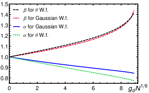
Figure 1: Comparison of the deformation of the cloud in momentum ($\alpha$) and position ($\beta$) spaces between Gaussian and $\theta$ -Wigner function (W.f.) for the $g_{d}$ in the stable regime. Notice very good agreement for stable range of $g_{d}N^{1/6}$.

The physics of two component gas is considerably richer than that of one component gas. First, the contact interaction between two different components is present. For Gaussian Wigner function (3) it has the form:

$$\vspace{-0em}E_{c}=g_{c}\frac{\lambda_{1}^{3/2}\lambda_{2}^{3/2}\sqrt{N_{1}N_{2}}\gamma^{-3}(2\pi)^{-3/2}}{\sqrt{\frac{\lambda_{1}}{\beta_{1}^{2}N_{1}^{1/3}}+\frac{\lambda_{2}}{\beta_{2}^{2}N_{2}^{1/3}}}\left(\frac{\lambda_{1}\beta_{1}}{N_{1}^{1/3}}+\frac{\lambda_{2}\beta_{2}}{N_{2}^{1/3}}\right)}.\vspace{-0.em}$$ (11)

It leads to the conventional Stoner transitionStoner (1947) and simultaneously stabilizes each component against deformations in momentum and position spaces.

Second, $V_{1221}$ is nonzero, so from Eq. (2) we see that in general terms like $f_{12}({\bf x},{\bf k})$ (called correlations between components) might appear. However, the ground state of an ideal gas is a product $\left|N_{1}\right\rangle\left|N_{2}\right\rangle$ so the intercomponent correlation function $\left\langle N_{1}\right|\left\langle N_{2}\right|\psi_{1}^{{}^{\dagger}}\psi_{2}\left|N_{1}\right\rangle\left|N_{2}\right\rangle$ vanishes and $f_{12}({\bf x},{\bf k})$ as well.

From a continuity argument for $f_{12}$ as a function of $g_{d}$ we can neglect for small $g_{d}$ the contribution of intercomponent correlations. Moreover, for unstable and fully magnetized ferronematic phase, properties of the system depend only on one component so correlations are not present. In further analysis we neglect correlations making the problem numerically tractable but paying the price of presenting more qualitative than quantitative results.

The third, dipolar energies for two components emerging from $V_{1212}$ and $V_{2121}$ have much more complicated form than for a single component. The direct energy between the two components is:

$$E_{dir}^{12}=-\frac{g_{d}N_{1}N_{2}}{2}\gamma^{-3}(2\pi)^{-3/2}\frac{g_{dip}(\kappa_{dir})}{\left(\frac{N_{1}^{1/3}}{\beta_{1}\lambda_{1}}+\frac{N_{2}^{1/3}}{\beta_{2}\lambda_{2}}\right)^{3/2}},$$ (12)

where: $\kappa_{dir}={(\frac{N_{1}^{1/3}\beta_{1}^{2}}{\lambda_{1}}+\frac{N_{2}^{1/3}\beta_{2}^{2}}{\lambda_{2}})}/{(\frac{N_{1}^{1/3}}{\beta_{1}\lambda_{1}}+\frac{N_{2}^{1/3}}{\beta_{2}\lambda_{2}})}.$ While the exchange energy between the two components is equal to:

$$E_{ex}^{12} = \frac{\frac{1}{2}g_{d}\gamma^{-3}(2\pi)^{-3/2}}{\sqrt{\frac{\lambda_{1}}{\beta_{1}^{2}N_{1}^{1/3}}+\frac{\lambda_{2}}{\beta_{2}^{2}N_{2}^{1/3}}}\sqrt{\frac{\alpha_{1}^{2}}{\lambda_{1}N_{1}^{1/3}}+\frac{\alpha_{2}^{2}}{\lambda_{2}N_{2}^{1/3}}}}$$ (13)

$$\times \frac{(\alpha_{1}\lambda_{1}N_{1}^{1/3}+\alpha_{2}\lambda_{2}N_{2}^{1/3})^{3/2}g_{dip}({\kappa_{ex}})}{\left(\frac{\beta_{1}\lambda_{1}}{N_{1}^{1/3}}+\frac{\beta_{2}\lambda_{2}}{N_{2}^{1/3}}\right)\times\left(\frac{1}{\alpha_{1}\lambda_{1}N_{1}^{1/3}}+\frac{1}{\alpha_{2}\lambda_{2}N_{2}^{1/3}}\right)},$$

where $\kappa_{ex}={(\alpha_{1}\lambda_{1}N_{1}^{1/3}+\alpha_{2}\lambda_{2}N_{2}^{1/3})}/{(\frac{\lambda_{1}N_{1}^{1/3}}{\alpha_{1}^{2}}+\frac{\lambda_{2}N_{2}^{1/3}}{\alpha_{2}^{2}})}.$ For the derivation see Supplemental material. The total energy is equal to

$$E^{1}_{kin}+E^{1}_{pot}+E^{2}_{kin}+E^{2}_{pot}+2(E_{dir}^{12}+E_{ex}^{12})+$$

$$+E^{1}_{dir}+E^{1}_{ex}+E^{2}_{dir}+E^{2}_{ex}+E_{c},$$ (14)

where single indexes $1$ or $2$ denotes component for which we take the kinetic, trap, direct and exchange energies, Eq. (5), (6), (7) and (8) accordingly .

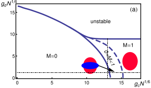
Figure 2: (a) Phase diagram for two component gas. Three regimes of different magnetization are visible. For $M=0$ size and shape of components are like for noninteracting gas. For $0<M<1$ Fermi surface of bigger component has the prolate shape (red) whereas for smaller one the oblate (blue). Thick, dashed line presents smooth crossover to the phase with $M=1$ where shape of the Fermi surface is prolate. The transition to the unstable regime is possible from ferronematic but also from unmagnetized phase. (b-c) Deformations in momentum and position spaces ($\alpha_{i}$ and $\beta_{i}$) as well as compression in the position space ($\lambda_{i}$) for constant $g_{d}N^{-1/6}=1.2$ and $g_{c}N^{-1/6}=13$ respectively (dash-dotted lines in (a)). In paramagnetic phase, due to the contact interaction, both components are getting bigger in position space with growing $g_{c}$. In ferronematic regime smaller component (index 2) still gets bigger while for constant $g_{d}$ parameter $\lambda_{1}$ goes to 1 what means equal occupation of the position and momentum phase spaces. For constant $g_{c}$ we see that the collapse is due to the higher occupation of the momentum rather than position phase space.

Fig. 2 shows the magnetization ($M=|N_{1}-N_{2}|/N$) and the stability of the system as a function of the dipolar and the contact coupling constants. In the area of $M=0$ (paramagnetic phase) both components have the same spherical shape. In the area where $0<M<1$ we have a ferronematic phase with partial magnetization. Of course the ground state is doubly degenerate. Either component could be a dominant one. The Fermi surface for the component with a higher occupation is prolate whereas for a lower occupation is oblate. For $M=1$ only one component is occupied and the Fermi surface is prolate. The unstable phase has a boundary with ferronematic (first order phase transition) and unmagnetized phase whereas for gas in a box only the transition from ferronematic to unstable regime is possible Fregoso and Fradkin (2009). On the other hand, in the trap, no direct transition from paramagnetic to ferronematic phase with M=1 is possible. The phase transition from paramagnetic to ferronematic with $M\neq 1$ is of the second order. Moreover, the partially magnetized ferronematic phase is much larger than for the box and extends up to the unstable regime. Using $\pi$ polarized light it is possible, due to the quadratic dependence of the AC Stark on magnetic quantum number, to prepare a system of ¹⁶¹Dy atoms in two extreme $m_{1,2}=\pm\nicefrac{{21}}{{2}}$ states. In this case $N=10^{6}$ atoms and $\omega=2\pi\times 100$Hz corresponds to $g_{d}N^{1/6}\approx 1$ in Fig. 2. By tuning the number of atoms it is possible to investigate the large part of the phase diagram.

The above analysis (as well as other presented in the literature) assumes that external magnetic field ${\bf B}$ is so small that it can be neglected. But in real cold atoms experiment the magnetic field may be controlled up to $10\mu G$ Pasquiou et al. (2011). One might ask a question what impact on the phase diagram has the ${\bf B}$ field?

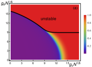
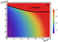
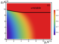
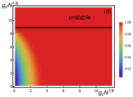
Figure 3: (a-d) Phase diagrams showing magnetization and unstable regime for several values of $g_{B}N^{-1/3}$ 0.0014, 0.14, 0.28 and 0.56 respectively. For nonzero magnetic field we no longer have paramagnetic phase. Black solid line shows the range of the unstable regime. Notice that the boundary between unstable and fully polarized ferronematic phase does not depend on the strength of magnetic field. For $N=10^{6}$ and $\omega=2\pi\times 100$Hz diagrams correspond to $B=0.01,1,2,4$ mG.

In the presence of a homogeneous magnetic field, the energy functional (2) is changed by addition of the term: $-g_{B}(N_{1}-N_{2})$, where we defined $g_{B}$ as equal to $\mu B$ and used the fact that the magnetic field is parallel to a quantization axis of the spin-$\nicefrac{{1}}{{2}}$. Results for different $g_{B}N^{-1/3}$ are presented in Fig. 3. For nonzero magnetic field we no longer have a paramagnetic phase and magnetization of the system continuously changes with $g_{d}$ and $g_{c}$. For the noninteracting gas we had spherical Fermi surfaces. They get more and more prolate ($1$st component) and oblate ($2$nd) with growing dipolar interaction up to the unstable phase. Of course now, the magnetic field favors the component with magnetic moment parallel to the magnetic field. Black solid line shows the range of the unstable regime. Notice that boundary between the unstable and fully polarized ferronematic phases does not depend on the strength of the magnetic field. Moreover, values of the magnetization for $g_{B}N^{-1/3}=0$ and $g_{B}N^{-1/3}=0.0014$ differ by less than 5%.

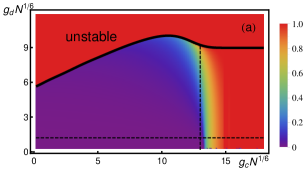
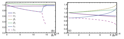
Figure 4: (a) Diagram showing $\frac{N_{1}-N_{2}}{N}$ for two component gas of $m_{1}=\nicefrac{{21}}{{2}}$ and $m_{2}=\nicefrac{{19}}{{2}}$ for different number of atoms and $\omega=2\pi\times 100$Hz. (b-c) Deformations in momentum and position spaces ($\alpha_{i}$ and $\beta_{i}$) as well as compression in the position space ($\lambda_{i}$) for constant $g_{d}N^{-1/6}=1.2$ and $g_{c}N^{-1/6}=13$ respectively (dashed lines in (a)). In whole range $N_{1}>N_{2}$ and both components, whenever exist, are prolate in momentum and position spaces (more elongated is the first one). The boundary of the stability of two components against collapse is strongly changed due to the interplay between contact and dipolar interactions.

The highest possible magnetic moment from all elements of ¹⁶¹Dy (10$\mu_{B}$) Lu et al. (2012) can be exploited in one more interesting system, namely in two component gas of $m_{1}=\nicefrac{{21}}{{2}}$ and $m_{2}=\nicefrac{{19}}{{2}}$. Using the magnetic quantum number dependent AC Stark shift and the Zeeman shift it can be prepared in a degenerate state (without dipolar interaction). The energy functional in analogy to Eq. (14) has the form: $E^{1}_{kin}+E^{1}_{pot}+E^{2}_{kin}+E^{2}_{pot}+E_{c}-2\frac{19}{21}(E_{dir}^{12}+E_{ex}^{12})+E^{1}_{dir}+E^{1}_{ex}+(\frac{19}{21})^{2}(E^{2}_{dir}+E^{2}_{ex})$ what comes from replacing Pauli matrix $\sigma_{z}$ in Eq. (1) by the matrix $\begin{pmatrix}1&0\\ 0&19/21\end{pmatrix}$. A corresponding phase diagram is presented in Fig. 4. Whereas in the case of $m_{1}=-m_{2}$ components we had large area of $N_{1}=N_{2}$ for this system we have $N_{1}>N_{2}$ for $g_{d}>0$ because the dipolar interaction is stronger for the 1st component. Both components are prolate in momentum and position spaces but the deformation is larger for the 1st one. The instability boundary of a one component gas is the same as for $m_{1}=m_{2}$ because it depends only on the larger magnetic moment. The most fascinating result is a nontrivial direct transition from the two component to an unstable system. Due to the interplay between the dipolar and contact interactions the last one is stabilizing the system more up to some critical value of $g_{c}N^{1/6}$.

In conclusion we have presented the first study of the ground state of the two component fermionic gas in a harmonic potential with dipolar and contact interactions. To be specific we have chosen parameters for the fermionic isotope ¹⁶¹Dy in the $m_{1,2}=\pm\nicefrac{{21}}{{2}}$ state where we have identified regimes of unstable, paramagnetic and ferronematic phases and transitions between them. We also showed that experimentally accessible control over the magnetic field enables observation of the sharp transition between the phases. Moreover, for ¹⁶¹Dy with $m_{1}=\nicefrac{{21}}{{2}}$, $m_{2}=\nicefrac{{19}}{{2}}$ we presented a nontrivial stability range due to the interplay between interactions. The generalization of our method may be adapted to other multicomponent phenomena in dipolar fermionic systems e.g the Einstein de-Haas effect or the spontaneous demagnetization.

Appendix A Derivation of direct and exchange energy between two components

The direct energy in (2) between two components without correlations has the form:

$$E_{dir}^{12}=\frac{1}{2(2\pi)^{6}}\int\!\mathrm{d}^{3}{\bf x}\,\int\!\mathrm{d}^{3}{\bf k}\,\int\!\mathrm{d}^{3}{\bf x}^{\prime}{}\,\int\!\mathrm{d}^{3}{\bf k}^{\prime}{}\,$$

$$\times f_{11}({\bf x},{\bf k})f_{22}({\bf x}^{\prime}{})V_{1122}({\bf x}-{\bf x}^{\prime}{}).$$

which after applying (4) can be writen as:

$$\vspace{-0em}E_{dir}^{12}=\frac{1}{2}\int\!\mathrm{d}^{3}{\bf x}\,\int\!\mathrm{d}^{3}{\bf x}^{\prime}{}\,n_{11}({\bf x},{\bf k})n_{12}({\bf x}^{\prime}{})V_{1122}({\bf x}-{\bf x}^{\prime}{}).\vspace{-0.em}$$

Using Fourier transform of the densities in position space:

$$\vspace{-0em}\mathcal{F}\{n_{ii}\}({\bf k})=N_{i}\exp\left[-\frac{k_{x}^{2}+k_{y}^{2}}{2\beta_{i}\lambda_{i}\gamma^{2}}N_{i}^{1/3}-\frac{\beta_{i}^{2}k_{z}^{2}}{2\lambda_{i}\gamma^{2}}N_{i}^{1/3}\right]\vspace{-0.em}$$

we get:

$$\vspace{-0em}E_{dir}^{12}=\frac{1}{2(2\pi)^{3}}\int\!\mathrm{d}^{3}k\,\mathcal{F}\{n_{11}\}({\bf k})\mathcal{F}\{V_{1122}\}({\bf k})\mathcal{F}\{n_{22}\}({\bf k}),\vspace{-0.em}$$

where the Fourier transform of the two body interaction is

$$\vspace{-0em}\mathcal{F}\{V_{1212}\}({\bf k})=-g_{d}(1-3\cos^{2}\theta).\vspace{-0.em}$$

The $k$-integration is then performed in spherical coordinates. After substitution of $\cos\theta$ by $u$ and performing integrals over $k$ and $\phi$ we get (12). The exchange energy between two components from (2) has the form:

$$E_{ex}^{12}=-\frac{1}{2(2\pi)^{6}}\int\!\mathrm{d}^{3}{\bf R}\,\int\!\mathrm{d}^{3}{\bf k}_{1}\,\int\!\mathrm{d}^{3}{\bf k}_{2}\,f_{11}({\bf R},{\bf k}_{1})$$

$$\times f_{22}({\bf R},{\bf k}_{2})\mathcal{F}\{V_{1122}\}({\bf k}_{1}-{\bf k}_{2}).$$

After performming substitutions: ${\bf k}={\bf k}_{1}-{\bf k}_{2}$ and ${\bf K}=\frac{{\bf k}_{1}+{\bf k}_{2}}{2}$ we get:

$$E_{ex}^{12}=-\frac{1}{2(2\pi)^{6}}\int\!\mathrm{d}^{3}{\bf R}\,\int\!\mathrm{d}^{3}{\bf k}\,\int\!\mathrm{d}^{3}{\bf K}\,f_{11}({\bf R},{\bf K}+\frac{{\bf k}}{2})$$

$$\times f_{22}({\bf R},{\bf K}-\frac{{\bf k}}{2})\mathcal{F}\{V_{1122}\}({\bf k}).$$

We see from the form of the $f_{ii}$ Eq. (3) that integral over ${\bf R}$ can be performed independently as a Gaussian integral. While $\mathcal{F}\{V_{1212}\}({\bf k})$ does not depend on ${\bf K}$. Next we can easily calculate the Gaussian integral over ${\bf K}$ in Cartesian coordinates. Finally, we transform the expression to spherical coordinates and after substituting $\cos\theta$ by $u$ we get Eq. (13).

Appendix B Multicomponent noninteracting gas

For multicomponent fermionic gas without dipolar and contact interaction in external ${\bf B}$ field calculus of variation can be used to find out distribution of atoms between components and the shapes in momentum and position spaces. The energy functional can be written using densities:

$$\sum_{m}\bigg{[}\int\!\mathrm{d}^{3}x\,\frac{3\hbar^{2}}{10M}(6\pi)^{2/3}{n_{m}({\bf x})^{5/3}}+\frac{M\omega^{2}x^{2}}{2}n_{m}({\bf x})$$

$$-\Gamma n_{m}({\bf x})-{\mu_{m}}Bn_{m}({\bf x})\bigg{]},$$

where $\Gamma$ is a Lagrange multiplier and we sum over components $m$.

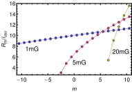
(a) size in position space of each component

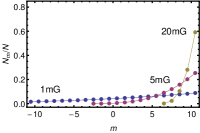
(b) number of atoms in each component

Figure 5: Size of the cloud and number of particles in every component for different magnetic fields. Results are for experimental parameters of $Dy$: $\mu=10\mu_{B}$, $\omega=2\pi\times 100Hz$ and $N=10^{6}$.

Next, we vary the energy functional with respect to densities $n_{m}({\bf x})$ getting for every $m$ the equation:

$$\frac{5}{3}\frac{3\hbar^{2}}{10M}(6\pi)^{2/3}{n_{m}({\bf x})^{2/3}}+M\omega^{2}r^{2}/2-\Gamma-{\mu_{m}}B=0,$$

from which we can find the distribution in position space for every $m$ as a function of $\Gamma$:

$$\vspace{-0em}n_{m}({\bf x})=\frac{(2M)^{3/2}}{6\pi^{2}\hbar^{3}}[\Gamma+\mu_{m}B-M\omega^{2}x^{2}/2]^{3/2}.\vspace{-0.em}$$

From the constraint on the total number of particles

$$N=\sum_{m}\int\!\mathrm{d}^{3}x\,{n_{m}({\bf x})}=\sum_{m}\frac{M^{3/2}(\Gamma+\mu_{m}B)^{3}}{3\left(M\omega^{2}\right)^{3/2}\hbar^{3}},$$

we find $\Gamma$. Once we have $\Gamma$ we can calculate the number of atoms in every component and the size of the components in position space $R_{m}$ (radius for which $n(R_{m})=0$).

Experimentally relevant ¹⁶¹Dy has magnetic dipole moment $\mu=10\mu_{B}$ with 22 hyperfine levels with $m_{F}\in\{-21/2,\dots,21/2\}$ and corresponding to it $\mu_{m}=\frac{20}{21}m_{F}\mu_{B}$.

Fig. 5 presents the size of components of ¹⁶¹Dy as a function of $m_{F}$ for different values of the ${\bf B}$ and $\omega=2\pi\times 100$Hz and $N=10^{6}$. The precision of ${\bf B}$ field control (up to $10\mu G$ Pasquiou et al. (2011)) is high enough to observe a true multicomponent ground state of the fermionic system with free magnetization in analogy to experiment with bosonic Cr Pasquiou et al. (2011). Such a thermalization to multicomponent state is not possible in the system with only contact interaction.