Time-shift invariance determines the functional shape of the current in dissipative rocking ratchets
Abstract
Ratchets are devices able to rectify an otherwise oscillatory behavior by exploiting an asymmetry of the system. In rocking ratchets the asymmetry is induced through a proper choice of external forces and modulations of nonlinear symmetric potentials. The ratchet currents thus obtained in systems as different as semiconductors, Josephson junctions, optical lattices, or ferrofluids, show a set of universal features. A satisfactory explanation for them has challenged theorist for decades, and so far we still lack a general theory of this phenomenon. Here we provide such a theory by exploring —through functional analysis— the constraints that the simple assumption of time-shift invariance of the ratchet current imposes on its dependence on the external drivings. Because the derivation is based on so general a principle, the resulting expression is valid irrespective of the details and the nature of the physical systems to which it is applied, and of whether they are classical, quantum, or stochastic. The theory also explains deviations observed from universality under special conditions, and allows us to make predictions of phenomena not yet observed in any experiment or simulation.
pacs:
05.60.-k, 05.45.Yv, 05.60.Cd, 02.30.SaI Introduction
Forcing nonlinear transport systems with zero-average, time-periodic, external forces may generate a ratchet current Cole et al. (2006). Ratchets are devices that exploit an asymmetry of the system (usually spatial) to rectify an otherwise oscillatory behavior Zapata et al. (1996); Falo et al. (1999); Linke et al. (1999); Villegas et al. (2003); Beck et al. (2005); Falo et al. (2002); Costache and Valenzuela (2010). The so-called rocking ratchets Reimann (2002); Hänggi and Marchesoni (2009) are able to do so by breaking a temporal symmetry —the external force cannot be reversed by a time shift— either in spatially symmetric systems Ajdari et al. (1994) or in the presence of some spatial asymmetry (see e.g. Refs. Reimann (2002); Astumian and Hänggi ). Ratchet currents can also be generated by a combined temporal and spatial symmetry breaking Poletti et al. (2008); Salger et al. (2009).
The two most studied mechanisms to induce a net current in a rocking ratchet are harmonic mixing Reimann (2002); Hänggi and Marchesoni (2009) and gating Tarlie and Astumian (1998); Zamora-Sillero et al. (2006); Gommers et al. (2008). In both of them the involved periodic spatial potentials are symmetric. Harmonic mixing amounts to imposing biharmonic external forces —typically with a frequency ratio 2:1— and has been experimentally observed Schneider and Seeger (1966); Seeger and Maurer (1978); Schiavoni et al. (2003); Ustinov et al. (2004); Gommers et al. (2005a); Ooi et al. (2007); Cubero et al. (2010) and theoretically studied Marchesoni (1986); Goychuk and Hänggi (1998); Flach et al. (2000); Morales-Molina et al. (2003) in many different physical systems, both classical and quantum. Biharmonic forces have also been used in experiments to modulate the potential in some thermal ratchets devices Engel et al. (2003); Jäger and Klapp (2012). In addition, harmonic mixing with more than two harmonics has been explored in experiments with optical lattices Gommers et al. (2006, 2007).
Gating ratchets also need at least two harmonics to break the temporal symmetry, but they play a different role Zamora-Sillero et al. (2006); Gommers et al. (2008); Noblin et al. (2009). In the most studied setup one of the two harmonics acts as an external force whereas the other one is used to modulate the spatial potential Zamora-Sillero et al. (2006); Gommers et al. (2008).
Currents generated through many different rocking ratchets share a few properties that hold regardless of the system. When two harmonics are used and their amplitudes are small, the current exhibits a shifted sinusoidal shape as a function of a precise combination of the phases of both harmonics. This has been experimentally observed in semiconductors Schneider and Seeger (1966), optical lattices Schiavoni et al. (2003), ferrofluids Engel et al. (2003), and Josephson junctions Ustinov et al. (2004); Ooi et al. (2007) and has been theoretically confirmed in studies of transport in semiconductors Schneider and Seeger (1966), Brownian particles Marchesoni (1986); Wonneberger (1979), solitons Zamora-Sillero et al. (2006); Salerno and Zolotaryuk (2002); Morales-Molina et al. (2003), ferrofluids Engel et al. (2003), and magnetic particles via dipolar interactions Jäger and Klapp (2012), among other systems. The phase lag of the sinusoid is known to depend on the frequency of the harmonics, the damping, and other specific parameters of the system Breymayer (1984); Borromeo et al. (2005) —accordingly, current reversals can be induced by acting on these parameters. Moreover, the ratchet current is always found to be proportional to a product of specific powers of the amplitudes of the harmonics.
Upon increasing the amplitudes of the harmonics beyond the small limit regime departures from the sinusoidal behavior are observed, both in experiments Noblin et al. (2009) and simulations Cubero et al. (2010). As a consequence, current reversals can also be induced by tuning the amplitudes of the harmonics Reimann (2002); Goychuk and Hänggi (1998).
Although there have been many theoretical attempts to explain these universal features of rocking ratchets, their scope is very limited, constrained to specific models, and only applied to harmonic mixing. For instance, stochastic theories have been used to explain the Brownian motion of a charged particle in a periodic symmetric potential driven with a biharmonic force Wonneberger (1979); Breymayer (1984). Also, collective coordinate theories have successfully explained harmonic mixing Salerno and Zolotaryuk (2002); Morales-Molina et al. (2003) and gating Zamora-Sillero et al. (2006) in soliton ratchets. For several models described by nonlinear differential equations, symmetry properties of the current and of the systems can only provide conditions on the two harmonics for a ratchet current to exist Reimann (2002); Ajdari et al. (1994); Zamora-Sillero et al. (2006); Flach et al. (2000).
For decades, all attempts to reproduce the sinusoidal shape of the current have failed to predict the existence of a system-dependent phase lag. This lack of success is due to a flawed assumption —widely employed in the literature under the name of moment method— upon which all these theories rely. According to this method, the ratchet current can be obtained as an expansion in odd moments of the external force (starting at the third moment because the time-average of the force is zero by construction). That this method is generally incorrect has been shown in Ref. Quintero et al. (2010) —where the very restricted conditions for its validity were properly delimited— but it is easy to see why in an example: If the force is a square wave all, its powers are proportional to the force itself, and therefore the current must be zero. That this is not the case has been shown in experiments Arzola et al. (2011), simulations Ajdari et al. (1994); Schreier et al. (1998), and also theoretically in Ref. Quintero et al. (2011). The application of this method apparently captures the right dependence on the amplitudes in the case of harmonic mixing, but this is purely accidental. (For an in-depth analysis of this method and its many flaws, see Refs. Quintero et al. (2010, 2011) and references therein.)
An alternative theoretical approach has been recently proposed for the case of harmonic mixing Quintero et al. (2010). This theory does capture the nonzero phase lag that the ratchet current normally exhibits and also predicts a nonzero current for square-wave forces Quintero et al. (2011). Nevertheless, despite this relative success, a general theory that encompasses a unified explanation of all universal features observed in so wide a diversity of systems, an explanation of the deviations from them that occur outside the small-amplitude regime and the effects induced by further harmonics, is still lacking. Such a theory cannot be based on the particulars of specific systems but has to rely on very general principles that hold for all of them.
In this paper, we explore the constraints that the simple time-shift invariance satisfied by the ratchet current imposes on its shape and derive an expression that explains all observations described above, both for harmonic mixing and gating ratchets (with any number of harmonics). The formula describes correctly not only the small-amplitude regime but also the deviations found for larger amplitudes. And, because it is based on so general a principle, it is valid regardless of the (dissipative) system and applicable even in the absence of a mathematical model describing the phenomenon Noblin et al. (2009). On top of that, it allows us to make predictions so far not observed in any experiment or simulation.
Before we enter into the details, a remark seems appropriate about what this theory is not. This theory is not meant to predict when a system does exhibit a ratchet phenomenon. This is not possible because the theory is so general that it holds both for dissipative systems that do and that do not have ratchet currents. What the theory provides is a pattern to which any ratchet current must conform. The theory claims that, under certain regularity conditions, the ratchet current —if any— must necessarily be of a given specific form. But the pattern depends on a set of unknown, system specific coefficients that might all be zero —hence yielding a zero current. For the same reason the theory cannot predict any effect that depends on specific details of the system. Having clarified this, what the theory does predict is that the current must necessarily be zero if the system possesses some specific symmetries —so it is consistent with the well known fact that, unless some symmetries are broken, a ratchet current cannot be generated Ajdari et al. (1994); Flach et al. (2000); Reimann (2002).
II General theory
Suppose we have a physical system describing the position of a particle or localized structure, , as a function of time. The system is driven by some periodic, time-dependent, external driving (external force, parameter modulation, etc.). Function —or its expectation if the system is stochastic— is uniquely determined for any given , and so is the ratchet current defined as
| (1) |
Mathematically this means that the current is a functional of the external driving . Except for very specific systems in which also depends on the initial conditions (e.g., Hamiltonian systems or other nondissipative systems Salger et al. (2009)), will —by construction— be invariant under time shifts. We will show that the fact that is a time-invariant functional of is enough to determine the shape of the ratchet current for specific drivings regardless of the system under study, as long as some regularity assumptions of this functional dependence hold. Moreover, new symmetries of the system can be incorporated into the theory to further specify this shape.
II.1 Time-shift-invariant functionals of periodic functions
Let , with , be the set of continuous, -periodic functions , and let be a real functional on . If is times Fréchet differentiable on , then it has an -th order Taylor expansion around Wouk (1979). Such a Taylor expansion can be obtained as the -th order truncation of the series 111In Eq. (2), it is implicitly assumed that if for some , variables and factors are missing; e.g., for and , the terms within the angular brackets are . With the same convention, is just a constant.
| (2) |
where and we have introduced the notation
| (3) |
The kernels are all real, -periodic, and symmetric in all their arguments.
In order to avoid cumbersome expressions we will henceforth work with the full series (2). It goes without saying that if is at most times Fréchet differentiable the results we will obtain still hold if the series are truncated at th-order and an appropriate error term is added Wouk (1979).
Consider the time-shift operator . We will say that is invariant under time shift if for all . Time-shift invariance reflects on the kernels in Eq. (2) as the property
| (4) |
for all .
Theorem 1.
Let be a time-shift-invariant functional with Taylor series (2), and take
| (5) |
where is such that 222 stands for “greatest common divisor” of , i.e., the largest integer that divides all . and . Let denote the set of nonzero solutions of the Diophantine equation 333The term Diophantine equation refers to an equation involving only integer numbers. It is named after Diophantus of Alexandria, who introduced them in his treatise Arithmetica. , whose leftmost nonzero component is positive. Then,
| (6) |
where , , and functions and do not depend on and are even in each , , for every .
(The proof of this theorem is deferred to Appendix A.)
When the functional exhibits further symmetries, some of the unknown functions and in the expansion (6) can be determined. Two symmetries are important in this respect: force-reversal and time-reversal.
Definition 1 (Force reversal).
Let be a nonempty subset of indexes and let . We define the force-reversal operation on as the new vector function such that if and if .
Corollary 1.
Under the conditions of Theorem 1, let (). Then, if and only if for all such that is even.
Since is even in all its arguments, this simply follows by replacing in Eq. (6) by for all .
Definition 2 (Time reversal).
Let . We define the time-reversal operation on as .
Corollary 2.
Under the conditions of Theorem 1,
-
(a)
if and only if for each and
-
(b)
if and only if or for each .
The proof of this corollary follows upon realizing that time-reversal amounts to replacing by , for all , in (6).
III Application to different systems
Equation (6) has been derived under the assumption that is a sufficiently regular functional of and that it is time-shift invariant. Because these two assumptions are so general, it turns out that the functional form (6) must hold regardless of the specific system to which it is applied. In particular, details such as the kind of nonlinearities, whether we deal with a particle or a localized field, the actual parameters, etc., can only modify the functions and , and only in a very specific way (they must be even functions of the amplitudes ). Furthermore, had the system one of the symmetries of Corollaries 1 and 2, some of these functions would get automatically fixed regardless of any other particular. This renders Eq. (6) a universal expansion for the currents of rocking ratchets. In what follows, we discuss its application to explain different experimental and numerical results reported in the literature of rocking ratchets.
III.1 Two harmonic forces
We start by considering systems for which the ratchet current arises from the combined effect of two harmonics, and . This special case is of great importance because most rocking ratchets are induced by a biharmonic force Schiavoni et al. (2003); Ustinov et al. (2004); Gommers et al. (2005a); Ooi et al. (2007); Cubero et al. (2010); Marchesoni (1986); Goychuk and Hänggi (1998); Flach et al. (2000); Morales-Molina et al. (2003); Engel et al. (2003). But it also comprises the so-called gating ratchets Hänggi and Marchesoni (2009); Zamora-Sillero et al. (2006); Gommers et al. (2008), for which is an external force whereas modulates the amplitude of a nonlinear potential.
For two harmonics, the Diophantine equation becomes . Its solutions are given by , , but those contributing to (6) have . Therefore , and (6) reads
| (7) |
with .
Although Eq. (7) is valid for both, ratchets induced by a biharmonic force and gating ratchets, their differences arise from their different force-reversal symmetries. Let us analyze both cases separately.
III.2 Ratchets induced by a biharmonic force
In rocking ratchets with symmetric spatial potentials the current gets reversed upon reversing the force (see, e.g., Ref. Reimann (2002); Hänggi and Marchesoni (2009); Quintero et al. (2010) and references therein). Formally . Since either and are both odd or have a different parity. In the former case is always even, so according to Corollary 1, for all and therefore (i.e., there is no ratchet current). Notice that in this case , and since is time-shift invariant but changes sign under force reversal, it can only be . This explains our finding.
On the contrary, if is odd [in which case for all ], then Corollary 1 implies only , ; hence
| (8) |
The lowest order in Eq. (8) yields
| (9) |
a result first obtained in Eq. Quintero et al. (2010).
But, Eq. (8) contains more information. The lowest order at which the next harmonic enters in is . For the simplest —and most common— case studied in the literature, namely, and , this implies that the second harmonic first appears at ninth order. Therefore, an improvement on Eq. (9) is
| (10) |
where the error contains terms of order 9 or higher, and and are quadratic polynomials in and . Equation (10) tells us that, whereas Eq. (9) captures the shape of the ratchet current for sufficiently small amplitudes, upon increasing the amplitudes we can modify the phase lag . Put in a different way, if we fix the phases and of the biharmonic force so that , the ratchet current is suppressed Gommers et al. (2005a); Borromeo et al. (2005). But then we can restore it without changing the phases by increasing the amplitudes.
This current reversal was observed in experiments Gommers et al. (2005a); Cubero et al. (2010) and attributed to a dissipation-induced symmetry breaking. Our Eq. (10) reveals that this is the default behavior of a ratchet like this, because the current vanishes at a value of that depends not only on the amplitudes of the biharmonic force, but also on the frequency and other parameters of the system.
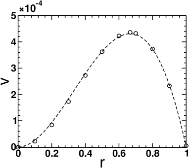
Functions and are experimentally obtained for a range of values of Cubero et al. (2010). Figure 1 shows a fit of the experimental data to the curve , with being and quadratic polynomials in .
Another prediction of the theory follows from Corollary 2: For systems having either of those two symmetries upon time reversal, all phase lags in the expansion (8) are constant —either or , or , depending on the symmetry. This is confirmed, e.g., by simulations carried out on the Langevin equation
| (11) |
with a zero-mean white noise such that and is a biharmonic force Cubero et al. (2010). Figure 4 (upper panel) of Ref. Cubero et al. (2010) shows that for all amplitudes. (In this overdamped regime, the velocity does not change sign upon time reversal.) This figure is especially revealing because for the largest amplitudes, the velocity clearly shows the influence of the second harmonic, and yet the phase lags remain constant.
III.3 Gating ratchets
Force reversal acts differently for gating ratchets because, of the two harmonics, only is an external force. In this case, when the potential is symmetric Hänggi and Marchesoni (2009); Zamora-Sillero et al. (2006); Gommers et al. (2008), we have . Thus, Corollary 1 implies if is even (). If is even, then , whereas if is odd, then only , , and we again recover Eqs. (8) and (9). Notice that if is even, then must be odd [because ], and therefore and . Thus, a time shift can reverse the current —which means that the current must be zero.
Thus, the ratchet currents produced by either gating or a biharmonic force are both given by the same formula. There is an exception, though: Gating does not put any constraint on , so a ratchet current can be obtained even for Hänggi and Marchesoni (2009); Zamora-Sillero et al. (2006); Gommers et al. (2008). For this particular case, the lowest order at which the second harmonic shows up in the current is the sixth, i.e.,
| (12) |
and and are linear in and . Accordingly, a shift of the phase lag with the amplitudes similar to that observed in biharmonic ratchets Cubero et al. (2010) is to be expected in gating ratchets. Thus, not only has formula (12) been obtained here for the first time (to the best of our knowledge, no theory has ever been attempted to explain the current observed in gating ratchets) but the possibility of inverting the current by varying the amplitudes of the harmonics in these systems is a prediction of this theory that, as far as we know, still needs experimental confirmation.
III.4 Particles moving in asymmetric potentials
An interesting case to analyze with the theory is that of particles moving (or solitons lying) in potentials lacking mirror symmetry. In these cases, the current does not have the force-reversal symmetry exploited above because the mirror image of the system is a different system. Then, all terms in (7) are nonzero in principle. In the case of two harmonics —irrespective of whether we are considering ratchets induced by biharmonic forces or gating ratchets— the lowest order in the expansion (7) is given by , a polynomial of and . Clearly, if there is no ratchet current in the absence of external force; therefore, in this case, the theory predicts, for small amplitudes, a ratchet current independent of the phases (a dependence that may be restored at higher orders) and proportional to a linear combination of and .
As a matter of fact, the theory also predicts that even with a single harmonic (say, ), a ratchet current proportional to can be generated. This is indeed what was found in Refs. Reimann (2002); Quintero et al. (2005). In this case we also know from Eq. (7) that all higher-order terms are identically zero, so the prediction is even stronger: The current must be of the form , with a certain function. Notice in particular that, depending on whether does or does not change sign, the current may or may not exhibit reversals upon variations of the amplitude .
III.5 Other ratchets with two harmonics
Liquid drops on a horizontal plate exhibit ratchet movement when the plate is vibrated with both horizontal and vertical harmonic forces Noblin et al. (2009). These forces have the same frequency and a relative phase , and as usual the ratchet current depends on . We are not aware of any theoretical approach that explains why the average velocity of the drops exhibits a nonsinusoidal behavior as a function of the relative phase shift . However, Fig. 3(a) of Ref. Noblin et al. (2009) reveals that changes sign when the vertical force is reversed; i.e., . According to our approach, this is enough to conclude that the drop velocity must behave as the current of a gating ratchet. Hence, it will be given by Eq. (8) for . Figure III.5 shows a fit with the first two harmonics of this equation to the experimental data of Ref. Noblin et al. (2009).
This anharmonicity is also predicted by our theory when the ratchet is induced by a biharmonic force with large amplitudes, and it has been reported recently in simulations of classical particles in a one-dimensional driven superlattice Wulf et al. (2012).
![[Uncaptioned image]](/html/1308.0491/assets/x2.png)
captionDroplet velocity as function of the phase shift between the horizontal and vertical vibrations of the plate. Symbols represent experimental data from Figure 3, upper panel, , of Ref. Noblin et al. (2009). The line represents the fit of the curve .
III.6 Forcing with more than two harmonics
In some experiments with cold atoms Gommers et al. (2006, 2007), ratchets are generated using more than two harmonics. The simplest one is of the form
| (13) |
Although the Diophantine equation has three unknowns, the solution can be readily obtained using Blankinship’s algorithm Morito and Salkin (1980) as , where , , and . Hence, . The subset contributing to (6) is defined by ; on the other hand, because of force reversal (c.f. Corollary 1), the only nonzero coefficients have odd. Hence, if is even, then must be odd, whereas if is odd, then must be odd. Then,
| (14) |
where , , and if is even, or if is odd.
The choice Gommers et al. (2006) reduces Eq. (13) to a biharmonic force where the amplitude of the one of harmonics depends on the phase . In other words, the shape of the current is again a sinusoidal function of , with the usual cubic prefactor of the amplitudes; however, in this case both the maximum current and the phase lag depend on . This is exactly what the experiments reveal (c.f. Fig. 1 of Ref. Gommers et al. (2006)).
Another relevant choice of parameters is and Gommers et al. (2006). For , it implies that . Thus, regardless of the parity of , Eq. (14) becomes
| (15) |
The lowest order is , which explains the observations made in Ref. Gommers et al. (2006), namely, the sinusoidal dependence on and the insensitivity of to variations of the phase .
The limit case is particularly interesting because it connects the effect of perturbations with quasiperiodic forces. Suppose the harmonics depend on two frequencies, and , such that is not a rational number. One can choose rational approximants of such that and for a suitable . The theory can then be applied for each choice of and , and the quasiperiodic limit can be recovered as the limit and with . For an illustration of the application of this method, we refer to the appendix of Ref. Cubero and Renzoni (2012).
A second more complicated forcing has also been tested for cold atoms Gommers et al. (2007). The force in this case can be cast as a sum of four harmonics , where
| (16) |
Two cases have been studied Gommers et al. (2007): and , .
For , , and there are three harmonics left. The expansion of in terms of and the amplitudes can be obtained using a similar procedure [see Appendix B, Eq. (27)]. To lowest order,
| (17) |
where contains five-order terms in and . This expression features, even at the lowest order in the amplitudes, a deviation from the usual sinusoidal shape. In the experiments, the second harmonic went unnoticed because at that time no available theory predicted any such deviation. However, the fit of the experimental data to a cosine function shows a systematic discrepancy that might be the fingerprint of this second harmonic (c.f. Fig. 1 of Ref. Gommers et al. (2007)). Further experiments should reveal this second harmonic more clearly.
The second case experimentally tested is , . For this case, all four harmonics (16) are present. The full expansion in terms of and the amplitudes is obtained in Appendix B [c.f. Eq. (28)]. To lowest order,
| (18) |
with and given by (30).
The usual cosine shape of the current was already observed in the experiments Gommers et al. (2007). However, Eq. (18) reveals an unexpected new effect. In harmonic mixing currents, it is customary to set and and vary . If the system is driven by a biharmonic force, changing changes the intensity of the current Schiavoni et al. (2003). However, if is sufficiently small, the phase at which the current vanishes does not depend on . In other words, if is fixed to this phase and is varied, no ratchet current is produced. (As explained before [c.f. Eq. (10)], this is no longer true if is large; see also Ref. Cubero et al. (2010).) But Eq. (18) tells us that does depend on even for small . This implies that by setting so that the current is zero for a given , we can generate a ratchet current by simply changing .
To confirm this prediction of the theory we carry out simulations for the damped sine-Gordon equation
| (19) |
driven by the multifrequency force (16) with , . We have solved numerically this equation in the interval , with periodic boundary conditions, by discretizing the second spatial derivative using centered finite differences on a grid of step size . We have integrated the resulting set of ordinary differential equations with a fourth-order Runge-Kutta method along 10 complete periods, with a time step . As the initial condition, we use an exact static one-soliton solution, centered at zero, of the unforced [] and undamped () sine-Gordon equation (19).
Notice that if or , only two of the four harmonics (16) remain. Their frequencies are such that for , —hence, there is no ratchet current— whereas for this symmetry is broken —hence there is a ratchet current. Accordingly, we set and , and find the value of for which . Then, we fix this value for and vary . The result is shown in Fig. 2. As predicted, varying induces a ratchet current. As a matter of fact, the numerical values fit perfectly the theoretical prediction that follows from Eqs. (18) and (29).
IV Discussion and conclusions
In this work, we have introduced a theory that captures, in a unified framework, the ratchet transport generated by zero-average, periodic drivings of very different kinds of systems, like cold atoms in optical lattices, fluxons in Josephson junctions, current in semiconductors, or transport of ferromagnetic nanoparticles in liquids. The theory can be applied to classical or quantum dissipative systems alike, with or without thermal fluctuations. The number of different harmonics the theory can deal with is arbitrary. Although most studies use two, added up in a single biharmonic force or used for two different purposes (like a force and a potential modulation Zamora-Sillero et al. (2006); Gommers et al. (2008) or two independent forces Noblin et al. (2009)), the theory also explains experiments carried out driving the system with three or four harmonics Gommers et al. (2006, 2007), as well as experiments in ferrofluids, where the biharmonic force modulates the potential in a new type of thermal ratchet device Engel et al. (2003).
Focusing on the results for two harmonics, Eq. (7) already captures many universal features observed in experiments and simulations. First, it shows the widespread sinusoidal dependence observed when the amplitude of the external forces is small Schneider and Seeger (1966); Zamora-Sillero et al. (2006); Gommers et al. (2008); Schiavoni et al. (2003); Ustinov et al. (2004); Ooi et al. (2007); Goychuk and Hänggi (1998); Morales-Molina et al. (2003); Engel et al. (2003). Second, it explains why the sinusoid is observed even when the amplitude of the force is not so small Cubero et al. (2010). Third, it captures the departures of this sinusoidal shape for even larger amplitudes Cubero et al. (2010); Noblin et al. (2009). And fourth, it shows that the point where the current vanishes (the phase lag) depends on the amplitude, the frequency, and the rest of the system parameters. In particular, this means that we can generate or revert the current by simply changing the amplitudes of the two harmonics Cubero et al. (2010); Noblin et al. (2009), their frequency Breymayer (1984); Gommers et al. (2005b), or (rather paradoxically) the damping in systems with dissipation Gommers et al. (2005a); Breymayer (1984); Morales-Molina et al. (2006); Quintero et al. (2011). If the system satisfies certain symmetries, the theory predicts that the phase lags can no longer be modified by changing the amplitudes of the harmonics (Corollary 2). This is indeed what happens in some equations for particles or solitons moving in a nonlinear potential and in certain experiments Ooi et al. (2007); Marchesoni (1986); Engel et al. (2003); Quintero et al. (2011).
One of the most remarkable facts about this theory is its universality. In its derivation, we have simply used two assumptions: (a) The velocity is a sufficiently regular functional of the external force (regularity condition), and (b) it is invariant under time shifts (time-shift symmetry). The former is used to make a Taylor expansion —perhaps only up to some finite order— of the velocity with respect to the external force; the latter leads, in the case of harmonic forcings, to a Fourier expansion in terms of some combination of the phase shifts between the harmonics. The fact that the functional form (6) is obtained under so general assumptions implies that the particulars of the system under study (e.g., the kind of nonlinearities or the specific parameters) can only tune the constants but never change the functional form. As a matter of fact, we do not even need to have an explicit mathematical model of the experimental system to predict how the velocity depends on the phases of the harmonics and to constrain its dependence on the amplitudes (e.g., the case analyzed in Fig. III.5).
Of the two assumptions above, only regularity limits the applicability of the theory. Besides, it might be a requirement that is hard to verify for a given physical system. Nonetheless, the success of the theory in explaining the results of so many different experimental and numerical sources suggests that the systems to which it does not apply must be rare. Exceptions can be found, though. For instance, simulations of the discrete Frenkel-Kontorova system show discontinuities in the behavior of the current as a function of the phases in the biharmonic force Zolotaryuk and Salerno (2006). Also, the ratchet current of periodically forced overdamped particles moving in an asymmetric potential exhibits discontinuities as a function of the amplitude of the forcing Bartussek et al. (1994); Ajdari et al. (1994) —although these discontinuities disappear in the presence of noise, which may thus be acting as a regularizer of the functional.
We end by pointing out that universality permits us not only to explain a plethora of specific phenomena or anomalies that different experiments and simulations have evidenced but also to predict new ones that have not been observed yet and need experimental confirmation. Some of them are described above, and some others have been stated along the way while analyzing systems which had been experimentally studied. But, by making specific choices for the number of harmonics and their frequencies in Eq. (6), many more can be derived.
References
- Cole et al. (2006) D. Cole, S. Bending, S. Savel’ev, A. Grigorenko, T. Tamegai, and F. Nori, “Ratchet without spatial asymmetry for controlling the motion of magnetic flux quanta using time-asymmetric drives,” Nat. Mater. 5, 305–311 (2006).
- Zapata et al. (1996) I. Zapata, R. Bartussek, F. Sols, and P. Hänggi, “Voltage Rectification by a SQUID Ratchet,” Phys. Rev. Lett. 77, 2292–2295 (1996).
- Falo et al. (1999) F. Falo, P. J. Martínez, J. J. Mazo, and S. Cilla, “Ratchet potential for fluxons in Josephson-junction arrays,” Europhys. Lett. 45, 700–706 (1999).
- Linke et al. (1999) H. Linke, T. E. Humphrey, A. Lofgren, A. O. Sushkov, R. Newbury, R. P. Taylor, and P. Omling, “Experimental Tunneling Ratchets,” Science 286, 2314–2317 (1999).
- Villegas et al. (2003) J. E. Villegas, S. Savel’ev, F. Nori, E. M. González, J. V. Anguita, R. García, and J. L. Vicent, “A Superconducting Reversible Rectifier That Controls the Motion of Magnetic Flux Quanta,” Science 302, 1188–1191 (2003).
- Beck et al. (2005) M. Beck, E. Goldobin, M. Neuhaus, M. Siegel, R. Kleiner, and D. Koelle, “High-Efficiency Deterministic Josephson Vortex Ratchet,” Phys. Rev. Lett. 95, 090603 (2005).
- Falo et al. (2002) F. Falo, P. J. Martínez, J. J. Mazo, T. P. Orlando, K. Segall, and E. Trías, “Fluxon ratchet potentials in superconducting circuits,” Appl. Phys. A 75, 263–269 (2002).
- Costache and Valenzuela (2010) M. V. Costache and S. O. Valenzuela, “Experimental Spin Ratchet,” Science 330, 1645–1648 (2010).
- Reimann (2002) P. Reimann, “Brownian motors: noisy transport far from equilibrium,” Phys. Rep. 361, 57–265 (2002).
- Hänggi and Marchesoni (2009) P. Hänggi and F. Marchesoni, “Artificial Brownian motors: Controlling transport on the nanoscale,” Rev. Mod. Phys. 81, 387–442 (2009).
- Ajdari et al. (1994) A. Ajdari, D. Mukamel, L. Peliti, and J. Prost, “Rectified motion induced by ac forces in periodic structures,” J. Phys. I France 4, 1551–1561 (1994).
- (12) R. D. Astumian and P. Hänggi, “Brownian Motors,” Phys. Today 55.
- Poletti et al. (2008) D. Poletti, T. J. Alexander, E. A. Ostrovskaya, B. Li, and Yu. S. Kivshar, “Dynamics of Matter-Wave Solitons in a Ratchet Potential,” Phys. Rev. Lett. 101, 150403 (2008).
- Salger et al. (2009) T. Salger, S. Kling, T. Hecking, C. Geckeler, L. Morales-Molina, and M. Weitz, “Directed Transport of Atoms in a Hamiltonian Quantum Ratchet,” Science 326, 1241 (2009).
- Tarlie and Astumian (1998) M. B. Tarlie and R. D. Astumian, “Optimal modulation of a Brownian ratchet and enhanced sensitivity to a weak external force,” PNAS 95, 2039–2043 (1998).
- Zamora-Sillero et al. (2006) E. Zamora-Sillero, N. R. Quintero, and F. G. Mertens, “Ratchet effect in a damped sine-Gordon system with additive and parametric ac driving forces,” Phys. Rev. E 74, 046607 (2006).
- Gommers et al. (2008) R. Gommers, V. Lebedev, M. Brown, and F. Renzoni, “Gating Ratchet for Cold Atoms,” Phys. Rev. Lett. 100, 040603 (2008).
- Schneider and Seeger (1966) W. Schneider and K. Seeger, “Harmonic Mixing of Microwaves by Warm Electrons in Germanium,” Appl. Phys. Lett. 8, 133–135 (1966).
- Seeger and Maurer (1978) K. Seeger and V. Maurer, “Nonlinear Electronic Transport in TTF-TCNQ Observed by Microwave Harmonic Mixing,” Solid State Commun. 27, 603–606 (1978).
- Schiavoni et al. (2003) M. Schiavoni, L. Sánchez-Palencia, F. Renzoni, and G. Grynberg, “Phase Control of Directed Diffusion in a Symmetric Optical Lattice,” Phys. Rev. Lett. 90, 094101 (2003).
- Ustinov et al. (2004) A. V. Ustinov, C. Coqui, A. Kemp, Y. Zolotaryuk, and M. Salerno, “Ratchetlike Dynamics of Fluxons in Annular Josephson Junctions Driven by Biharmonic Microwave Fields,” Phys. Rev. Lett. 93, 087001 (2004).
- Gommers et al. (2005a) R. Gommers, S. Bergamini, and F. Renzoni, “Dissipation-Induced Symmetry Breaking in a Driven Optical Lattice,” Phys. Rev. Lett. 95, 073003 (2005a).
- Ooi et al. (2007) S. Ooi, S. Savel’ev, M. B. Gaifullin, T. Mochiku, K. Hirata, and F. Nori, “Nonlinear Nanodevices Using Magnetic Flux Quanta,” Phys. Rev. Lett. 99, 207003 (2007).
- Cubero et al. (2010) D. Cubero, V. Lebedev, and F. Renzoni, “Current reversals in a rocking ratchet: Dynamical versus symmetry-breaking mechanisms,” Phys. Rev. E 82, 041116 (2010).
- Marchesoni (1986) F. Marchesoni, “Harmonic mixing signal: Doubly dithered ring laser gyroscope,” Phys. Lett. A 119, 221–224 (1986).
- Goychuk and Hänggi (1998) I. Goychuk and P. Hänggi, “Quantum Rectifiers From Harmonic Mixing,” Europhys. Lett. 43, 503–509 (1998).
- Flach et al. (2000) S. Flach, O. Yevtushenko, and Y. Zolotaryuk, “Directed Current due to Broken Time-Space Symmetry,” Phys. Rev. Lett. 84, 2358–2361 (2000).
- Morales-Molina et al. (2003) L. Morales-Molina, N. R. Quintero, F. G. Mertens, and A. Sánchez, “Internal Mode Mechanism for Collective Energy Transport in Extended Systems,” Phys. Rev. Lett. 91, 234102 (2003).
- Engel et al. (2003) A. Engel, H. W. Müller, P. Reimann, and A. Jung, “Ferrofluids as Thermal Ratchets,” Phys. Rev. Lett. 91, 060602 (2003).
- Jäger and Klapp (2012) S. Jäger and S. H. L. Klapp, “Rotational ratchets with dipolar interactions,” Phys. Rev. E 86, 061402 (2012).
- Gommers et al. (2006) R. Gommers, S. Denisov, and F. Renzoni, “Quasiperiodically Driven Ratchets for Cold Atoms,” Phys. Rev. Lett. 96, 240604 (2006).
- Gommers et al. (2007) R. Gommers, M. Brown, and F. Renzoni, “Symmetry and transport in a cold atom ratchet with multifrequency driving,” Phys. Rev. A 75, 053406 (2007).
- Noblin et al. (2009) X. Noblin, R. Kofman, and F. Celestini, “Ratchetlike Motion of a Shaken Drop,” Phys. Rev. Lett. 102, 194504 (2009).
- Wonneberger (1979) W. Wonneberger, “Stochastic Theory of Harmonic Microwave Mixing in Periodic Potentials,” Solid State Commun. 30, 511–514 (1979).
- Salerno and Zolotaryuk (2002) M. Salerno and Y. Zolotaryuk, “Soliton ratchetlike dynamics by ac forces with harmonic mixing,” Phys. Rev. E 65, 056603 (2002).
- Breymayer (1984) H. J. Breymayer, “Harmonic Mixing in a Cosine Potential for Arbitrary Damping,” Appl. Phys. A 33, 1–7 (1984).
- Borromeo et al. (2005) M. Borromeo, P. Hänggi, and F. Marchesoni, “Transport by bi-harmonic drive: from harmonic to vibrational mixing,” J. Phys.: Condens. Matter 17, S3709–S3718 (2005).
- Quintero et al. (2010) N. R. Quintero, J. A. Cuesta, and R. Alvarez-Nodarse, “Symmetries shape the current in ratchets induced by a bi-harmonic drivig force,” Phys. Rev. E 81, 030102 (2010).
- Arzola et al. (2011) A. V. Arzola, K. Volke-Sepulveda, and J. L. Mateos, “Experimental Control of Transport and Current Reversals in a Deterministic Optical Rocking Ratchet,” Phys. Rev. Lett. 106, 168104 (2011).
- Schreier et al. (1998) M. Schreier, P. Reimann, P. Hänggi, and E. Pollak, “Giant enhancement of diffusion and particle selection in rocked periodic potentials,” Europhys. Lett. 44, 416–422 (1998).
- Quintero et al. (2011) N. R. Quintero, R. Alvarez-Nodarse, and J. A. Cuesta, “Ratchet effect on a relativistic particle driven by external forces,” J. Phys. A 44, 425205 (2011).
- Wouk (1979) A. Wouk, Course of Applied Functional Analysis (John Wiley & Sons, New York, 1979).
- Note (1) In Eq. (2\@@italiccorr), it is implicitly assumed that if for some , variables and factors are missing; e.g., for and , the terms within the angular brackets are . With the same convention, is just a constant.
- Note (2) stands for “greatest common divisor” of , i.e., the largest integer that divides all .
- Note (3) The term Diophantine equation refers to an equation involving only integer numbers. It is named after Diophantus of Alexandria, who introduced them in his treatise Arithmetica.
- Quintero et al. (2005) N. R. Quintero, Bernardo Sánchez-Rey, and Mario Salerno, “Analytical approach to soliton ratchets in asymmetric potentials,” Phys. Rev. E 72, 016610 (2005).
- Wulf et al. (2012) T. Wulf, C. Petri, B. Liebchen, and P. Schmelcher, “Analysis of interface conversion processes of ballistic and diffusive motion in driven superlattices ,” Phys. Rev. E 86, 016201 (2012).
- Morito and Salkin (1980) Susumu Morito and Harvey M. Salkin, “Using the Blankinship algorithm to find the general solution of a linear Diophantine equation,” Acta Inform. 13, 379–382 (1980).
- Cubero and Renzoni (2012) D. Cubero and F. Renzoni, “Control of transport in two-dimensional systems via dynamical decoupling of degrees of freedom with quasiperiodic driving fields,” Phys. Rev. E 86, 056201 (2012).
- Gommers et al. (2005b) R. Gommers, P. Douglas, S. Bergamini, M. Goonasekera, P. H. Jones, and F. Renzoni, “Resonant Activation in a Nonadiabatically Driven Optical Lattice,” Phys. Rev. Lett. 94, 143001 (2005b).
- Morales-Molina et al. (2006) L. Morales-Molina, N. R. Quintero, A. Sánchez, and F. G. Mertens, “Soliton ratchets in homogeneous nonlinear Klein-Gordon systems,” Chaos 16, 013117 (2006).
- Zolotaryuk and Salerno (2006) Yaroslav Zolotaryuk and Mario Salerno, “Discrete soliton ratchets driven by biharmonic fields,” Phys. Rev. E 73, 066621 (2006).
- Bartussek et al. (1994) R. Bartussek, P. Hänggi, and J. G. Kissner, “Periodically rocked thermal ratchets,” Europhys. Lett. 28, 459–464 (1994).
Appendix A Proof of Theorem 1
Writing the cosines as complex exponentials and substituting in Eq. (2) leads to
| (20) |
where
| (21) |
Here, we are using the shorthand and denoting
| (22) |
with . The combinatorial factors in Eq. (21) arise from the symmetry in the arguments of the kernels. Notice that the definition (22) leads to
| (23) |
Now, making use of the time-shift invariance (4) in Eq. (22) implies that whenever . Therefore, the only indexes in Eq. (20) that can contribute to are those whose difference is a solution of the Diophantine equation . The set of solutions of this equation can be decomposed as . Now, for every let us define such that
| (24) |
Thus, if , we can set and , whereas if , we can set and . Denoting , Eq. (20) becomes
| (25) |
Taking into account that Eq. (23) implies , if we define
| (26) |
with and , we finally obtain Eq. (6).
Appendix B Forcing with three or four harmonics
When in Eq. (16), the frequency, amplitude, and phase vectors of the three nonzero harmonics are , , and . Blankinship’s algorithm applied to yields . Then , where . Force reversal imposes to be odd, which means that must be odd. Thus, the expansion of the ratchet velocity will be
| (27) |
where . Hence, the lowest order in this expansion is of the form (17).
For the case , in Eq. (16), the frequency, amplitude, and phase vectors are , , and , and the solution of is . Thus, , where . Force reversal requires to be odd; in other words, must be odd. Hence,
| (28) |
where . The lowest order of this expansion is
| (29) |
where contains terms of fifth order in and . This expression can be rewritten as in Eq. (18) by defining
| (30) |