Spatial Process Generation

1 Introduction

Spatial processes are mathematical models for spatial data; that is, spatially arranged measurements and patterns. The collection and analysis of such data is of interest to many scientific and engineering disciplines, including the earth sciences, materials design, urban planning, and astronomy. Examples of spatial data are geo-statistical measurements, such as groundwater contaminant concentrations, temperature reports from different cities, maps of the locations of meteorite impacts or geological faults, and satellite images or demographic maps. The availability of fast computers and advances in Monte Carlo simulation methods have greatly enhanced the understanding of spatial processes. The aim of this chapter is to give an overview of the main types of spatial processes, and show how to generate them using a computer.

From a mathematical point of view, a spatial process is a collection of random variables $\{X_{\mathbf{t}},\mathbf{t}\in\mathscr{T}\}$ where the index set $\mathscr{T}$ is some subset of the $d$-dimensional Euclidean space $\mathbb{R}^{d}$. Thus, $X_{\mathbf{t}}$ is a random quantity associated with a spacial position $\mathbf{t}$ rather than time. The set of possible values of $X_{\mathbf{t}}$ is called the state space of the spatial process. Thus, spatial processes can be classified into four types, based on whether the index set and state space are continuous or discrete. An example of a spatial process with a discrete index set and a discrete state space is the Ising model in statistical mechanics, where sites arranged on a grid are assigned either a positive or negative “spin”; see, for example, [33]. Image analysis, where a discrete number of pixels is assigned a continuous gray scale, provides an example of a process with a discrete index set and a continuous state space. A random configuration of points in $\mathbb{R}^{d}$ can be viewed as an example of a spatial process with a continuous index sets and discrete state space $\{0,1\}$. If, in addition, continuous measurements are recorded at these points (e.g., rainfall data), one obtains a process in which both the index set and the state space are continuous.

Spatial processes can also be classified according to their distributional properties. For example, if the random variables of a spatial process jointly have a multivariate normal distribution, the process is said to be Gaussian. Another important property is the Markov property, which deals with the local conditional independence of the random variables in the spatial process. A prominent class of spatial processes is that of the point processes, which are characterized by the random positions of points in space. The most important example is the Poisson process, whose foremost property is that the (random) numbers of points in nonoverlapping sets are independent of each other. Lévy fields are spatial processes that generalize this independence property.

The rest of this chapter is organized as follows. We discuss in Section 2 the generation of spatial processes that are both Gaussian and Markov. In Section 3 we introduce various spatial point processes, including the Poisson, compound Poisson, cluster, and Cox processes, and explain how to simulate these. Section 4 looks at ways of generating spatial processes based on the Wiener process. Finally, Section 5 deals with the generation of Lévy processes and fields.

2 Gaussian Markov Random Fields

A spatial stochastic process on $\mathbb{R}^{2}$ or $\mathbb{R}^{3}$ is often called a random field. Figure 1 depicts realizations of three different types of random fields that are characterized by Gaussian and Markovian properties, which are discussed below.

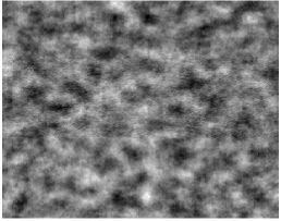
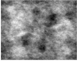
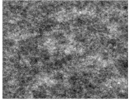
Figure 1: Illustrations of zero-mean Gaussian random fields. Left: Moving average spatial process. Middle: Stationary Gaussian random field on the torus. Right: Gaussian Markov random field.

2.1 Gaussian Property

A stochastic process $\{\widetilde{X}_{\mathbf{t}},\mathbf{t}\in\mathscr{T}\}$ is said to be Gaussian if all its finite-dimensional distributions are Gaussian (normal). That is, if for any choice of $n$ and $\mathbf{t}_{1},\ldots,\mathbf{t}_{n}\in\mathscr{T}$, we have

$$\mathbf{X}\stackrel{{\scriptstyle\text{def}}}{{=}}(X_{1},\ldots,X_{n})^{\top}\stackrel{{\scriptstyle\text{def}}}{{=}}(\widetilde{X}_{\mathbf{t}_{1}},\ldots,\widetilde{X}_{\mathbf{t}_{n}})^{\top}\sim{\sf N}(\boldsymbol{\mu},\Sigma)$$ (1)

for some expectation vector $\boldsymbol{\mu}$ and covariance matrix $\Sigma$. Hence, any linear combination $\sum_{i=1}^{n}b_{i}\widetilde{X}_{\mathbf{t}_{i}}$ has a normal distribution. A Gaussian process is determined completely by its expectation function $\widetilde{\mu}_{\mathbf{t}}=\mathbb{E}\widetilde{X}_{\mathbf{t}}$ and covariance function $\widetilde{\Sigma}_{\mathbf{s},\mathbf{t}}=\text{Cov}(\widetilde{X}_{\mathbf{s}},\widetilde{X}_{\mathbf{t}})$. To generate a Gaussian process with expectation function $\widetilde{\mu}_{\mathbf{t}}$ and covariance function $\widetilde{\Sigma}_{\mathbf{s},\mathbf{t}}$ at positions $\mathbf{t}_{1},\ldots,\mathbf{t}_{n}$, one can sample the multivariate normal random vector in (1) via the following algorithm.

Algorithm 2.1 (Gaussian Process Generator)

1. Construct the mean vector ${\boldsymbol{\mu}}=({\mu}_{1},\ldots,{\mu}_{n})^{\top}$ and covariance matrix ${\Sigma}=({\Sigma}_{ij})$ by setting ${\mu}_{i}=\widetilde{\mu}_{\mathbf{t}_{i}},i=1,\ldots,n$ and ${\Sigma}_{ij}=\widetilde{\Sigma}_{\mathbf{t}_{i},\mathbf{t}_{j}}$, $i,j=1,\ldots,n$.

2. Find a square root $A$ of $\Sigma$, so that $\Sigma=AA^{\top}$.

3. Generate $Z_{1},\ldots,Z_{n}\stackrel{{\scriptstyle\text{iid}}}{{\sim}}{{\sf N}}(0,1).$ Let $\mathbf{Z}=(Z_{1},\ldots,Z_{n})^{\top}$.

4. Output ${\mathbf{X}}=\boldsymbol{\mu}+A\mathbf{Z}$.

Using Cholesky’s square-root method, it is always possible to find a real-valued lower triangular matrix $A$ such that $\Sigma=AA^{\top}$. Sometimes it is easier to work with a decomposition of the form $\Sigma=BB^{*}$, where $B=B_{1}+\mathrm{i}B_{2}$ is a complex matrix with conjugate transpose $B^{*}=B_{1}^{\top}-\mathrm{i}B_{2}^{\top}$. Let $\mathbf{Z}=\mathbf{Z}_{1}+\mathrm{i}\mathbf{Z}_{2}$, where $\mathbf{Z}_{1}$ and $\mathbf{Z}_{2}$ are independent standard normal random vectors, as in Step 3 above. Then, the random vector $\mathbf{X}=\Re(B\mathbf{Z})=B_{1}\mathbf{Z}_{1}-B_{2}\mathbf{Z}_{2}$ has covariance matrix $\Sigma$.

A Gaussian vector $\mathbf{X}\sim{\sf N}(\boldsymbol{\mu},\Sigma)$ can also be simulated using its precision matrix $\Lambda=\Sigma^{-1}$. Let $\mathbf{Z}=D^{\top}\mathbf{Y}$, where $\mathbf{Z}\stackrel{{\scriptstyle\text{iid}}}{{\sim}}{{\sf N}}(0,1)$. If $DD^{\top}$ is the (lower) Cholesky factorization of $\Lambda$, then $\mathbf{Y}$ is a zero-mean multivariate normal vector with covariance matrix

$$\mathbb{E}\mathbf{Y}\mathbf{Y}^{\top}=(D^{-1})^{\top}\mathbb{E}\mathbf{Z}\mathbf{Z}^{\top}D^{-1}=(DD^{\top})^{-1}=\Lambda^{-1}=\Sigma\;.$$

The following algorithm describes how a Gaussian process can be generated using a precision matrix.

Algorithm 2.2 (Gaussian Process Generator Using a Precision Matrix)

1. Derive the Cholesky decomposition $\Lambda=DD^{\top}$ of the precision matrix.

2. Generate $Z_{1},\ldots,Z_{n}\stackrel{{\scriptstyle\text{iid}}}{{\sim}}{\sf N}(0,1)$. Let $\mathbf{Z}=(Z_{1},\ldots,Z_{n})^{\top}$.

3. Solve $\mathbf{Y}$ from $\mathbf{Z}=D^{\top}\mathbf{Y}$, using forward substitution.

4. Output $\mathbf{X}=\boldsymbol{\mu}+\mathbf{Y}$.

The Cholesky decomposition of a general $n\times n$ covariance or precision matrix takes $\mathcal{O}(n^{3})$ floating point operations. The generation of large-dimensional Gaussian vectors becomes very time-consuming for large $n$, unless some extra structure is introduced. In some cases the Cholesky decomposition can be altogether avoided by utilizing the fact that any Gaussian vector can be written as an affine transformation $\mathbf{X}=\boldsymbol{\mu}+A\mathbf{Z}$ of a “white noise” vector $\mathbf{Z}\stackrel{{\scriptstyle\text{iid}}}{{\sim}}{\sf N}(0,1)$; as in Step 4 of Algorithm 2.1. An example where such a transformation can be carried out directly is the following moving average Gaussian process $\mathbf{X}=\{X_{\mathbf{t}},\mathbf{t}\in\mathscr{T}\}$, where $\mathscr{T}$ is a two-dimensional grid of equally-spaced points. Here each $X_{\mathbf{t}}$ is equal to the average of all white noise terms $Z_{\mathbf{s}}$ with $\mathbf{s}$ lying in a disc of radius $r$ around $\mathbf{t}$. That is,

$$X_{\mathbf{t}}=\frac{1}{N_{r}}\sum_{\mathbf{s}\>:\>\|\mathbf{t}-\mathbf{s}\|\leqslant r}Z_{\mathbf{s}}\;,$$

where $N_{r}$ is the number of grid points in the disc. Such spatial processes have been used to describe rough energy surfaces for charge transport [5, 18]. The following $\mathrm{M}\mathrm{{\scriptstyle ATLAB}}$ program produces a realization of this process on a $200\times 200$ grid, using a radius $r=6$. A typical outcome is depicted in the left pane of Figure 1.

n = 300;
r = 6; % radius (maximal 49)
noise =  randn(n);
[x,y]=meshgrid(-r:r,-r:r);
mask=((x.^2+y.^2)<=r^2);  %(2*r+1)x(2*r+1) bit mask
x = zeros(n,n);
nmin = 50; nmax = 250;
for i=nmin:nmax
    for j=nmin:nmax
        A = noise((i-r):(i+r), (j-r):(j+r));
        x(i,j) = sum(sum(A.*mask));
    end
end
Nr = sum(sum(mask)); x = x(nmin:nmax, nmin:nmax)/Nr;
imagesc(x); colormap(gray)

2.2 Generating Stationary Processes via Circulant embedding

Another approach to efficiently generate Gaussian spatial processes is to exploit the structural properties of stationary Gaussian processes. A Gaussian process $\{\widetilde{X}_{\mathbf{t}},\mathbf{t}\in\mathbb{R}^{d}\}$ is said to be stationary if the expectation function, $\mathbb{E}\widetilde{X}_{\mathbf{t}}$, is constant and the covariance function, Cov$(\widetilde{X}_{\mathbf{s}},\widetilde{X}_{\mathbf{t}})$, is invariant under translations; that is $\text{Cov}(\widetilde{X}_{\mathbf{s}+\mathbf{u}},\widetilde{X}_{\mathbf{t}+\mathbf{u}})=\text{Cov}(\widetilde{X}_{\mathbf{s}},\widetilde{X}_{\mathbf{t}})\,.$

An illustrative example is the generation of a stationary Gaussian on the unit torus; that is, the unit square $[0,1]\times[0,1]$ in which points on opposite sides are identified with each other. In particular, we wish to generate a zero-mean Gaussian random process $\{\widetilde{X}_{\mathbf{t}}\}$ on each of the grid points $\{(i,j)/n,i=0,\ldots,n-1,j=0,\ldots,n-1\}$ corresponding to a covariance function of the form

$$\text{Cov}(\widetilde{X}_{\mathbf{s}},\widetilde{X}_{\mathbf{t}})=\exp\{-c\,\|\mathbf{s}-\mathbf{t}\|_{T}^{\alpha}\},$$ (2)

where $\|\mathbf{s}-\mathbf{t}\|_{T}=\|(s_{1}-t_{1},s_{2}-t_{2})\|_{T}\stackrel{{\scriptstyle\text{def}}}{{=}}\sqrt{\sum_{k=1}^{2}(\min\{|s_{k}-t_{k}|,1-|s_{k}-t_{k}|\})^{2}}$ is the Euclidean distance on the torus. Notice that this renders the process not only stationary but also isotropic (that is, the distribution remains the same under rotations). We can arrange the grid points in the order $(0,0),(0,1/n),\ldots,(0,1-1/n),(1/n,0),\ldots,(1-1/n,1-1/n)$. The values of the Gaussian process can be accordingly gathered in an $n^{2}\times 1$ vector $\mathbf{X}$ or, alternatively an $n\times n$ matrix $\underline{\mathbf{X}}$. Let $\Sigma$ be the $n^{2}\times n^{2}$ covariance matrix of $\mathbf{X}$. The key to efficient generation of $\mathbf{X}$ is that $\Sigma$ is a symmetric block-circulant matrix with circulant blocks. That is, $\Sigma$ has the form

$$\Sigma=\begin{pmatrix}C_{1}&C_{2}&C_{3}&\ldots&C_{n}\\ C_{n}&C_{1}&C_{2}&\ldots&C_{n-1}\\ &&\ldots&&\\ C_{2}&C_{3}&\ldots&C_{n}&C_{1}\end{pmatrix},$$

where each $C_{i}$ is a circulant matrix $\text{circ}(c_{i1},\ldots,c_{in})$. The matrix $\Sigma$ is thus completely specified by its first row, which we gather in an $n\times n$ matrix $G$. The eigenstructure of block-circulant matrices with circulant blocks is well known; see, for example, [4]. Specifically, $\Sigma$ is of the form

$$\Sigma=P^{*}\text{diag}(\boldsymbol{\gamma})P,$$ (3)

where $P^{*}$ denotes the complex conjugate transpose of $P$, and $P$ is the Kronecker product of two discrete Fourier transform matrices; that is, $P=F\otimes F$, where $F_{jk}=\exp(-2\pi\mathrm{i}jk/n)/\sqrt{n},j,k=0,1,\ldots,n-1.$ The vector of eigenvalues $\boldsymbol{\gamma}=(\gamma_{1},\ldots,\gamma_{n^{2}})^{\top}$ ordered as an $n\times n$ matrix $\Gamma$ satisfies $\Gamma=n\,F^{*}GF$. Since $\Sigma$ is a covariance matrix, the component-wise square root $\sqrt{\Gamma}$ is well-defined and real-valued. The matrix $B=P^{*}\text{diag}(\sqrt{\boldsymbol{\gamma}})$ is a complex square root of $\Sigma$, so that $\mathbf{X}$ can be generated by drawing $\mathbf{Z}=\mathbf{Z}_{1}+\mathrm{i}\mathbf{Z}_{2}$, where $\mathbf{Z}_{1}$ and $\mathbf{Z}_{2}$ are independent standard normal random vectors, and returning the real part of $B\mathbf{Z}$. It will be convenient to gather $\mathbf{Z}$ into an $n\times n$ matrix $\underline{\mathbf{Z}}$.

The evaluation of both $\Gamma$ and $\underline{\mathbf{X}}$ can be done efficiently by using the (appropriately scaled) two-dimensional Fast Fourier Transform (FFT2). In particular, $\Gamma$ is the FFT2 of the matrix $G$ and $\underline{\mathbf{X}}$ is the real part of the FFT2 of the matrix $\sqrt{\Gamma}\odot\underline{\mathbf{Z}}$, where $\odot$ denotes component-wise multiplication. The following $\mathrm{M}\mathrm{{\scriptstyle ATLAB}}$ program generates the outcome of a stationary Gaussian random field on a $256\times 256$ grid, for a covariance function of the form (2), with $c=8$ and $\alpha=1$. The realization is shown in the middle pane of Figure 1.

n = 2^8;
t1 = [0:1/n:1-1/n]; t2 = t1;
for i=1:n   % first row of cov. matrix, arranged in a matrix
  for j=1:n
       G(i,j)=exp(-8*sqrt(min(abs(t1(1)-t1(i)), ...
       1-abs(t1(1)-t1(i)))^2 + min(abs(t2(1)-t2(j)), ...
       1-abs(t2(1)-t2(j)))^2));
  end;
end;
Gamma = fft2(G);   % the eigenvalue matrix n*fft2(G/n)
Z = randn(n,n) + sqrt(-1)*randn(n,n);
X = real(fft2(sqrt(Gamma).*Z/n));
imagesc(X); colormap(gray)

Dietrich and Newsam [10] and Wood and Chan [7, 34] discuss the generation of general stationary Gaussian processes in $\mathbb{R}^{d}$ with covariance function

$$\text{Cov}(\widetilde{X}_{\mathbf{s}},\widetilde{X}_{\mathbf{t}})=\varrho(\mathbf{s}-\mathbf{t})\;.$$

Recall that if $\varrho(\mathbf{s}-\mathbf{t})=\varrho(\|\mathbf{s}-\mathbf{t}\|)$, then the random field is not only stationary, but isotropic.

Dietrich and Newsam propose the method of circulant embedding, which allows the efficient generation of a stationary Gaussian field via the FFT. The idea is to embed the covariance matrix into a block circulant matrix with each block being circulant itself (as in the last example), and then construct the matrix square root of the block circulant matrix using FFT techniques. The FFT permits the fast generation of the Gaussian field with this block circulant covariance matrix. Finally, the marginal distribution of appropriate sub-blocks of this Gaussian field have the desired covariance structure.

Here we consider the two-dimensional case. The aim is to generate a zero-mean stationary Gaussian field over the $n\times m$ rectangular grid

$${{\cal G}}=\{(i\Delta_{x},j\Delta_{y}),\;i=0,\ldots,n-1,\;j=0,\ldots,m-1\},$$

where $\Delta_{x}$ and $\Delta_{y}$ denote the corresponding horizontal and vertical spacing along the grid. The algorithm can broadly be described as follows.

Step 1. Building and storing the covariance matrix. The grid points can be arranged into a column vector of size $n\,m$ to yield the $m^{2}n^{2}$ covariance matrix $\Omega_{i,j}=\varrho(\mathbf{s}_{i}-\mathbf{s}_{j}),\;i,j=1,\ldots,m\,n$, where

$$\mathbf{s}_{k}\stackrel{{\scriptstyle\text{def}}}{{=}}\left((k-1)\mod m,\quad\left\lfloor\frac{k}{m}\right\rfloor\right),\quad k=1,\ldots,m\,n\;.$$

The matrix $\Omega$ has symmetric block-Toeplitz structure, where each block is a Toeplitz (not necessarily symmetric) matrix. For example, the left panel of Figure 2 shows the block-Toeplitz covariance matrix with $m=n=3$. Each $3\times 3$ block is itself a Toeplitz matrix with entry values coded in color. For instance, we have $\Omega_{2,4}=\Omega_{3,5}=c$.

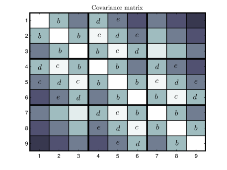
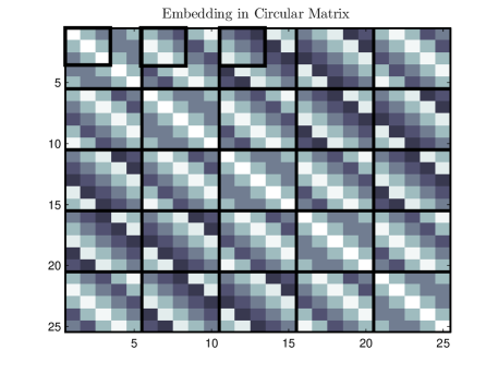
Figure 2: Left panel: the symmetric block-Toeplitz covariance matrix $\Omega$ with $n=m=3$. Right panel: block-circulant matrix $\Sigma$ of size $((2n-1)\times(2m-1))^{2}=25\times 25$. The first three block rows of $\Omega$ are embedded in the upper left corners of the first three block columns of the circulant matrix $\Sigma$.

Matrix $\Omega$ is thus uniquely characterized by its first block row $(R_{1},\ldots,R_{n})$ where each of the $n$ blocks is an $m\times m$ Toeplitz matrix. The $k$-th $m\times m$ Toeplitz matrix consists of the sub-block of $\Omega$ with entries

$$\Omega_{i,j},\quad i=1,\ldots,m,\;j=(km+1),\ldots,(k+1)m\;.$$

Notice that each block $R_{k}$ is itself characterized by its first row and column. (Each Toeplitz block $R_{k}$ will be characterized by the first row only provided the covariance function has the form $\varrho(\mathbf{s}-\mathbf{t})=\varrho(\|\mathbf{s}\|,\|\mathbf{t}\|)$, in which case each $R_{k}$ is symmetric.) Thus, in general the covariance matrix can be completely characterized by the entries of a pair of $m\times n$ and $n\times m$ matrices storing the first columns and rows of all $n$ Toeplitz blocks $(R_{1},\ldots,R_{n})$. In typical applications, the computation of these two matrices is the most time-consuming step.

Step 2. Embedding in block circulant matrix. Each Toeplitz matrix $R_{k}$ is embedded in the upper left corner of an $2m+1$ circulant matrix $C_{k}$. For example, in the right panel of Figure 2 the embedded blocks $R_{1},R_{2},R_{3}$ are shown within bold rectangles. Finally, let $\Sigma$ be the $(2n-1)(2m-1)\times(2n-1)(2m-1)$ block circulant matrix with first block row given by $(C_{1},\ldots,C_{n},C_{n}^{\top},\ldots,C_{2}^{\top}).$ This gives the minimal embedding in the sense that there is no block circulant matrix of smaller size that embeds $\Omega$.

Step 3. Computing the square root of the block circulant matrix. After the embedding we are essentially generating a Gaussian process on a torus with covariance matrix $\Sigma$ as in the last example. The block circulant matrix $\Sigma$ can be diagonalized as in (3) to yield $\Sigma=P^{*}\text{diag}(\boldsymbol{\gamma})P$, where $P$ is the $(2n-1)(2m-1)\times(2n-1)(2m-1)$ two-dimensional discrete Fourier transform matrix. The vector of eigenvalues $\boldsymbol{\gamma}$ is of length $(2n-1)(2m-1)$ and is arranged in a $(2m-1)\times(2n-1)$ matrix $\Gamma$ so that the first column of $\Gamma$ consists of the first $2m-1$ entries of $\boldsymbol{\gamma}$, the second column of $\Gamma$ consists of the next $2m-1$ entries and so on. It follows that if $G$ is an $(2m-1)\times(2n-1)$ matrix storing the entries of the first block row of $\Sigma$, then $\Gamma$ is the FFT2 of $G$. Assuming that $\boldsymbol{\gamma}>0$, we obtain the square root factor $B=P^{*}\text{diag}(\sqrt{\boldsymbol{\gamma}})$, so that $\Sigma=B^{*}B$.

Step 4. Extracting the appropriate sub-block. Next, we compute the FFT2 of the array $\sqrt{\Gamma}\odot\underline{\mathbf{Z}}$, where the square root is applied component-wise to $\Gamma$ and $\underline{\mathbf{Z}}$ is an $(2m-1)\times(2n-1)$ complex Gaussian matrix with entries $\underline{\mathbf{Z}}_{j,k}=U_{j,k}+\mathrm{i}V_{j,k}$, $U_{j,k},V_{j,k}\stackrel{{\scriptstyle\text{iid}}}{{\sim}}{\sf N}(0,1)$ for all $j$ and $k$. Finally, the first $m\times n$ sub-blocks of the real and imaginary parts of $\mathrm{FFT2}(\sqrt{\Gamma}\odot\underline{\mathbf{Z}})$ represent two independent realization of a stationary Gaussian field with covariance $\Sigma$ on the grid ${{\cal G}}$. If more realizations are required, we store the values $\sqrt{\Gamma}$ and we repeat Step 4 only. The complexity of the circulant embedding inherits the complexity of the FFT approach, which is of order $\mathcal{O}(mn\ln(m+n))$, and compares very favorably with the standard Cholesky decomposition method of order $\mathcal{O}(m^{3}n^{3})$.

As a numerical example (see [10]), Figure 3 shows a realization of a stationary nonisotropic Gaussian field with $m=512,n=384,\;\Delta_{x}=\Delta_{y}=1$, and covariance function

$$\varrho(\mathbf{s}-\mathbf{t})=\varrho(\mathbf{h})=\left(1-\frac{h_{1}^{2}}{50^{2}}-\frac{h_{1}h_{2}}{50\times 15}-\frac{h_{2}^{2}}{15^{2}}\right)\exp\left(-\frac{h_{1}^{2}}{50^{2}}-\frac{h_{2}^{2}}{15^{2}}\right)\;.$$ (4)

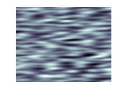
Figure 3: Realization of a stationary nonisotropic Gaussian field with covariance function (4).

The following $\mathrm{M}\mathrm{{\scriptstyle ATLAB}}$ code implements the procedure described above with covariance function (4).

n=384; m=512; % size of grid is m*n
% size of covariance matrix is m^2*n^2
tx=[0:n-1]; ty=[0:m-1]; % create grid for field
rho=@(x,y)((1-x^2/50^2-x*y/(15*50)-y^2/15^2)...
      *exp(-(x^2/50^2+y^2/15^2)));
Rows=zeros(m,n); Cols=Rows;
for i=1:n
    for j=1:m
        Rows(j,i)=rho(tx(i)-tx(1),ty(j)-ty(1)); % rows of blocks
        Cols(j,i)=rho(tx(1)-tx(i),ty(j)-ty(1)); % columns
    end
end
% create the first row of the block circulant matrix
% with circulant blocks and store it as a matrix suitable for fft2
BlkCirc_row=[Rows, Cols(:,end:-1:2);
    Cols(end:-1:2,:), Rows(end:-1:2,end:-1:2)];
% compute eigen-values
lam=real(fft2(BlkCirc_row))/(2*m-1)/(2*n-1);

if abs(min(lam(lam(:)<0)))>10^-15
    error(’Could not find positive definite embedding!’)
else
    lam(lam(:)<0)=0; lam=sqrt(lam);
end
% generate field with covariance given by block circulant matrix
F=fft2(lam.*complex(randn(2*m-1,2*n-1),randn(2*m-1,2*n-1)));
F=F(1:m,1:n); % extract sub-block with desired covariance
field1=real(F); field2=imag(F); % two independent fields
imagesc(tx,ty,field1), colormap bone

Extensions to three and more dimensions are possible, see [10]. For example, in the three dimensional case the correlation matrix $\Omega$ will be symmetric block Toeplitz matrix with each block satisfying the properties of a two dimensional covariance matrix.

Throughout the discussion so far we have always assumed that the block circulant matrix $\Sigma$ is a covariance matrix itself. If this is the case, then we say that we have a nonnegative definite embedding of $\Omega$. A nonnegative definite embedding ensures that the square root of $\boldsymbol{\gamma}$ is real. Generally, if the correlation between points on the grid that are sufficiently far apart is zero, then a non-negative embedding will exist, see [10]. A method that exploits this observation is the intrinsic embedding method proposed by Stein [30] (see also [13]). Stein’s method depends on the construction of a compactly supported covariance function that yields to a nonnegative circulant embedding. The idea is to modify the original covariance function so that it decays smoothly to zero. In more detail, suppose we wish to simulate a process with covariance $\varrho$ over the set $\{\mathbf{h}:\|\mathbf{h}\|\leqslant 1,\mathbf{h}>\mathbf{0}\}$. To achieve this, we simulate a process with covariance function

$$\psi(\mathbf{h})=\begin{cases}c_{0}+c_{2}\|\mathbf{h}\|^{2}+\varrho(\mathbf{h}),&\|\mathbf{h}\|\leqslant 1\\ \phi(\mathbf{h}),&1\leqslant\|\mathbf{h}\|\leqslant R\\ 0,&\|\mathbf{h}\|\geqslant R\end{cases},$$ (5)

where the constants $c_{0},c_{2},\;R\geqslant 1$ and function $\phi$ are selected so that $\psi$ is a continuous (and as many times differentiable as possible), stationary and isotropic covariance function on $\mathbb{R}^{2}$. The process will have covariance structure of $c_{0}+c_{2}\|\mathbf{h}\|^{2}+\varrho(\mathbf{h})$ in the disk $\{\mathbf{h}:\|\mathbf{h}\|\leqslant 1,\mathbf{h}>\mathbf{0}\}$, which can then be easily transformed into a process with covariance $\varrho(\mathbf{h})$. We give an example of this in Section 4.4, where we generate fractional Brownian surfaces via the intrinsic embedding technique. Generally, the smoother the original covariance function, the harder it is to embed via Stein’s method, because a covariance function that is smoother close to the origin has to be even smoother elsewhere.

2.3 Markov Property

A Markov random field is a spatial stochastic process $\mathbf{X}=\{X_{\mathbf{t}},\mathbf{t}\in\mathscr{T}\}$ that possesses a Markov property, in the sense that

$$(X_{\mathbf{t}}\,|\,X_{\mathbf{s}},\mathbf{s}\in\mathscr{T}\setminus\{\mathbf{t}\})\sim(X_{\mathbf{t}}\,|\,X_{\mathbf{s}},\mathbf{s}\in\mathscr{N}_{\mathbf{t}}),$$

where $\mathscr{N}_{\mathbf{t}}$ is the set of “neighbors” of $\mathbf{t}$. Thus, for each $\mathbf{t}\in\mathscr{T}$ the conditional distribution of $X_{\mathbf{t}}$ given all other values $X_{\mathbf{s}}$ is equal to the conditional distribution of $X_{\mathbf{t}}$ given only the neighboring values.

Markov random fields are often defined via an undirected graph ${\cal G}=({V},{E})$. In such a graphical model the vertices of the graph correspond to the indices $\mathbf{t}\in\mathscr{T}$ of the random field, and the edges describe the dependencies between the random variables. In particular, there is no edge between nodes $\mathbf{s}$ and $\mathbf{t}$ in the graph if and only if $X_{\mathbf{s}}$ and $X_{\mathbf{t}}$ are conditionally independent, given all other values $\{X_{\mathbf{u}},\mathbf{u}\neq i,j\}$. In a Markov random field described by a graph $\cal G$, the set of neighbors $\mathscr{N}_{\mathbf{t}}$ of $\mathbf{t}$ corresponds to the set of vertices that share an edge with $\mathbf{t}$; that is, those vertices that are adjacent to $\mathbf{t}$. An example of a graphical model for a 2-dimensional Markov random field is shown in Figure 4. In this case vertex corner nodes have two neighbors and interior nodes have four neighbors.

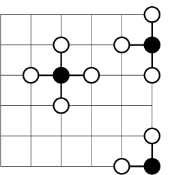
Figure 4: A graphical model for 2D spatial process. Each vertex has at most four neighbors.

Of particular importance are Markov random fields that are also Gaussian. Suppose $\mathbf{X}$ is such a Gaussian Markov random field (GMRF), with corresponding graphical model ${\cal G}=(V,E)$. We may think of $\mathbf{X}$ as a column vector of $n=|V|$ elements, or as a spatial arrangement of random variables (pixel values), as in Figure 4. Without loss of generality we assume that $\mathbb{E}\mathbf{X}=\boldsymbol{0}$, and that the index set $\mathscr{T}$ is identified with the vertex set $V$, whose elements are labeled as $1,2,\ldots,n$. Because $\mathbf{X}$ is Gaussian, its pdf is given by

$$f(\mathbf{x})=(2\pi)^{-n/2}\sqrt{\det(\Lambda)}\>\text{e}^{-\frac{1}{2}\mathbf{x}^{\top}\Lambda\mathbf{x}}\;,$$

where $\Lambda=(\lambda_{ij})$ is the precision matrix. In particular, the conditional joint pdf of $X_{i}$ and $X_{j}$ is

$$f(x_{i},x_{j}\,|\,x_{k},k\neq i,j)\propto\exp\left(-\frac{1}{2}(\lambda_{ii}x_{i}^{2}+2x_{i}\,a+\lambda_{ij}x_{i}x_{j}+\lambda_{jj}x_{j}^{2}+2x_{j}\,b)\right),$$

where $a$ and $b$ may depend on $x_{k},k\neq i,j$. This shows that $X_{i}$ and $X_{j}$ are conditionally independent given $\{X_{k},k\neq i,j\}$, if and only if $\lambda_{ij}=0$. Consequently, $(i,j)$ is an edge in the graphical model if and only if $\lambda_{ij}\neq 0$. In typical applications (for example in image analysis) each vertex in the graphical model only has a small number of adjacent vertices, as in Figure 4. In such cases the precision matrix is thus sparse, and the Gaussian vector can be generated efficiently using, for example, sparse Cholesky factorization [14].

As an illustrative example, consider the graphical model of Figure 4 on a grid of $n=m^{2}$ points: $\{1,\ldots,m\}\times\{1,\ldots,m\}$. We can efficiently generate a GMRF on this grid via Algorithm 2.2, provided the Cholesky decomposition can be carried out efficiently. For this we can use for example the band Cholesky method [14], which takes $n(p^{2}+3p)$ floating point operations, where $p$ is the bandwidth of the matrix; that is, $p=\max_{i,j}\{|i-j|:\lambda_{ij}=0\}$. The right pane of Figure 1 shows a realization of the GMRF on a $250\times 250$ grid, using parameters $\lambda_{ii}=2$ for all $i=1,\ldots,n$ and $\lambda_{ij}=-0.5$ for all neighboring elements $j\in{\cal N}_{j}$ of $i=1,\ldots,n$. The $\mathrm{M}\mathrm{{\scriptstyle ATLAB}}$ code may be found in Section 5.1 of [19]. Further details on such construction methods for GMRFs may be found, for example, in the monograph by Rue and Held [28].

3 Point Processes

Point processes on $\mathbb{R}^{d}$ are spatial processes describing random configurations of $d$-dimensional points. Spatially distributed point patterns occur frequently in nature and in a wide variety of scientific disciplines such as spatial epidemiology, material science, forestry, geography. The positions of accidents on a highway during a fixed time period, and the times of earthquakes in Japan are examples of one-dimensional spatial point processes. Two-dimensional examples include the positions of cities on a map, the positions of farms with Mad Cow Disease in the UK, and the positions of broken connections in a communications or energy network. In three dimensions, we observe the positions of stars in the universe, the positions of mineral deposits underground, or the times and positions of earthquakes in Japan. Spatial processes provide excellent models for many of these point patterns [2, 3, 9, 11]. Spatial processes also have an important role in stochastic modeling of complex microstructures, for example, graphite electrodes used in Lithium-ion batteries [31].

Mathematically, point processes can be described in three ways: (1) as random sets of points, (2) as random-sized vectors of random positions, and (3) as random counting measures. In this section we discuss some of the important point processes and their generalizations, including Poisson processes, marked point processes, and cluster processes.

3.1 Poisson Process

Poisson processes are used to model random configurations of points in space and time. Let $E$ be some subset of $\mathbb{R}^{d}$ and let ${\cal E}$ be the collection of (Borel) sets on $E$. To any collection of random points $\{X_{1},\ldots,X_{N}\}$ in $E$ corresponds a random counting measure $\mathbf{X}(A),A\in{\cal E}$ defined by

$$\mathbf{X}(A)=\sum_{i=1}^{N}\text{I}_{\{X_{i}\in A\}},\quad A\in{\cal E}\;,$$ (6)

which counts the random number of points in $A$. We may identify the random measure $\mathbf{X}$ defined in (6) with the random set $\{X_{i},i=1,\ldots,N\}$, or with the random vector $(X_{1},\ldots,X_{N})$. Note that the $d$-dimensional points $x_{i},X_{i}$ etc. are not written in boldface font here, in contrast to Section 2. The measure $\mu(A)=\mathbb{E}\mathbf{X}(A),A\in{\cal E}$ is called the mean measure of $\mathbf{X}$. In most practical cases the mean measure $\mu$ has a density $\lambda$, called the intensity; so that

$$\mu(A)=\mathbb{E}\mathbf{X}(A)=\int_{A}\lambda(x)\,\text{d}x\;.$$

We will assume from now on that such an intensity function exists.

The most important point process which holds the key to the analysis of point pattern data is the Poisson process. A random counting measure $\mathbf{X}$ is said to be a Poisson random measure with mean measure $\mu$ if the following properties hold:

1. For any set $A\in{\cal E}$ the random variable $\mathbf{X}(A)$ has a Poisson distribution with mean $\mu(A)$. We write $\mathbf{X}(A)\sim{\sf Poi}(\mu(A))$.

2. For any disjoint sets $A_{1},\dots,A_{N}\in{\cal E}$, the random variables $\mathbf{X}(A_{1}),\dots,\mathbf{X}(A_{N})$ are independent.

The Poisson process is said to be homogeneous if the intensity function is constant. An important corollary of Properties 1 and 2 is:

1. Conditional upon $\mathbf{X}(E)=N$, the points $X_{1},\ldots,X_{N}$ are independent of each other and have pdf $g(x)=\lambda(x)/\mu(E)$.

This result is the key to generating a Poisson random measure on $\mathbb{R}^{d}$.

Algorithm 3.1 (Generating a Poisson Random Measure)

• Generate a Poisson random variable $N\sim{{\sf Poi}}(\mu(E))$.

• Draw $X_{1},\ldots,X_{N}\stackrel{{\scriptstyle\text{iid}}}{{\sim}}g$, where $g(x)=\lambda(x)/\mu(E)$, and return these as the points of the Poisson random measure.

As a specific example, consider the generation of a 2-dimensional Poisson process with intensity $\lambda(x_{1},x_{2})=300(x_{1}^{2}+x_{2}^{2})$ on the unit square $E=[0,1]^{2}$. Since the pdf $g(x_{1},x_{2})=\lambda(\mathbf{x})/\mu(E)=3(x_{1}^{2}+x_{2}^{2})/2$ is bounded by 3, drawing from $g$ can be done simply via the acceptance–rejection method [27]. That is, draw $(X_{1},X_{2})$ uniformly on $E$ and $Z$ uniformly on $[0,3]$, and accept $(X_{1},X_{2})$ if $g(X_{1},X_{2})\leqslant Z$; otherwise repeat. This acceptance–rejection step is then repeated $N\sim{\sf Poi}(200)$ times. An alternative, but equivalent, method is to generate a homogeneous Poisson process on $E$, with intensity $\lambda^{*}=600$, and to thin out the points by accepting each point $\mathbf{x}$ with probability $\lambda(x_{1},x_{2})/\lambda^{*}$. The following $\mathrm{M}\mathrm{{\scriptstyle ATLAB}}$ implements this thinning procedure. A typical realization is given in Figure 5.

lambda = @(x) 300*(x(:,1).^2 + x(:,2).^2);
lamstar = 600;
N=poissrnd(lamstar); x = rand(N,2); % homogeneous PP
ind = find(rand(N,1) < lambda(x)/lamstar);
xa = x(ind,:); % thinned PP
plot(xa(:,1),xa(:,2))

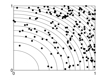
Figure 5: A realization of a nonhomogeneous Poisson process with intensity $\lambda(x_{1},x_{2})=300(x_{1}^{2}+x_{2}^{2})$ (contour lines shown) on the unit square.

3.2 Marked Point Processes

A natural way to extend the notion of a point process is to associate with each point $X_{i}\in\mathbb{R}^{d}$ a mark $Y_{i}\in\mathbb{R}^{m}$, representing an attribute such as width, velocity, weight etc. The collection $\{(X_{i},Y_{i})\}$ is called a marked point process. In a marked point process with independent marking the marks are assumed to be independent of each other and of the points, and distributed according to a fixed mark distribution. The following gives a useful connection between marked point processes and Poisson processes; see, for example, [9].

Theorem 3.1

If $\{(X_{i},Y_{i})\}$ is a Poisson process on $\mathbb{R}^{d}\times\mathbb{R}^{m}$ with intensity $\zeta$, and $K(x)=\int\zeta(x,y)\,\text{d}y<\infty$ for all $x$, then $\{X_{i}\}$ is a Poisson process on $\mathbb{R}^{d}$ with intensity $K$, and $\{(X_{i},Y_{i})\}$ is a marked Poisson process with mark density $\zeta(x,\cdot)/K(x)$ on $\mathbb{R}^{m}$.

A (spatial) marked Poisson process with independent marking is an important example of a (spatial) Lévy process: a stochastic process with independent and stationary increments (discussed in more detail in Section 5).

The generation of a marked Poisson process with independent marks is virtually identical to that of an ordinary (that is, non-marked) Poisson process. The only difference is that for each point the mark has to be drawn from the mark distribution. An example of a realization of a marked Poisson process is given in Figure 6. Here the marks are uniformly distributed on [0,0.1], and the underlying Poisson process is homogeneous with intensity 100.

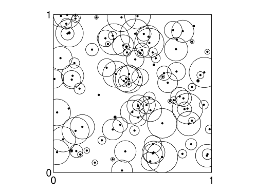
Figure 6: A realization of a marked Poisson process with independent marking on the unit square. The Poisson process has intensity 100. The marks are uniformly distributed on [0,0.1] and correspond to the radii of the circles.

3.3 Cluster Process

In nature one often observes point patterns that display clustering. An example is the spread of plants from a weed species where the plants are initially introduced by birds at a number of geographically dispersed locations and the plants then spread themselves locally.

Let ${\bf C}$ be a point process of “centers” and associate with each $c\in{\bf C}$ a point process $\mathbf{X}^{c}$, which may include $c$. The combined set of points $\mathbf{X}=\cup_{c\in{\bf C}}\mathbf{X}^{c}$ constitutes a cluster process. If ${\bf C}$ is a Poisson process, then $\mathbf{X}$ is called a Poisson cluster process.

As a specific example, consider the following Hawkes process. Here, the center process ${\bf C}$ is a Poisson process on $\mathbb{R}^{d}$ (or a subset thereof) with some intensity function $\lambda(\cdot)$. The clusters are generated as follows. For each $c\in{\bf C}$, independently generate “first-generation offspring” according to a Poisson process with intensity $\varrho(x-c)$, where $\varrho(\cdot)$ is a positive function on $\mathbb{R}^{d}$ with integral less than unity. Then, for each first-generation offspring $c_{1}$ generate a Poisson process with intensity $\varrho(x-c_{1})$, and so on. The collection of all generated points forms the Hawkes process. The requirement that $\int\varrho(y)\,\text{d}y<1$ simply means that the expected number of offspring of each point is less than one.

Figure 7 displays a realization for $\mathbb{R}^{2}$ with the cluster centers forming a Poisson process on the unit square with intensity $\lambda=30$. The offspring intensity is here

$$\varrho(x_{1},x_{2})=\frac{\alpha}{2\pi\sigma^{2}}\text{e}^{-\frac{1}{2\sigma^{2}}(x_{1}^{2}+x_{2}^{2})},\quad(x_{1},x_{2})\in\mathbb{R}^{2},$$ (7)

with $\alpha=0.9$ and with $\sigma=0.02$. This means that the number $N$ of offspring for a single generation from a parent at position $(x_{1},x_{2})$ has a Poisson distribution with parameter $\alpha$. And given $N=n$, the offspring are iid distributed according to a bivariate normal random vector with independent components with means $x_{1}$ and $x_{2}$ and both variances $\sigma^{2}$. In Figure 7 the cluster centers are indicated by circles. Note that the process possibly has points outside the displayed box. The $\mathrm{M}\mathrm{{\scriptstyle ATLAB}}$ code is given below.

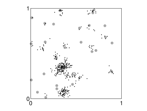
Figure 7: Realization of a two-dimensional Hawkes process with centers (encircled) forming a Poisson process on $[0,1]\times[0,1]$ with intensity $\lambda=30$. The offspring intensity is given in (7).

lambda = 30;           %intensity of initial points (centers)
mean_children = 0.9;   %mean number of children of each point
X = zeros(10^5,2);     %initialise the points
N = poissrnd(lambda);  %number of centers
X(1:N,:) = rand(N,2);  %generate the centers
total_so_far = N;      %total number of points generated
next = 1;
while next < total_so_far
    nextX = X(next,:);   %select next point
    N_children = poissrnd(mean_children);    %number of children
    NewX = repmat(nextX,N_children,1) + 0.02*randn(N_children,2);
    X(total_so_far+(1:N_children),:) = NewX;  %update point list
    total_so_far = total_so_far+N_children;
    next = next+1;
end
X=X(1:total_so_far,:); %cut off unused rows
plot(X(:,1),X(:,2),’.’)

3.4 Cox Process

Suppose we wish to model a point pattern of trees given that we know the soil quality $h(x_{1},x_{2})$ at each point $(x_{1},x_{2})$. We could use a non-homogeneous Poisson process with an intensity $\lambda$ that is an increasing function of $h$; for example, $\lambda(x_{1},x_{2})=\text{e}^{\alpha+\beta h(x_{1},x_{2})}$ for some known $\alpha>0$ and $\beta>0$. In practice, however, the soil quality itself could be random, and be described via a random field. Consequently, one could could try instead to model the point pattern as a Poisson process with a random intensity function $\Lambda$. Such processes were introduced by Cox as doubly stochastic Poisson processes and are now called Cox processes [8].

More precisely, we say that $\mathbf{X}$ is a Cox process driven by the random intensity function $\Lambda$ if conditional on $\Lambda$ the point process $\mathbf{X}$ is Poisson with intensity function $\lambda$. Simulation of a Cox process on a set $\mathscr{T}\subset\mathbb{R}^{d}$ is thus a two-step procedure.

Algorithm 3.2 (Simulation of a Cox Process)

1. Simulate a realization $\lambda=\{\lambda(x),x\in\mathscr{T}\}$ of the random intensity $\Lambda$.

2. Given $\Lambda=\lambda$, simulate $\mathbf{X}$ as an inhomogeneous Poisson process with intensity $\lambda$.

Figure 8 shows a realization of a Cox process on the unit square $\mathscr{T}=[0,1]\times[0,1]$, with a random intensity whose realization is given in Figure 8. The random intensity at position $(x_{1},x_{2})$ is either 3000 or 0, depending on whether the value of a random field on $\mathscr{T}$ is negative or not. The random field that we used is the stationary Gaussian process on the torus described in Section 2.

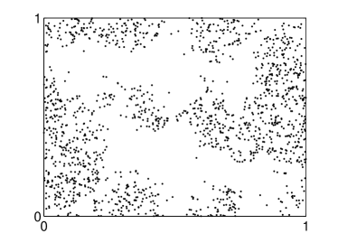
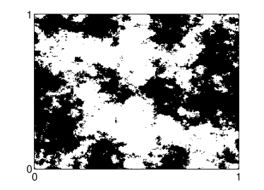
Figure 8: Realization of a Cox process: (a) on a square generated by a the random intensity function given in (b). The black points have intensity 3000 and the white points have intensity 0.

Given an outcome of the random intensity, the Cox process is constructed by generating a homogeneous Poisson process with rate $3000$ on $\mathscr{T}$ and accepting only those points for which the random intensity is non-zero. The value of the intensity is taken to be constant within each square $\{(i+u)/n,(j+v)/n),0\leqslant u,v\leqslant 1\}$, $i,j=0,\ldots,n-1$. The following $\mathrm{M}\mathrm{{\scriptstyle ATLAB}}$ code is to be appended to the code used for the stationary Gaussian process generation on the torus in Section 2.

Lambda = ones(n,n).*(X < 0); %random intensity
%imagesc(Lambda); set(gca,’YDir’,’normal’)
Lambda = Lambda(:); %reshape as a column vector
N = poissrnd(3000);
P = rand(N,2); %generate homogenous PP
Pn = ceil(P*n); %PP scaled by factor n
K = (Pn(:,1)-1)*n + Pn(:,2); % indices of scaled PP
ind = find(Lambda(K)); %indices for which intensity is 1
Cox = P(ind,:);  %realization of the Cox process
plot(Cox(:,1),Cox(:,2),’.’);

Neyman and Scott [25] applied the following Cox process to cosmology. Used to model the positions of stars in the universe, it now bears the name Neyman–Scott process. Suppose $\mathbf{C}$ is a homogeneous Poisson process in $\mathbb{R}^{d}$ with constant intensity $\kappa$. Let the random intensity $\Lambda$ be given by

$$\Lambda(x)=\alpha\sum_{c\in\mathbf{C}}k(x-c)$$

for some $\alpha>0$ and some $d$-dimensional probability density function $k$. Such a Cox process is also a Poisson cluster process. Note that in this case the cluster centers are not part of the Cox process. Given a realization of the cluster center process $\mathbf{C}$, the cluster of points originating from $c\in\mathbf{C}$ form a non-homogeneous Poisson process with intensity $k(x-c),x\in\mathbb{R}^{d}$, independently of the other clusters. Drawing such a cluster via Algorithm 3.1 simply means that (1) the number of points $N_{c}$ in the cluster has a ${\sf Poi}(\alpha)$ distribution, and (2) these $N_{c}$ points are iid distributed according to pdf $k(x-c)$.

A common choice for pdf $k$ is $k(x)\propto\text{I}_{\{\|x\|\leqslant r\}}$, first proposed by Matérn [23]. The resulting process is called a Matérn process. Thus, for a Matérn process each point in the cluster with center $c$ is uniformly distributed within a ball of radius $r$ at $c$. If instead a ${\sf N}(c,\sigma^{2}I)$ distribution is used, where $I$ is the $d$-dimensional identity matrix, then the process is known as a (modified) Thomas process [24].

Figure 9 shows a realization of a Matérn process with parameters $\kappa=20$, $\alpha=5$ and $r=0.1$ on $[0,1]\times[0,1]$. Note that the cluster centers are assumed to lie on the whole of $\mathbb{R}^{2}$. To show a genuine outcome of the process within the window $[0,1]\times[0,1]$ it suffices to consider only the points that are generated from centers lying in square $[-r,1+r]\times[-r,1+r]$.

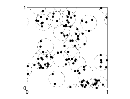
Figure 9: A realization of a Matérn process with parameters $\kappa=20$, $\alpha=5$, and $r=0.1$. The process extends beyond the shown window. The cluster centers (the centers of the circles) are not part of the point pattern.

The following $\mathrm{M}\mathrm{{\scriptstyle ATLAB}}$ program was used.

X = zeros(10^5,2);  %initialise the points
kappa = 20; alpha = 5; r = 0.1; %parameters
meanpts=kappa*(1 + 2*r)^2;
N = poissrnd(meanpts);     %number of cluster centers
C = rand(N,2)*(1+2*r) - r;  ;%draw cluster centers
total_so_far = 0;
for c=1:N
    NC = poissrnd(alpha);  %number of points in cluster
    k = 0;
    while k < NC %draw uniformly in the n-ball via accept-reject
        Y = 2*r*rand(1,2) - r; %candidate point
        if norm(Y) < r
            X(total_so_far+k+1,:) = C(c,:) + Y;
            k = k+1;
        end
    end
    total_so_far = total_so_far + NC;
end
X = X(1:total_so_far,:);    %cut off unused rows
plot(X(:,1),X(:,2),’.’)
axis([0, 1,0, 1])

A versatile generalization the Neyman–Scott process is the Shot noise Cox process [21], where the random intensity is of the form

$$\Lambda(x)=\sum_{(c_{j},\gamma_{j})\in\mathbf{Z}}\gamma_{j}\,k(c_{j},x)\;,$$

and $\{(c_{j},\gamma_{j})\}$ are the points of an inhomogeneous Poisson process $\mathbf{Z}$ on $\mathbb{R}^{d}\times\mathbb{R}_{+}$ with intensity function $\zeta$, and $k$ is a kernel function; that is, $k(c,\cdot)$ is a probability density function (on $\mathbb{R}^{d}$) for each $c\in\mathbb{R}^{d}$. By Theorem 3.1, if there exists a function $K(c):\mathbb{R}^{d}\rightarrow\mathbb{R}_{+}$ such that

$$K(c)=\int_{0}^{\infty}\zeta(c,\gamma)\,\text{d}\gamma<\infty\;,$$

then $\mathbf{C}=\{c:(c,\gamma)\in\mathbf{Z}\}$ is a Poisson process with intensity function $K$, and $\mathbf{Z}$ is a marked Poisson process with mark density $\zeta(c,\cdot)/K(c)$. This decomposition of the shot noise Cox process into a marked Poisson process suggests a method for simulation.

Algorithm 3.3 (Simulation of a Shot-Noise Cox Process)

1. Draw the points $\mathbf{C}$ of an inhomogeneous Poisson process with intensity function $K(c)$.

2. For each $c_{j}\in\mathbf{C}$, draw the corresponding mark $\gamma_{j}$ from the density $\zeta(c_{j},\cdot)/K(c_{j})$.

3. For each $c_{j}\in\mathbf{C}$, draw $N_{j}\sim{{\sf Poi}}(\gamma_{j})$.

4. Draw for each $c_{j}\in C$, $N_{j}$ points from the kernel $k(c_{j},x)$. The collection of all points drawn at this step constitutes a realization from the shot-noise Cox process.

A special case of the shot-noise Cox process, and one that appears frequently in the literature, is the shot-noise G Cox process. Here the intensity function $\zeta$ is of the form

$$\zeta(c,\gamma)=\beta\gamma^{\alpha-1}\exp(-\lambda\gamma)/\Gamma(1+\alpha)\;,$$

where $\beta>0,\alpha>0,\lambda>0$, and

$$K(c)=\int_{0}^{\infty}\zeta(c,\gamma)\,\text{d}\gamma=\beta\lambda^{-\alpha}/\alpha<\infty\;.$$

Hence, $\mathbf{Z}$ is a marked Poisson process, where the intensity function of the centers is $K(c)=\beta\lambda^{-\alpha}/\alpha$ and the marks are independently and identically ${\sf Gamma}(\alpha,\lambda)$ distributed; see [24] and [6] for more information.

3.5 Point Process Densities

Let $\mathbf{X}$ be a point process with mean measure $\mu$ on a bounded region $E\subset\mathbb{R}^{d}$. We assume that the expected total number of points $\mu(E)$ is finite. We may view $\mathbf{X}$ as a random object taking values in the space $\mathscr{X}=\cup_{n=0}^{\infty}\left(\{n\}\times E^{n}\right)$, where $E^{n}$ is the Cartesian product of $n$ copies of $E$. Note that in this representation the coordinates of $\mathbf{X}$ are ordered: $\mathbf{X}=(N,(X_{1},\ldots,X_{N}))$. We identify each vector $(N,\mathbf{X})$ with $\mathbf{X}$. If, for every set $\{n\}\times A$ with $A$ a measurable set in $E^{n}$ we can write

$$\mathbb{P}(\mathbf{X}\in\{n\}\times A)=\int_{A}f(x_{1},\ldots,x_{n})\,\text{d}x_{1}\ldots\text{d}x_{n}\;,$$

then $f(\mathbf{x})$ is the probability density function or simply density of $\mathbf{X}$ on $\mathscr{X}$ (with respect to the Lebesgue measure on $\mathscr{X}$). Using the identification $(n,\mathbf{x})=\mathbf{x}$, we can view $f(\mathbf{x})$ as the joint density of the random variable $N$ and the $N$-dimensional vector $\mathbf{X}$, where each component of $\mathbf{X}$ takes values in $E$. Using a Bayesian notation convention where all pdfs and conditional pdfs are indicated by the same symbol $f$, we have $f(\mathbf{x})=f(n,\mathbf{x})=f(n)f(\mathbf{x}\,|\,n)$, where $f(n)$ is the (discrete) pdf of the random number of points $N$, and $f(\mathbf{x}\,|\,n)$ is the joint pdf of $X_{1},\ldots,X_{n}$ given $N=n$. As an example, for the Poisson process on $E$ with intensity function $\lambda(x)$ and mean measure $\mu$ we have, in correspondence to Algorithm 3.1,

$$f(\mathbf{x})=f(n)\,f(\mathbf{x}\,|\,n)=\frac{\text{e}^{-\mu(E)}\{\mu(E)\}^{n}}{n!}\prod_{i=1}^{n}\frac{\lambda(x_{i})}{\mu(E)}=\frac{\text{e}^{-\mu(E)}}{n(\mathbf{x})!}\prod_{i=1}^{n(\mathbf{x})}\lambda(x_{i})\;,$$ (8)

where $n(\mathbf{x})$ is the number of components in $\mathbf{x}$. Conversely, the expression for the pdf in (8) shows immediately how $\mathbf{X}$ can be generated; that is, via Algorithm 3.1.

A general recipe for generating a point process $\mathbf{X}$ is thus:

1. draw $N$ from the discrete pdf $f(n)$;

2. given $N=n$, draw $(X_{1},\ldots,X_{n})$ from the conditional pdf $f(\mathbf{x}\,|\,n)$.

Unfortunately, the pdf $f(n)$ and $f(\mathbf{x}\,|\,n)$ may not be available explicitly. Sometimes $f(\mathbf{x})$ is known up to an unknown normalization constant. In such cases one case use Markov Chain Monte Carlo (MCMC) to simulate from $f(\mathbf{x})$. The basic idea of MCMC is to run a Markov chain long enough so that its limiting distribution is close to the target distribution. The most well-known MCMC algorithm is the following; see, for example, [27].

Algorithm 3.4

(Metropolis–Hastings Algorithm)   Given a transition density $q(\mathbf{y}\,|\,\mathbf{x})$, and starting from an initial state $\mathbf{X}_{0}$, repeat the following steps from $t=1$ to $N$:

1. Generate a candidate $\mathbf{Y}\sim q(\mathbf{y}\,|\,\mathbf{X}_{t})$.

2. Generate $U\sim{\sf U}(0,1)$ and set

   $$\mathbf{X}_{t+1}=\begin{cases}\mathbf{Y},&\ \text{ if }\ U\leq\alpha(\mathbf{X}_{t},\mathbf{Y})\\ \mathbf{X}_{t}&\ \text{ otherwise},\end{cases}$$ (9)

   where $\alpha(\mathbf{x},\mathbf{y})$ is the acceptance probability, given by:

   $$\alpha(\mathbf{x},\mathbf{y})=\min\left\{\frac{f(\mathbf{y})\,q(\mathbf{x}\,|\,\mathbf{y})}{f(\mathbf{x})\,q(\mathbf{y}\,|\,\mathbf{x})},\>1\right\}.$$ (10)

This produces a sequence $\mathbf{X}_{1},\mathbf{X}_{2},\ldots$ of dependent random vectors, with $\mathbf{X}_{t}$ approximately distributed according to $f(\mathbf{x})$, for large $t$. Since Algorithm 3.4 is of the acceptance–rejection type, its efficiency depends on the acceptance probability $\alpha(\mathbf{x},\mathbf{y})$. Ideally, one would like the proposal transition density $q(\mathbf{y}\,|\,\mathbf{x})$ to reproduce the desired pdf $f(\mathbf{y})$ as faithfully as possible. For a random walk sampler the proposal state $\mathbf{Y}$, for a given current state $\mathbf{x}$, is given by $\mathbf{Y}=\mathbf{x}+\mathbf{Z}$, where $\mathbf{Z}$ is typically generated from some spherically symmetrical distribution. In that case the proposal transition density pdf is symmetric; that is $q(\mathbf{y}\,|\,\mathbf{x})=q(\mathbf{x}\,|\,\mathbf{y})$. It follows that the acceptance probability is:

$$\alpha(\mathbf{x},\mathbf{y})=\min\left\{\frac{f(\mathbf{y})}{f(\mathbf{x})},\>1\right\}.$$ (11)

As a specific example, suppose we wish to generate a Strauss process [17, 32]. This is a point process with density of the form

$$f(\mathbf{x})\propto\beta^{n(\mathbf{x})}\gamma^{s(\mathbf{x})}\;,$$

where $\beta,\gamma\geqslant 0$ and $s(\mathbf{x})$ is the number of pairs of points where the two points are within distance $r$ of each other. As before, $n(\mathbf{x})$ denotes the number of points. The process exists (that is, the normalization constant is finite) if $\gamma\leqslant 1$; otherwise, it does not exist in general [24].

We first consider simulating from $f(\mathbf{x}\,|\,n)$ for a fixed $n$. Thus, $f(\mathbf{x}\,|\,n)\propto\gamma^{s(\mathbf{x})}$, where $\mathbf{x}=(x_{1},\ldots,x_{n})$. The following $\mathrm{M}\mathrm{{\scriptstyle ATLAB}}$ program implements a Metropolis–Hastings algorithm for simulating a (conditional) Strauss process with $n=200$ points on the unit square $[0,1]\times[0,1]$, using the parameter values $\gamma=0.1$ and $r=0.2$. Given a current state $\mathbf{x}=(x_{1},\ldots,x_{n})$, the proposal state $\mathbf{Y}=(Y_{1},\ldots,Y_{n})$ is identical to $\mathbf{x}$ except for the $J$-th component, where $J$ is a uniformly drawn index from the set $\{1,\ldots,n\}$. Specifically, $Y_{J}=x_{J}+Z$, where $Z\sim{\sf N}(0,(0.1)^{2})$. The proposal $\mathbf{Y}$ for this random walk sampler is accepted with probability $\alpha(\mathbf{x},\mathbf{Y})=\min\{\gamma^{s(\mathbf{Y})}/\gamma^{s(\mathbf{x})},\>1\}$. The function $s(\mathbf{x})$ is implemented below as numpairs.m.

gam = 0.1;
r = 0.2;
n = 200;
x = rand(n,2); %initial pp
K = 10000;
np= zeros(K,1);
for i=1:K
    J = ceil(n*rand);
    y = x;
    y(J,:) = y(J,:) + 0.1*randn(1,2); %proposal
    if (max(max(y)) > 1 || min(min(y)) <0)
        alpha =0; %don’t accept a point outside the region
    elseif (numpairs(y,r) < numpairs(x,r))
        alpha =1;
    else
        alpha = gam^numpairs(y,r)/gam^numpairs(x,r);
    end
    R = (rand < alpha);
    x = R*y + (1-R)*x; %new x-value
    np(i) = numpairs(x,r);
    plot(x(:,1),x(:,2),’.’);
    axis([0,1,0,1])
    refresh; pause(0.0001);
end

function s = numpairs(x,r)
n = size(x,1);
D = zeros(n,n);
for i = 1:n
   D(i,:) = sqrt(sum((x(i*ones(n,1),:) - x).^2,2));
end
D = D + eye(n);
s = numel(find((D < r)))/2;
end

A typical realization of the conditional Strauss process is given in the left pane of Figure 10. We see that the $n=200$ points are clustered together in groups. This pattern is quite different from a typical realization of the unconditional Strauss process, depicted in the right pane of Figure 10. Not only are there typically far fewer points, but also these points tend to “repel” each other, so that the number of pairs within a distance of $r$ of each other is small. The radius of each circle in the figure is $r/2=0.1$. We see that in this case $s(\mathbf{x})=3$, because 3 circle pairs overlap.

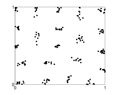
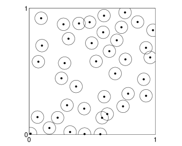
Figure 10: Left: Conditional Strauss process with $n=200$ points and parameters $\gamma=0.1$ and $r=0.2$. Right: Strauss process with $\beta=100$, $\gamma=0.1$, and $r=0.2$.

To generate the (unconditional) Strauss process using the Metropolis–Hastings sampler, the sampler needs to be able to “jump” between different dimensions $n$. The reversible jump sampler [15, 27] is an extension of the Metropolis–Hastings algorithm designed for this purpose. Instead of one transition density $q(\mathbf{y}\,|\,\mathbf{x})$, it requires a transition density for $n$, say $q(n\,|\,m)$, and for each $n$ a transition density $q(\mathbf{y}\,|\,\mathbf{x},n)$ to jump from $\mathbf{x}$ to an $n$-dimensional vector $\mathbf{y}$.

Given a current state $\mathbf{X}_{t}$ of dimension $m$, Step 1 of Algorithm 3.4 is replaced with

1. Generate a candidate dimension $n\sim q(n\,|\,m)$.

2. Generate an $n$-dimensional vector $\mathbf{Y}\sim q(\mathbf{y}\,|\,\mathbf{X}_{t},n)$.

And in Step 2 the acceptance ratio in (10) is replaced with

$$\alpha(\mathbf{x},\mathbf{y})=\min\left\{\frac{f(n,\mathbf{y})\,q(m\,|\,n)\,q(\mathbf{x}\,|\,\mathbf{y},m)}{f(m,\mathbf{x})\,q(n\,|\,m)\,q(\mathbf{y}\,|\,\mathbf{x},n)},\>1\right\}\;.$$ (12)

The $\mathrm{M}\mathrm{{\scriptstyle ATLAB}}$ program below implements a simple version of the reversible jump sampler, suggested in [12]. From a current state $\mathbf{x}$ of dimension $m$, a candidate dimension is chosen to be either $m+1$ or $m-1$, with equal probability. Thus, $q(m+1\,|\,m)=q(m-1\,|\,m)=1/2,m=1,2,\ldots.$ The first transition corresponds to the birth of a new point; the second to the death of a point. On the occasion of a birth, a candidate $\mathbf{Y}$ is generated by simply appending a uniform point on $[0,1]^{2}$ to $\mathbf{x}$. The corresponding transition density is therefore $q(\mathbf{y}\,|\,\mathbf{x},m)=1$. On the occasion of a death, the candidate $\mathbf{Y}$ is obtained from $\mathbf{x}$ by removing one of the points of $\mathbf{x}$ at random and uniformly. The transition density is thus $q(\mathbf{y}\,|\,\mathbf{x},m)=1/n(\mathbf{x})$. This gives the acceptance ratios:

• Birth:

  $$\alpha(\mathbf{x},\mathbf{y})=\min\left\{\frac{\beta^{n(\mathbf{y})}\gamma^{s(\mathbf{y})}\frac{1}{n(\mathbf{y})}}{\beta^{n(\mathbf{x})}\gamma^{s(\mathbf{x})}1},\>1\right\}=\min\{(\beta\gamma^{s(\mathbf{y})-s(\mathbf{x})})/n(\mathbf{y}),\>1\}\;.$$

• Death:

  $$\alpha(\mathbf{x},\mathbf{y})=\min\left\{\frac{\beta^{n(\mathbf{y})}\gamma^{s(\mathbf{y})}1}{\beta^{n(\mathbf{x})}\gamma^{s(\mathbf{x})}\frac{1}{n(\mathbf{x})}},\>1\right\}=\min\{(\gamma^{s(\mathbf{y})-s(\mathbf{x})}\,n(\mathbf{x}))/\beta,\>1\}\;.$$

r = 0.1; gam = 0.2; beta = 100; %parameters
n = 200; x = rand(n,2); %initial pp
K = 1000;
for i=1:K
    n = size(x,1);
    B = (rand < 0.5);
    if B %birth
        xnew = rand(1,2);
        y = [x;xnew];
        n = n+1;
    else %death
        y = setdiff(x,x(ceil(n*rand),:),’rows’);
    end
    if (max(max(y)) > 1 || min(min(y)) <0)
        alpha =0; %don’t accept a point outside the region
    elseif (numpairs(y,r) < numpairs(x,r))
        alpha =1;
    elseif B %birth
        alpha = beta*gam^(numpairs(y,r) - numpairs(x,r))/n;
    else  %death
        alpha = n*gam^(numpairs(y,r) - numpairs(x,r))/beta;
    end
    if (rand < alpha)
        x = y;
    end
    plot(x(:,1),x(:,2),’.’);
    axis([0,1,0,1]); refresh; pause(0.0001);

4 Wiener Surfaces

Brownian motion is one of the simplest continuous-time stochastic processes, and as such has found myriad applications in the physical sciences [20]. As a first step toward constructing Brownian motion we introduce the one-dimensional Wiener process $\{W_{t},t\in\mathbb{R}_{+}\}$, which can be viewed as a spatial process with a continuous index set on $\mathbb{R}_{+}$ and with a continuous state space $\mathbb{R}$.

4.1 Wiener Process

A one dimensional Wiener process is a stochastic process $\{W_{t},t\geqslant 0\}$ characterized by the following properties: (1) the increments of $W_{t}$ are stationary and normally distributed, that is, $W_{t}-W_{s}\sim{\sf N}(0,t-s)$ for all $t\geqslant s\geqslant 0$; (2) $W$ has independent increments, that is, for any $t_{1}<t_{2}\leqslant t_{3}<t_{4}$, the increments $W_{t_{4}}-W_{t_{3}}$ and $W_{t_{2}}-W_{t_{1}}$ are independent random variables (in other words, $W_{t}-W_{s},\;t>s$ is independent of the past history of $\{W_{u},\;0\leqslant u\leqslant s\}$); (3) continuity of paths, that is, $\{W_{t}\}$ has continuous paths with $W_{0}=0$.

The simplest algorithm for generating the process uses the Markovian (independent increments) and Gaussian properties of the Wiener process. Let $0=t_{0}<t_{1}<t_{2}<\dots<t_{n}$ be the set of distinct times for which simulation of the process is desired. Then, the Wiener process is generated at times $t_{1},\ldots,t_{n}$ via

$$W_{t_{k}}=\sum_{i=1}^{k}\sqrt{t_{k}-t_{k-1}}\;Z_{i},\quad k=1,\ldots,n\;,$$

where $Z_{1},\ldots,Z_{n}\stackrel{{\scriptstyle\text{iid}}}{{\sim}}{\sf N}(0,1)$. To obtain a continuous path approximation to the path of the Wiener process, one could use linear interpolation on the points $W_{t_{1}},\dots,W_{t_{n}}$. A realization of a Wiener process is given in the middle panel of Figure 11.

Given the Wiener process $W_{t}$, we can now define the $d$-dimensional Brownian motion process via

$$\widetilde{\mathbf{X}}_{t}=\boldsymbol{\mu}\,t+\Sigma^{1/2}\mathbf{W}_{t},\quad\mathbf{W}_{t}=(W_{t}^{(1)},\ldots,W_{t}^{(d)})^{\top},\quad t\geqslant 0\;,$$ (13)

where $W_{t}^{(1)},\ldots,W_{t}^{(d)}$ are independent Wiener processes and $\Sigma$ is a $d\times d$ covariance matrix. The parameter $\boldsymbol{\mu}\in\mathbb{R}^{d}$ is called the drift parameter and $\Sigma$ is called the diffusion matrix.

One approach to generalizing the Wiener process conceptually or to higher spatial dimensions is to use its characterization as a zero-mean Gaussian process (see Section 2.1) with continuous sample paths and covariance function $\text{Cov}(W_{t},W_{s})=\min\{t,s\}$ for $t,s>0$. Since $\frac{1}{2}\left(|t|+|s|-|t-s|\right)=\min\{t,s\}$, we can consider the covariance function $\frac{1}{2}\left(|t|+|s|-|t-s|\right)$ as a basis for generalization. The first generalization is obtained by considering a continuous zero-mean Gaussian process with covariance $\varrho(t,s)=\frac{1}{2}\left(|t|^{\alpha}+|s|^{\alpha}-|t-s|^{\alpha}\right)$, where $\alpha$ is a parameter such that $\alpha=1$ yields the Wiener process. This generalization gives rise to fractional Brownian motion discussed in the next section.

4.2 Fractional Brownian Motion

A continuous zero-mean Gaussian process $\{W_{t},t\geqslant 0\}$ with covariance function

$$\text{Cov}(W_{t},W_{s})=\frac{1}{2}\left(|t|^{\alpha}+|s|^{\alpha}-|t-s|^{\alpha}\right),\quad t,s\geqslant 0$$ (14)

is called fractional Brownian motion (fBm) with roughness parameter $\alpha\in(0,2)$. The process is frequently parameterized with respect to $H=\alpha/2$, in which case $H\in(0,1)$ is called the Hurst or self-similarity parameter. The notion of self-similarity arises, because fBm satisfies the property that the rescaled process $\{c^{-H}\,W_{c\,t},t\geqslant 0\}$ has the same distribution as $\{W_{t},t\geqslant 0\}$ for all $c>0$.

Generation of fBm on the uniformly spaced grid $0=t_{0}<t_{1}<t_{2}<\dots<t_{n}=1$ can be achieved by first generating the increment process $\{X_{1},X_{2},\ldots,X_{n}\}$, where $X_{i}=W_{i}-W_{i-1}$, and then delivering the cumulative sum

$$W_{t_{i}}=c^{H}\;\sum_{k=1}^{i}X_{k},\;i=1,\ldots,n,\quad c=1/n\;.$$

The increment process $\{X_{1},X_{2},\ldots,X_{n}\}$ is called fractional Gaussian noise and can be characterized as a discrete zero-mean stationary Gaussian process with covariance

$$\text{Cov}(X_{i},X_{i+k})=\frac{1}{2}\left(|k+1|^{\alpha}-2|k|^{\alpha}+|k-1|^{\alpha}\right),\quad k=0,1,2,\ldots$$

Since the fractional Gaussian noise is stationary, we can generate it efficiently using the circulant embedding approach in Section 2.2. First, we compute the first row $(r_{1},\ldots,r_{n+1})$ of the symmetric Toeplitz $(n+1)\times(n+1)$ covariance matrix $\Omega$ with elements $\Omega_{i+1,j+1}=\text{Cov}(X_{i},X_{j}),\;i,j=0,\ldots,n$. Second, we build the first row of the $2n\times 2n$ circulant matrix $\Sigma$, which embeds $\Omega$ in the upper left $(n+1)\times(n+1)$ corner. Thus, the first row of $\Sigma$ is given by $\mathbf{r}=(r_{1},\ldots,r_{n+1},r_{n},r_{n-1},\ldots,r_{2})$. We now seek a factorization of the form (3). Here, $\boldsymbol{\lambda}$ is the one-dimensional FFT of $\mathbf{r}$ defined as the linear transformation $\boldsymbol{\lambda}=F\mathbf{r}$ with $F_{j,k}=\exp(-2\pi\mathrm{i}jk/(2n))/\sqrt{2n},\;j,k=0,1,\ldots,2n-1$. Finally, the real and imaginary parts of the first $n+1$ components of $F^{*}\text{diag}(\sqrt{\boldsymbol{\lambda}})\mathbf{Z}$, where $\mathbf{Z}$ is a $2n\times 1$ complex valued Gaussian vector, yield two independent realizations of fractional Brownian noise. Figure 11 shows how the smoothness of fBm depends on the Hurst parameter. Note that $H=0.5$ corresponds to Wiener motion.

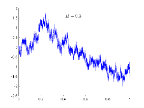
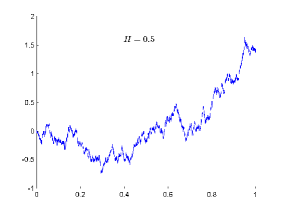
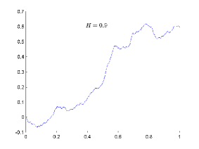
Figure 11: Fractional Brownian motion for different values of the Hurst parameter $H$. From left to right we have $H=0.3,0.5,0.9$.

The following $\mathrm{M}\mathrm{{\scriptstyle ATLAB}}$ code implements the circulant embedding method for fBm.

n=2^15; % grid points
H = 0.9; %Hurst parameter
r=nan(n+1,1); r(1) = 1;
for k=1:n
    r(k+1) = 0.5*((k+1)^(2*H) - 2*k^(2*H) + (k-1)^(2*H));
end
r=[r; r(end-1:-1:2)]; % first rwo of circulant matrix
lambda=real(fft(r))/(2*n); % eigenvalues
W=fft(sqrt(lambda).*complex(randn(2*n,1),randn(2*n,1)));
W = n^(-H)*cumsum(real(W(1:n+1))); % rescale
plot((0:n)/n,W);

4.3 Fractional Wiener Sheet in $\mathbb{R}^{2}$

A simple spatial generalization of the fractional Brownian motion is the fractional Wiener sheet in two dimensions. The fractional Wiener sheet process on the unit square is the continuous zero-mean Gaussian process $\{W_{\mathbf{t}},\>\mathbf{t}\in[0,1]^{2}\}$ with covariance function

$$\text{Cov}(W_{\mathbf{t}},W_{\mathbf{s}})=\frac{1}{4}(|s_{1}|^{\alpha}+|t_{1}|^{\alpha}-|s_{1}-t_{1}|^{\alpha})(|s_{2}|^{\alpha}+|t_{2}|^{\alpha}-|s_{2}-t_{2}|^{\alpha})\;,$$ (15)

which is simply a product form extension of (14). For the special case of $\alpha=1$, we can also write the covariance as $\text{Cov}(W_{\mathbf{t}},W_{\mathbf{s}})=\min\{t_{1},s_{1}\}\,\min\{t_{2},s_{2}\}$.

As in the one-dimensional case of fBm, we can consider the two-dimensional fractional Gaussian noise process $\{X_{i,j},\;i,j=1,\ldots,n\}$, which can be used to construct a fractional Wiener sheet on a uniformly spaced square grid via the cumulative sum

$$W_{t_{i},t_{j}}=n^{-2H}\sum_{k=1}^{i}\sum_{l=1}^{j}X_{k,l}\;,\quad i,j=1,\ldots,n\;.$$

Note that this process is self-similar in the sense that $(m\,n)^{-H}\sum_{k=1}^{m}\sum_{l=1}^{n}X_{k,l}$ has the same distribution as $X_{1,1}$ for all $m,n$, and $H$, see [22].

Generating a the two-dimensional fractional Gaussian noise process requires that we generate a zero-mean stationary Gaussian process with covariance [26]

$$\text{Cov}(X_{i,j},X_{i+k,j+l})=\frac{|k+1|^{\alpha}-2|k|^{\alpha}+|k-1|^{\alpha}}{2}\times\frac{|l+1|^{\alpha}-2|l|^{\alpha}+|l-1|^{\alpha}}{2}$$

for $k,l=0,1,\ldots,n$. We can thus proceed to generate this process using the circulant embedding method in Section 2.2. The generation of the Wiener sheet for $H=0.5$ is particularly easy since then all of the $X_{i,j}$ are independent standard normally distributed. Figure 12 shows realizations of fractional Wiener sheets for $H=\frac{1}{2}\alpha\in\{0.2,0.5,0.8\}$ with $n=2^{9}$.

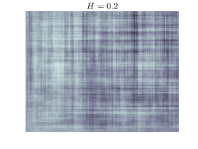
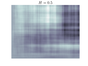
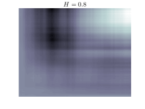
Figure 12: Fractional Wiener sheets with different Hurst parameter $H$.

Two objects which are closely related to $W_{\mathbf{t}}$ are the Wiener pillow and the Wiener bridge, which are zero-mean Gaussian processes on $[0,1]^{d}$ with covariance functions $\text{Cov}(W_{\mathbf{t}},W_{\mathbf{s}})=\prod_{i=1}^{d}(\min(t_{i},s_{i})-t_{i}s_{i})$ and $\prod_{i=1}^{d}\min(t_{i},s_{i})-\prod_{i=1}^{d}t_{i}s_{i}$, respectively.

4.4 Fractional Brownian Field

Fractional Brownian surface or field in two dimensions can be defined as the zero-mean Gaussian process $\{\widetilde{X}_{\mathbf{t}},\mathbf{t}\in\mathbb{R}^{2}\}$ with nonstationary covariance function

$$\text{Cov}(\widetilde{X}_{\mathbf{s}},\widetilde{X}_{\mathbf{t}})=\widetilde{\varrho}(\mathbf{s},\mathbf{t})=\|\mathbf{s}\|^{\alpha}+\|\mathbf{t}\|^{\alpha}-\|\mathbf{s}-\mathbf{t}\|^{\alpha}\;.$$ (16)

The parameter $H=\frac{\alpha}{2}\in(0,1)$ is the Hurst parameter controlling the roughness of the random field or surface. Contrast this isotropic generalization of the covariance (14) with the product form extension of the covariance in (15).

Generation of $\widetilde{X}_{\mathbf{t}}$ over a unit (quarter) disk in the first quadrant involves the following steps. First, we use Dietrich and Newsam’s method (Section 2.2) to generate a stationary Gaussian field $\breve{X}_{\mathbf{t}}$ with covariance function over the quarter disk $\{\mathbf{h}:\|\mathbf{h}\|\leqslant 1,\mathbf{h}>\mathbf{0}\}$

$$\breve{\varrho}(\mathbf{s},\mathbf{t})=c_{0}+c_{2}\|\mathbf{s}-\mathbf{t}\|^{2}-\|\mathbf{s}-\mathbf{t}\|^{\alpha}$$

for some constants $c_{0},c_{2}\geqslant 0$ whose selection will be discussed later. Once we have generated $\breve{X}_{\mathbf{t}}$, the process $\widetilde{X}_{\mathbf{t}}$ is obtained via the adjustment:

$$\widetilde{X}_{\mathbf{t}}=\breve{X}_{\mathbf{t}}-\breve{X}_{\mathbf{0}}+\sqrt{2c_{2}}\;\mathbf{t}^{\top}\mathbf{Z},\quad\mathbf{Z}=(Z_{1},Z_{2})^{\top},\quad Z_{1},Z_{2}\stackrel{{\scriptstyle\text{iid}}}{{\sim}}{\sf N}(0,1)\;.$$

It is straightforward to verify that the covariance structure of $\widetilde{X}_{\mathbf{t}}$ over the disk $\{\mathbf{h}:\|\mathbf{h}\|\leqslant 1,\mathbf{h}>\mathbf{0}\}$ is given by (16). It now remains to explain how we generate the process $\breve{X}_{\mathbf{t}}$. The idea is to generate the process on $[0,R]^{2},\,R\geqslant 1$ via the intrinsic embedding of Stein (see (5)) using the covariance function:

$$\psi(\mathbf{h})=\begin{cases}c_{0}+c_{2}\|\mathbf{h}\|^{2}-\|\mathbf{h}\|^{\alpha},&\|\mathbf{h}\|\leqslant 1\\ \frac{\beta(R-\|\mathbf{h}\|)^{3}}{\|\mathbf{h}\|},&1\leqslant\|\mathbf{h}\|\leqslant R\\ 0,&\|\mathbf{h}\|\geqslant R\end{cases},$$ (17)

where depending on the value of $\alpha$, the constants $R\geqslant 1,\beta\geqslant 0,c_{2}>0,c_{0}\geqslant 0$ are defined in Table 1.

	$0<\alpha\leqslant 1.5$	$1.5<\alpha<2$
$R$	1	2
$\beta$	0	$\frac{\alpha(2-\alpha)}{3R(R^{2}-1)}$
$c_{2}$	$\frac{1}{2}\alpha$	$\frac{\alpha-\beta(R-1)^{2}(R+2)}{2}$
$c_{0}$	$1-c_{2}$	$\beta(R-1)^{3}+1-c_{2}$

Table 1: Parameter values needed to ensure that (17) allows for a nonnegative circulant embedding.

Note that for $\alpha>1.5$, the parameters needed for a nonnegative embedding are more complex, because a covariance function that is smoother close to the origin has to be even smoother elsewhere. In particular, for $\alpha>1.5$ the choice of constants ensures that $\psi$ is twice continuously differentiable as a function of $\|\mathbf{h}\|$. Notice that while we generate the process $\widetilde{X}_{\mathbf{t}}$ over the square grid $[0,R]^{2}$, we are only interested in $\widetilde{X}_{\mathbf{t}}$ restricted inside the quarter disk with covariance $\breve{\varrho}(\mathbf{s},\mathbf{t})$. Thus, in order to reduce the computational effort, we would like to have $R\geqslant 1$ as close as possible to $1$. While the optimal choice $R=1$ guarantees a nonnegative embedding for all $\alpha\leqslant 1.5$, in general we need $R>1$ to ensure the existence of a minimal embedding for $\alpha>1.5$. The choice $R=2$ given in Table 1 is the most conservative one that guarantees a nonnegative circulant embedding for $\alpha>1.5$. Smaller values of $R$ that admit a nonnegative circulant embedding can be determined numerically [30, Table 1]. As a numerical example consider generating a fractional Brownian surface with $m=n=1000$ and for Hurst parameter $H\in(0.2,0.5,0.8)$. Figure 13 shows the effect of the parameter on the smoothness of the surface, with larger values providing a smoother surface.

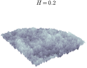
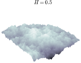
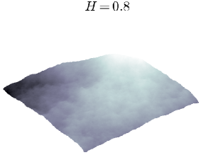
Figure 13: Fractional Brownian fields with different roughness parameter $\alpha=2H$.

We used the following $\mathrm{M}\mathrm{{\scriptstyle ATLAB}}$ code for the generation of the surfaces.

H=0.8;        % Hurst parameter
R=2;          % [0,R]^2 grid, may have to extract only  [0,R/2]^2
n=1000; m=n; % size of grid is m*n; covariance matrix is m^2*n^2
tx=[1:n]/n*R; ty=[1:m]/m*R; % create grid for field
Rows=zeros(m,n);
for i=1:n
    for j=1:m % rows of blocks of cov matrix
        Rows(j,i)=rho([tx(i),ty(j)],[tx(1),ty(1)],R,2*H);
    end
end
BlkCirc_row=[Rows, Rows(:,end-1:-1:2);
    Rows(end-1:-1:2,:), Rows(end-1:-1:2,end-1:-1:2)];
% compute eigen-values
lam=real(fft2(BlkCirc_row))/(4*(m-1)*(n-1));
lam=sqrt(lam);
% generate field with covariance given by block circular matrix
Z=complex(randn(2*(m-1),2*(n-1)),randn(2*(m-1),2*(n-1)));
F=fft2(lam.*Z);
F=F(1:m,1:n); % extract sub-block with desired covariance
[out,c0,c2]=rho([0,0],[0,0],R,2*H);
field1=real(F); field2=imag(F); % two independent fields
field1=field1-field1(1,1); % set field zero at origin
% make correction for embedding with a term c2*r^2
field1=field1 + kron(ty’*randn,tx*randn)*sqrt(2*c2);
[X,Y]=meshgrid(tx,ty);
field1((X.^2+Y.^2)>1)=nan;
surf(tx(1:n/2),ty(1:m/2),field1(1:n/2,1:m/2),’EdgeColor’,’none’)
colormap bone

The code uses the function rho.m, which implements the embedding (17).

function [out,c0,c2]=rho(x,y,R,alpha)
% embedding of covariance function on a [0,R]^2 grid
if alpha<=1.5 % alpha=2*H, where H is the Hurst parameter
    beta=0;c2=alpha/2;c0=1-alpha/2;
else % parameters ensure piecewise function twice differentiable
    beta=alpha*(2-alpha)/(3*R*(R^2-1));
    c2=(alpha-beta*(R-1)^2*(R+2))/2;
    c0=beta*(R-1)^3+1-c2;
end
% create continuous isotropic function
r=sqrt((x(1)-y(1))^2+(x(2)-y(2))^2);
if r<=1
    out=c0-r^alpha+c2*r^2;
elseif r<=R
    out=beta*(R-r)^3/r;
else
    out=0;
end

5 Spatial Levy Processes

Recall from Section 4.1 that the Brownian motion process (13) can be characterized as a continuous sample path process with stationary and independent Gaussian increments. The Lévy process is one of the simplest generalizations of the Brownian motion process, in cases where either the assumption of normality of the increments, or the continuity of the sample path is not suitable for modeling purposes.

5.1 Lévy Process

A $d$-dimensional Lévy process $\{\mathbf{X}_{t},t\in\mathbb{R}_{+}\}$ with $\mathbf{X}_{0}=0$ is a stochastic process with a continuous index set on $\mathbb{R}_{+}$ and with a continuous state space $\mathbb{R}^{d}$ defined by the following properties: (1) the increments of $\{\mathbf{X}_{t}\}$ are stationary, that is, $(\mathbf{X}_{t+s}-\mathbf{X}_{t})$ has the same distribution as $\mathbf{X}_{s}$ for all $t,s\geqslant 0$; (2) the increments of $\{\mathbf{X}_{t}\}$ are independent, that is, $\mathbf{X}_{t_{i}}-\mathbf{X}_{t_{i-1}},\;i=1,2,\ldots$ are independent for any $0\leqslant t_{0}<t_{1}<t_{2}<\cdots$; and (3) for any $\varepsilon>0$, we have $\mathbb{P}(\|\mathbf{X}_{t+s}-\mathbf{X}_{t}\|\geqslant\varepsilon)=0$ as $s\downarrow 0$.

From the definition it is clear that Brownian motion (13) is an example of a Lévy process, with normally distributed increments. Brownian motion is the only Lévy process with continuous sample paths. Other basic examples of Lévy processes include the Poisson process $\{N_{t},t\geqslant 0\}$ with intensity $\lambda>0$, where $N_{t}\sim{\sf Poi}(\lambda t)$ for each $t$, and the compound Poisson process defined via

$$\mathbf{J}_{t}=\sum_{k=1}^{N_{t}}\delta\mathbf{X}_{k},\quad N_{t}\sim{\sf Poi}(\lambda t)\;,$$ (18)

where $\delta\mathbf{X}_{1},\delta\mathbf{X}_{2},\ldots$ are iid random variables, independent of $\{N_{t},t\geqslant 0\}$. We can more generally express $\mathbf{J}_{t}$ as $\mathbf{J}_{t}=\int_{0}^{t}\int_{\mathbb{R}^{d}}\mathbf{x}\,N(\text{d}s,\text{d}\mathbf{x})$, where $N(\text{d}s,\text{d}\mathbf{x})$ is a Poisson random counting measure on $\mathbb{R}_{+}\times\mathbb{R}^{d}$ (see Section 3.1) with mean measure $\mathbb{E}[N([0,t]\times A)],\;A\in{\cal E},$ equal to the expected number of jumps of size $A$ in the interval $[0,t]$.

A crucial property of Lévy processes is infinite divisibility. In particular, if we define $\mathbf{Y}_{j}^{(n)}=\mathbf{X}_{j\,t/n}-\mathbf{X}_{(j-1)\,t/n}$, then using the stationarity and independence properties of the Lévy process, we obtain that for each $n\geqslant 2$ the $\{\mathbf{Y}_{1}^{(n)}\}$ are independent and identically distributed random variables with the same distribution as $\mathbf{X}_{t/n}$. Thus, for a fixed $t$ we can write

$$\mathbf{X}_{t}\sim\mathbf{Y}_{1}^{(n)}+\cdots+\mathbf{Y}_{n}^{(n)}\;,\textrm{ for any }n\geqslant 2\;,$$ (19)

and hence by definition the random vector $\mathbf{X}_{t}$ is infinitely divisible (for a fixed $t$). The Lévy–Khintchine theorem [29] gives the most general form of the characteristic function of an infinitely divisible random variable. Specifically, the logarithm of the characteristic function of $\mathbf{X}_{t}$ (the so-called characteristic exponent) is of the form

$$\ln\mathbb{E}[\text{e}^{\mathrm{i}\,\mathbf{s}^{\top}\mathbf{X}_{t}}]=\mathrm{i}\,t\,\mathbf{s}^{\top}\boldsymbol{\mu}-\frac{1}{2}\,t\,\mathbf{s}^{\top}\Sigma\mathbf{s}+t\int_{\mathbb{R}^{d}}\left(\text{e}^{\mathrm{i}\,\mathbf{s}^{\top}\mathbf{x}}-1-\mathrm{i}\,\mathbf{s}^{\top}\mathbf{x}\,\text{I}_{\{\|\mathbf{x}\|\leqslant 1\}}\right)\nu(\text{d}\mathbf{x})\;,$$ (20)

for some $\boldsymbol{\mu}\in\mathbb{R}^{d}$, covariance matrix $\Sigma$ and measure $\nu$ such that $\nu(\{\mathbf{0}\})=0$,

$$\int_{\|\mathbf{x}\|>1}\!\!\!\nu(\text{d}\mathbf{x})<\infty\;\textrm{ and }\int_{\|\mathbf{x}\|\leqslant 1}\|\mathbf{x}\|^{2}\nu(\text{d}\mathbf{x})<\infty\;\Leftrightarrow\int_{\mathbb{R}^{d}}\min\{1,\|\mathbf{x}\|^{2}\}\nu(\text{d}\mathbf{x})<\infty\;.$$ (21)

The triplet $(\boldsymbol{\mu},\Sigma,\nu)$ is referred to as the characteristic triplet defining the Lévy process. The measure $\nu$ is referred to as the Lévy measure. Note that for a general $\nu$ satisfying (21), the integral $\int_{\mathbb{R}^{d}}\big{(}\text{e}^{\mathrm{i}\,\mathbf{s}^{\top}\mathbf{x}}-1\big{)}\nu(\text{d}\mathbf{x})$ in (20) does not converge separately. In this sense $\mathrm{i}\,\mathbf{s}^{\top}\mathbf{x}\,\text{I}_{\{\|\mathbf{x}\|\leqslant 1\}}$ in (20) serves the purpose of enforcing convergence under the very general integrability condition (21). However, if in addition to (21) the measure $\nu$ satisfies $\int_{\mathbb{R}^{d}}\min\{1,\|\mathbf{x}\|\}\nu(\text{d}\mathbf{x})<\infty$ and $\nu(\mathbb{R}^{d})<\infty$, then the integral in (20) can be separated as $t\int_{\mathbb{R}^{d}}(\text{e}^{\mathrm{i}\,\mathbf{s}^{\top}\mathbf{x}}-1)\nu(\text{d}\mathbf{x})-\mathrm{i}\,t\,\mathbf{s}^{\top}\int_{\|\mathbf{x}\|\leqslant 1}\mathbf{x}\,\nu(\text{d}\mathbf{x})$, and the characteristic exponent simplifies to

$$\underbrace{\mathrm{i}\,t\,\mathbf{s}^{\top}\boldsymbol{\mu}^{*}-\frac{1}{2}\,t\,\mathbf{s}^{\top}\Sigma\,\mathbf{s}}_{\textrm{Brownian motion term}}+\underbrace{t\int_{\mathbb{R}^{d}}\left(\text{e}^{\mathrm{i}\,\mathbf{s}^{\top}\mathbf{x}}-1\right)\nu(\text{d}\mathbf{x})}_{\textrm{Poisson process term}},$$

where $\boldsymbol{\mu}^{*}=\boldsymbol{\mu}-\int_{\|\mathbf{x}\|\leqslant 1}\mathbf{x}\,\nu(\text{d}\mathbf{x})$. We can now recognize this characteristic exponent as the one corresponding to the process $\{\mathbf{X}_{t}\}$ defined by $\mathbf{X}_{t}=t\boldsymbol{\mu}^{*}+\Sigma^{1/2}\mathbf{W}_{t}+\mathbf{J}_{t}$, where $t\boldsymbol{\mu}^{*}+\Sigma^{1/2}\mathbf{W}_{t}$ defines a Brownian motion (see (13)) and $\{\mathbf{J}_{t}\}$ is a compound Poisson process (18) with jump size distribution $\delta\mathbf{X}_{1}\sim\nu(\text{d}\mathbf{x})/\lambda$. Thus, $\nu(\text{d}\mathbf{x})$ can be interpreted as the intensity of the jump sizes in this particular Lévy process. In a similar way, it can be shown that the most general Lévy process $\{\mathbf{X}_{t}\}$ with characteristic triplet $(\boldsymbol{\mu},\Sigma,\nu)$ and integrability condition (21) can be represented as the limit in probability of a process $\{\mathbf{X}_{t}^{(\varepsilon)}\}$ as $\varepsilon\downarrow 0$, where $\mathbf{X}_{t}^{(\varepsilon)}$ has the Lévy-Itô decomposition

$$\mathbf{X}_{t}^{(\varepsilon)}=t\boldsymbol{\mu}+\Sigma^{1/2}\mathbf{W}_{t}+\mathbf{J}_{t}+\left(\mathbf{J}_{t}^{(\varepsilon)}-t\int_{\varepsilon<\|\mathbf{x}\|\leqslant 1}\,\mathbf{x}\,\nu(\text{d}\mathbf{x})\right)$$ (22)

with the following independent components:

1. $\{t\boldsymbol{\mu}+\Sigma^{1/2}\mathbf{W}_{t}\}$ is the Brownian motion (13), which corresponds to the $\mathrm{i}\,t\,\mathbf{s}^{\top}\boldsymbol{\mu}-\frac{1}{2}\,t\,\mathbf{s}^{\top}\Sigma\,\mathbf{s}$ part of (20).

2. $\{\mathbf{J}_{t}\}$ is a compound Poisson process of the form (18) with $\lambda=\int_{\|\mathbf{x}\|>1}\nu(\text{d}\mathbf{x})$ and increment distribution $\delta\mathbf{X}_{1}\sim\nu(\text{d}\mathbf{x})/\lambda$ over $\|\mathbf{x}\|>1$, which corresponds to the $\int_{0}^{t}\int_{\|\mathbf{x}\|>1}(\text{e}^{\mathrm{i}\,\mathbf{s}^{\top}\mathbf{x}}-1)\nu(\text{d}\mathbf{x})\,\text{d}t$ part in the characteristic exponent (20).

3. $\{\mathbf{J}_{t}^{(\varepsilon)}\}$ is a compound Poisson process with $\lambda=\nu(\varepsilon<\|\mathbf{x}\|\leqslant 1)$ and increment distribution $\nu(\text{d}\mathbf{x})/\lambda$ over $\varepsilon<\|\mathbf{x}\|\leqslant 1$, so that the compensated compound Poisson process $\{\mathbf{J}_{t}^{(\varepsilon)}-t\int_{\varepsilon<\|\mathbf{x}\|\leqslant 1}\mathbf{x}\,\nu(\text{d}\mathbf{x})\}$ corresponds to the $\int_{0}^{t}\int_{\|\mathbf{x}\|\leqslant 1}\left(\text{e}^{\mathrm{i}\,\mathbf{s}^{\top}\mathbf{x}}-1-\mathrm{i}\,\mathbf{s}^{\top}\mathbf{x}\right)\nu(\text{d}\mathbf{x})\,\text{d}t$ part of (20) in the limit $\varepsilon\downarrow 0$.

The Lévy–Itô decomposition immediately suggests an approximate generation method — we generate $\{\mathbf{X}_{t}^{(\varepsilon)}\}$ in (22) for a given small $\varepsilon$, where the Brownian motion part is generated via the methods in Section 4.1 and the compound Poisson process (18) in the obvious way. We are thus throwing away the very small jumps of size less than $\varepsilon$. For $d=1$ it can then be shown [1] that the error process $\{X_{t}-X_{t}^{(\varepsilon)}\}$ for this approximation is a Lévy process with characteristic triplet $(0,0,\nu(\text{d}x)\text{I}_{\{|x|<\varepsilon\}})$ and variance $\text{Var}(X_{t}-X_{t}^{(\varepsilon)})=t\int_{-\varepsilon}^{\varepsilon}x^{2}\nu(\text{d}x)$.

A given approximation $\mathbf{X}_{t}^{(\varepsilon_{n})}$ can always be further refined by adding smaller jumps of size $[\varepsilon_{n+1},\varepsilon_{n}]$ to obtain:

$$\mathbf{X}_{t}^{(\varepsilon_{n+1})}=\mathbf{X}_{t}^{(\varepsilon_{n})}+\mathbf{J}_{t}^{(\varepsilon_{n+1})}-t\int_{\varepsilon_{n+1}<\|\mathbf{x}\|\leqslant\varepsilon_{n}}\mathbf{x}\,\nu(\text{d}\mathbf{x})\;,\quad\varepsilon_{n}>\varepsilon_{n+1}>0\;,$$

where the compound Poisson process $\{\mathbf{J}_{t}^{(\varepsilon_{n+1})}\}$ has increment distribution given by $\nu(\text{d}\mathbf{x})/\nu(\varepsilon_{n+1}<\|\mathbf{x}\|\leqslant\varepsilon_{n})$ for all $\varepsilon_{n+1}<\|\mathbf{x}\|\leqslant\varepsilon_{n}$. For a more sophisticated method of refining the approximation see [1].

As an example consider the Lévy process $\{X_{t}\}$ with characteristic triplet $(\mu,0,\nu)$, where $\nu(\text{d}x)=\alpha\,\text{e}^{-x}/x\,\text{d}x$ for $\alpha,x>0$ and $\mu=\int_{|x|\leqslant 1}x\,\nu(\text{d}x)=\alpha(1-\text{e}^{-1})$. Here, in addition to (21), the infinite measure $\nu$ satisfies the stronger integrability condition $\int_{\mathbb{R}}\min\{1,|x|\}\nu(\text{d}x)<\infty$ and hence we can write $X_{t}=t\mu-t\int_{|x|\leqslant 1}x\,\nu(\text{d}x)+\int_{0}^{t}\int_{\mathbb{R}}x\,N(\text{d}s,\text{d}x)=\int_{0}^{t}\int_{\mathbb{R}_{+}}x\,N(\text{d}s,\text{d}x)$, where $\mathbb{E}[N(\text{d}s,\text{d}x)]=\text{d}s\,\nu(\text{d}x)$.

The leftmost panel of Figure 14 shows an outcome of the approximation $X_{t}^{(\varepsilon_{1})}$ in (22) over $t\in[0,1]$ for $\varepsilon_{1}=1$ and $\alpha=10$. The middle and rightmost panels show the refinements $X_{t}^{(\varepsilon_{2})}$ and $X_{t}^{(\varepsilon_{3})}$, respectively, where $(\varepsilon_{1},\varepsilon_{2},\varepsilon_{3})=(1,0.1,0.001)$. Note that the refinements add finer and finer jumps to the path.

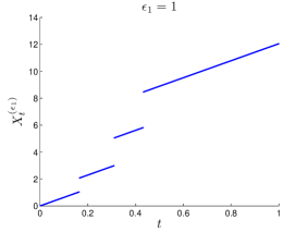
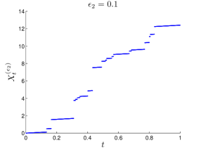
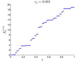
Figure 14: Approximate gamma process realizations obtained by throwing away jumps smaller than $\varepsilon_{i}$.

This process is called a gamma process and can be generated more simply using the fact that the increments $\{X_{jt/n}-X_{(j-1)t/n}\}$ have a known gamma distribution [19, Page 212]. The gamma process is an example of an increasing Lévy process (that is, $X_{t}\geqslant X_{s}$ almost surely for all $t\geqslant s$) called a Lévy subordinator. A Lévy subordinator $\{X_{t},t\geqslant 0\}$ has characteristic triplet $(\mu,0,\nu)$ satisfying the positive jump property $\nu((-\infty,0])=0$ and the positive drift property $0\leqslant\mu-\int_{0}^{1}x\nu(\text{d}x)<\infty$.

5.2 Lévy Sheet in $\mathbb{R}^{2}$

One way of generalizing the Lévy process to the spatial case is to insist on the preservation of the infinite divisibility property. In this generalization, a spatial Lévy process or simply a Lévy sheet $\{X_{\mathbf{t}},\mathbf{t}\in\mathbb{R}^{2}\}$ possesses the property that $(X_{\mathbf{t}_{1}},\ldots,X_{\mathbf{t}_{n}})$ is infinitely divisible for all indexes $\mathbf{t}_{1},\ldots,\mathbf{t}_{n}\in\mathbb{R}^{2}$ and any integer $n$ (see (19)). To construct such an infinitely divisible process, consider stochastic integration with respect to a random infinitely divisible measure $\Lambda$ defined as the stochastic process $\{\Lambda(A),\;A\in{\cal E}\}$ with the following properties:

1. For any set $A\in{\cal E}$ the random variable $\Lambda(A)$ has an infinitely divisible distribution with $\Lambda(\emptyset)=0$ almost surely.

2. For any disjoint sets $A_{1},A_{2},\ldots\in{\cal E}$, the random variables $\Lambda(A_{1}),\Lambda(A_{2}),\ldots$ are independent and $\Lambda(\cup_{i}A_{i})=\sum_{i}\Lambda(A_{i})$.

An example of a random infinitely divisible measure is the Poisson random measure (6) in Section 3.1. As a consequence of the independence and infinite divisibility properties, the characteristic exponent of $\Lambda(A),\;A\in{\cal E}$ has the Lévy–Khintchine representation (20):

$$\ln\mathbb{E}[\text{e}^{\mathrm{i}\,s\Lambda(A)}]=\mathrm{i}\,s\,\widetilde{\mu}(A)-\frac{1}{2}\,s^{2}(\widetilde{\sigma}(A))^{2}+\int_{\mathbb{R}}\left(\text{e}^{\mathrm{i}\,sx}-1-\mathrm{i}\,s\,x\,\text{I}_{\{|x|\leqslant 1\}}\right)\widetilde{\nu}(\text{d}x,A)\;,$$

where $\widetilde{\mu}$ is an additive set function, $\widetilde{\sigma}$ is a measure on the Borel sets ${\cal E}$, the measure $\widetilde{\nu}(\cdot,A)$ is a Lévy measure for each fixed $A\in{\cal E}$ (so that $\widetilde{\nu}(\{0\},A)=0$ and $\int_{\mathbb{R}}\min\{1,x^{2}\}\widetilde{\nu}(\text{d}x,A)<\infty$), and $\widetilde{\nu}(\text{d}x,\cdot)$ is a Borel measure for each fixed $\text{d}x$. For example, $X_{t}=\Lambda((0,t])$ defines a one-dimensional Lévy process.

We can then construct a Lévy sheet $\{X_{\mathbf{t}},\mathbf{t}\in\mathbb{R}^{2}\}$ via the stochastic integral

$$X_{\mathbf{t}}=\int_{\mathbb{R}^{d}}\kappa_{\mathbf{t}}(\mathbf{x})\,\Lambda(\text{d}\mathbf{x}),\quad\mathbf{t}\in\mathbb{R}^{2}\;,$$ (23)

where $\kappa_{\mathbf{t}}:\mathbb{R}^{d}\rightarrow\mathbb{R}$ is a Hölder continuous kernel function for all $\mathbf{t}\in\mathbb{R}^{2}$, which is integrable with respect to the random infinitely divisible measure $\Lambda$. Thus, the Lévy sheet (23) is a stochastic integral with a deterministic kernel function as integrand (determining the spatial structure) and a random infinitely divisible measure as integrator [16].

Consider simulating the Lévy sheet (23) over $\mathbf{t}\in[0,1]^{2}$ for $d=2$. Truncate the region of integration to a bounded domain, say $[0,1]^{2}$, so that $\kappa_{\mathbf{t}}(\mathbf{x})=0$ for each $\mathbf{x}\not\in[0,1]^{2}$ and $\mathbf{t}\in[0,1]^{2}$. Then, one way of simulating $\{X_{\mathbf{t}},\mathbf{t}\in[0,1]^{2}\}$ is to consider the approximation

$$X_{\mathbf{t}}^{(n)}=\sum_{i=0}^{n-1}\sum_{j=0}^{n-1}\kappa_{\mathbf{t}}(i/n,j/n)\;\Lambda(\triangle_{i,j}),\quad\triangle_{i,j}\equiv\left[\frac{i}{n},\frac{i+1}{n}\right]\times\left[\frac{j}{n},\frac{j+1}{n}\right]\;,$$ (24)

where all $\Lambda(\triangle_{i,j})$ are independent infinitely divisible random variables with characteristic triplet $(\widetilde{\mu}(\triangle_{i,j}),\widetilde{\sigma}(\triangle_{i,j}),\widetilde{\nu}(\,\cdot\,,\triangle_{i,j}))$. Under some technical conditions [16], it can be shown that $X_{\mathbf{t}}^{(n)}$ converges to $X_{\mathbf{t}}$ in probability as $n\uparrow\infty$.

As an example, consider generating (24) on the square grid $\{(i/m,j/m),\;i,j=0,\ldots,m-1\}$ with the kernel function

$$\kappa_{\mathbf{t}}(x_{1},x_{2})=(r^{2}-\|\mathbf{x}-\mathbf{t}\|^{2})\;\text{I}_{\{\|\mathbf{x}-\mathbf{t}\|\leqslant r\}},\quad\mathbf{t}\in[0,1]^{2}\;,$$

and $\Lambda(\triangle_{i,j})\stackrel{{\scriptstyle\text{iid}}}{{\sim}}{\sf Gamma}(\alpha|\triangle_{i,j}|,\beta),\;|\triangle_{i,j}|=1/n^{2}$ for all $i,j$, where ${\sf Gamma}(\alpha,\beta)$ denotes the density of the gamma distribution with pdf $\beta^{\alpha}x^{\alpha-1}\text{e}^{-\beta x}/\Gamma(\alpha),$ $x\geqslant 0$. The corresponding limiting process $\{X_{\mathbf{t}}\}$ is called a gamma Lévy sheet. Figure 15 shows realizations of (24) for $m=n=100$ and $r=0.05,\;\alpha=\beta\in\{10^{2},10^{5}\}$, so that we have the scaling $\mathbb{E}[\Lambda(\triangle_{i,j})]=\alpha/(\beta\,n^{2})=1/n^{2}$.

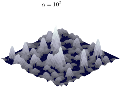
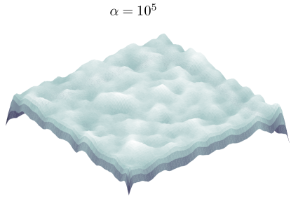
Figure 15: Gamma Lévy random sheet realizations for different values of the shape parameter $\alpha$.

Note that the sheet exhibits more bumps for smaller values of $\alpha$ than for large values of $\alpha$. For a method of approximately generating (23) using wavelets see [16].

Acknowledgement

This work was supported by the Australian Research Council under grant number DP0985177.

References

- [1] S. Asmussen and J. Rosiński. Approximations of small jumps of Lévy processes with a view towards simulation. Journal of Applied Probability, 38(2):482–493, 2001.
- [2] A. Baddeley. Spatial Point Processes and their Applications. Springer Lecture Notes in Mathematics (1892), 2007.
- [3] A. Baddeley, P. Gregori, J. Mateu, R. Stoica, and D. Stoyan. Case Studies in Spatial Point Process Modeling. Springer Lecture Notes in Statistics (185), 2006.
- [4] S. Barnett. Matrices, Methods and Applications. Oxford Applied Mathematics and Computing Sciences Series, 1990.
- [5] T. Brereton, D. P. Kroese, O. Stenzel, V. Schmidt, and G. Baumier. Efficient simulation of charge transport in deep-trap media. In C. Laroque, J. Himmelspach, R. Pasupathy, O. Rose, and A. M. Uhrmacher, editors, Proceedings of the 2012 Winter Simulation Conference, 2012.
- [6] A. Brix. Generalized gamma measures and shot-noise cox processes. Advances in Applied Probability, 31:929–953, 1999.
- [7] G. Chan and A. T. A. Wood. Simulation of stationary Gaussian vector fields. Statistics and Computing, 9:265–268, 1999.
- [8] D. Cox. Some statistical methods connected with series of events. Journal of the Royal Statistical Society, B, 17(24):129–164, 1955.
- [9] D. J. Daley and D. Vere-Jones. An Introduction to the Theory of Point Processes Volumes 1 and 2. Springer Series in Statistics, 2003.
- [10] C. R. Dietrich and G. N. Newsam. Fast and exact simulation of stationary Gaussian processes through circulant embedding of the covariance matrix. SIAM Journal on Scientific Computing, 18(4):1088–1107, 1997.
- [11] P. J. Diggle. Statistical Analysis of Spatial Point Patterns. Oxford University Press, London, New York, 2003.
- [12] Charles J. Geyer and Jesper M ller. Simulation procedures and likelihood inference for spatial point processes. Scandinavian Journal of Statistics, 21(4):pp. 359–373, 1994.
- [13] T. Gneiting, H. Seveikova, D. B. Percival, M. Schlather, and Y. Jiang. Fast and exact simulation of large Gaussian lattice systems in : Exploring the limits. Journal of Computational and Graphical Statistics, 15(3):483–501, 2006.
- [14] G. H. Golub and C. F. Van Loan. Matrix computations. Johns Hopkins University Press, third edition, 1996.
- [15] P. J. Green. Reversible jump Markov chain Monte Carlo computation and Bayesian model determination. Biometrika, 82(4):711–732, 1995.
- [16] W. Karcher, H.-P. Scheffler, and E. Spodarev. Simulation of infinitely divisible random fields. Communications in Statistics – Simulation and Computation, 42:215–246, 2013.
- [17] F. P. Kelly and B. D. Ripley. A note on Strauss’s model for clustering. Biometrika, 63(2):357–360, 1976.
- [18] M. Kendall and J. K. Ord. Time Series. Oxford University Press, Oxford, third edition, 1990.
- [19] D. P. Kroese, T. Taimre, and Z. I. Botev. Handbook of Monte Carlo Methods. Wiley, New Jersey, 2011.
- [20] G. F. Lawler. Introduction to Stochastic Processes. Chapman & Hall/CRC, FL, 2006.
- [21] J. Møller. Shot noise cox process. Advances in Applied Probability, 35(3):614–640, 2003.
- [22] B. B. Mandelbrot and J. W. van Ness. Fractional Brownian motions, fractional noises and applications. SIAM Review, 10(4):422–437, 1968.
- [23] B. Matérn. Spatial variation. Meddelanden från Statens Skogsforskningsinstitut, 49:1–144, 1960.
- [24] J. Møller and R. P. Waagepetersen. Statistical Inference and Simulation for Spatial Point Processes. Chapman & Hall/CRC, 2004.
- [25] J. Neyman and E. L. Scott. Statistical approach to problems of cosmology. Journal of the Royal Statistical Society. Series B (Methodological), 20(1):1–43, 1958.
- [26] H. Qian, G. M. Raymond, and J. B. Bassingthwaighte. On two-dimensional fractional Brownian motion and fractional Brownian random field. Journal of Physics A: Mathematical and General, 31(28), 1998.
- [27] C. P. Robert and G. Casella. Monte Carlo Statistical Methods. Springer-Verlag, New York, second edition, 2004.
- [28] H. Rue and L. Held. Gaussian Markov Random Fields: Theory and Applications. Chapman & Hall, London, 2005.
- [29] K. Sato. Lévy Processes and Infinitely Divisible Distributions. Cambridge University Press, Cambridge, 1999.
- [30] M. L. Stein. Fast and exact simulation of fractional Brownian motion. Journal of Computational and Graphical Statistics, 11(3):587–599, 2002.
- [31] O. Stenzel, D. P. Kroese D. Westhoff, I. Manke, and V. Schmidt. Graph-based simulated annealing: A hybrid approach to stochastic modeling of complex microstructures. submitted, 2012.
- [32] D. J. Strauss. Analysing binary lattice data with the nearest-neighbor property. Journal of Applied Probability, 12(4):702–712, 1975.
- [33] R. H. Swendsen and J.-S. Wang. Nonuniversal critical dynamics in Monte Carlo simulations. Physical Review Letters, 58(2):86–88, 1987.
- [34] A.T.A. Wood and G. Chan. Simulation of stationary Gaussian process in . Journal of Computational and Graphical Statistics, 3:409–432, 1994.