Probing the dynamic interference in molecular high-order harmonic generation through Bohmian trajectories

Abstract

By using Bohmian trajectory method, we investigate the dynamic interference in diatomic molecular high-order harmonic generation progress. It is demonstrated that the main characteristics of the molecular harmonic spectrum can be well reproduced by only two Bohmain trajectories which are located respectively at the two ions. This is because these two localized trajectories can receive and store the whole collision information coming from all of the other recollision trajectories. Therefore, the amplitudes and frequencies of these two trajectories represent the intensity and frequency distribution of the harmonic generation. Moreover, the interference between these two trajectories shows a dip in the harmonic spectrum, which indicates the molecular structure information.

When atoms and molecules are irradiated by an intense laser pulse, high-order harmonics of the laser’s frequency may be generated 1 ; 2 ; 3 ; 4 . The mechanism of high-order harmonic generation (HHG) is the recombination of the ionized electron with its parent ion in the laser field 5 ; 6 . HHG offers us a new way to detect the microscopic process with sub-angstrom spatial and attosecond temporal resolution 7 ; 8 ; 9 . HHG can also be applied to imaging the molecular orbitals 10 ; 11 ; 12 , probing the electronic or nuclear dynamical behavior with attosecond resolution 13 ; 14 ; 15 .

The response of single atom or molecule of HHG has been studied theoretically by using numerical solution of time-dependent schrödinger equation (TDSE) 16 ; 17 . The TDSE calculation can provide an accurate result to simulate the experiment measurement. However, it is difficult to extract the dynamic information of the HHG process from the time-dependent wavefunction and to make clear the physical mechanism behind the process. To overcome this difficulty, one can adopt the Bohmian trajectory(BT) scheme. Recently, this scheme has been used in the research on the interaction between matter and strong field. For example, by using this method, Takemoto et al. 18 investigated the attosecond electron dynamics of molecular ion, and Lai et al. 19 studied the correspondence between the quantum and classical processes in the strong field ionization. Furthermore, this scheme has been successfully applied to investigate the atomic HHG processes 19 ; 20 ; 21 . It is found that the calculation of the atomic HHG by solving the TDSE agrees well with the result by the BT scheme 21 .

In this work, the BT method is applied to study the dynamic interference process in the molecular HHG processes. For the HHG of small linear molecules, there is the minima in the harmonic spectra due to the interference of many atomic centers 22 ; 23 ; 24 ; 25 ; 26 ; 27 . This minima in the molecular HHG spectrum was firstly predicted theoretically by Lein et al. 16 ; 17 and confirmed experimentally by Kanai et al. 23 . The interference structure changes with the internuclear distance, the symmetry of molecular orbit, and multi-orbit effect 27 ; 28 . Thus it is necessary to make clear the physical mechanism behind the interference structure in the molecular HHG spectrum.

To understand the interference mechanism, we investigate the HHG of H${}_{2}^{+}$ molecular ion by using the BT scheme. It is found that the HHG can be reproduced qualitatively by using only two BTs whose initial positions are located at the two atomic centers respectively in the molecular ion. More importantly, the accurate interference structure in the molecular HHG spectrum can be illustrated through the dynamic analysis of the Bohmian particles’s acceleration. These Bohmian particles play the role as an ’antenna’ which can well reflect the dynamic information about the electron in the molecule.

I Theoretical methods

We take the electron probability density as a fluid, and its flow can be analyzed by the Bohmian mechanics of many Bohmian particles whose trajectories are guided by the quantum wavefunction 17 ; 29 ; 30 ; 31 . The quantum wavefunction $\psi(x,t)$ was obtained from the numerical solution of the one-dimensional TDSE (atomic units are used throughout this paper, unless otherwise stated): $i{\partial\psi(x,t)}{/{\partial t}}=H\psi(x,t)$, where $H=-{\partial}^{2}/(2\partial{x}^{2})+V(x,R,t)$ is the Hamtonian of the H${}_{2}^{+}$ molecular ion. Here $R$ is the distance between two protons, and $x$ is electronic coordinate in the molecular frame. Under dipole approximation and in length gauge, the time-dependent potential is $V(r,R,t)=V(x,R)+E(t)\cdot x$, where the soft-core potential $V(x,R)=-1/\sqrt{{{(x-R/2)}^{2}}+\alpha}-1/\sqrt{{{(x+R/2)}^{2}}+\alpha}$ is chosen to represent the interaction between the electron and the nuclei, where $\alpha$ is the soft core parameter. The laser-electron interaction potential is $E(t)\cdot x$, where the laser’s electric field is $E{\rm{(}}t{\rm{)=}}{E_{0}}f{\rm{(}}t{\rm{)}}\sin{\rm{(}}\omega t{\rm{)}}{\rm{}}$ with $\omega$ and $E_{0}$ being the frequency and peak amplitude of the laser pulse, respectively. The envelope of the laser’s electric field is $f(t)=\exp[-4\ln 2{\left({(t-T/2)/\sigma}\right)^{2}}]$ with the total width being $T=400$.

The TDSE are solved numerically using symmetrically splitting fast Fourier transformation scheme 32 ; 33 . By using the time-dependent wavefunction, the BTs $\left\{x_{k}(t)|k=1,...,N_{Tra}\right\}$ are propagated by solving the equation:

$${\dot{x}_{k}}(t)={\mathop{\rm Im}\nolimits}\left[{\frac{1}{{\psi(x,t)}}\frac{\partial}{{\partial x}}\psi(x,t){|_{x={x_{k}(t)}}}}\right].$$ (1)

The initial positions of the Bohmian particles are selected by the electron probability density of the ground state of H${}_{2}^{+}$, and for each trajectory we assign the same weight. The following positions of these Bohmian particles are calculated from the integration of Eq. (1) 28 . Furthermore, one can obtain the acceleration $a_{k}(t)=\ddot{x}_{k}(t)$ of the Bohmian particles by taking the derivative of Eq. (1). It should be noticed, in classical viewpoint, that the square of the particle’s acceleration is proportional to the instantaneous power of the radiation. Hence the harmonic spectrum of each particle can be obtained by using the Fourier transformation scheme:

$$P_{k}(\omega)={\left|{\frac{1}{{{t_{f}}-{t_{i}}}}\frac{1}{\omega^{2}}\int_{{t_{i}}}^{{t_{f}}}{a_{k}(t){e^{-i\omega t}}dt}}\right|^{2}}{\rm{,}}$$ (2)

where $t_{i}$ and $t_{f}$ are the initial and final instants of the laser pulse, respectively. The whole HHG of the molecular ion can be calculated from the Fourier transform of the acceleration of the total Bohmian trajectories :

$$P(\omega)={\left|{\frac{1}{{{t_{f}}-{t_{i}}}}\frac{1}{\omega^{2}}\int_{{t_{i}}}^{{t_{f}}}{a_{\rm BT}(t){e^{-i\omega t}}dt}}\right|^{2}}{\rm{,}}$$ (3)

where $a_{\rm BT}(t)=\sum_{k=1}^{N_{\rm Tra}}{a_{k}(t)/N_{\rm Tra}}$.

For the purpose of comparison, we also calculated the HHG from TDSE using the time dependent acceleration dipole:

$$P(\omega)={\left|{\frac{1}{{{t_{f}}-{t_{i}}}}\frac{1}{\omega^{2}}\int_{{t_{i}}}^{{t_{f}}}{a(t){e^{-i\omega t}}dt}}\right|^{2}}{\rm{,}}$$ (4)

where

$$a(t)=\left\langle{\psi(x,t)\left|{\frac{{dV(x,R)}}{{dx}}-E(t)}\right|\psi(x,t)}\right\rangle.$$ (5)

II Results and discussions

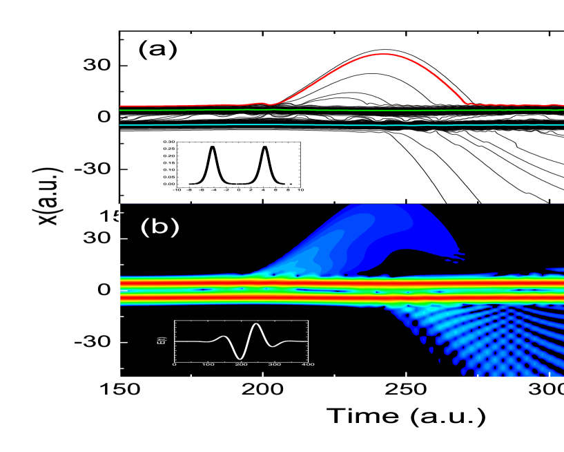
Figure 1: (Color online) (a) Time-volution of BTs; (b) time-volution of the electronic probability density and selected BTs BT(N) and BT(P).

In order to explore the generation mechanism of the minima structure in the H${}_{2}^{+}$ molecular HHG spectrum, we first calculate the BTs using Eq. (1). In the insert of Fig. 1 (a), we present the initial position of the the Bohmian particles that are sampled from the electronic density distribution of the ground state, which is calculated from the H${}_{2}^{+}$ molecular potential with $\alpha=0.4$ and $R=8.5$. In our calculation, the laser’s frequency is $\omega=0.057$, and the peak amplitude of the laser’s electric field is $E_{0}=0.1$, where the shape of the laser’s electric field is shown in the insert of Fig. 1(b). The Bohmian trajectories are shown in Fig, 1(a), where we may find that most of these trajectories are still located at around the two atomic nuclei and few trajectories are ionized after the laser pulse. In order to clearly distinguish the trajectories, we only present 400 trajectories in the Fig.1 (a). One may ask: can these un-ionized trajectories play a role in HHG? If the answer is yes, then how these bound BTs play roles in HHG? To answer these questions, we select two typical BTs which are initially located at -$R/2$ (BT(N)) and $R/2$ (BT(P)) respectively. The trajectory BT(N) is expressed in cyan curve, and BT(P) is expressed in green line in Fig. 1(a). We also present a recollision trajectory (the red curve) in Fig. 1(a). For the purpose of comparison, in Fig. 1(b), we present the time-evolution picture of electronic probability density distribution by solving TDSE. We can find that the time-dependent electronic probability density agrees well with the evolution of the BTs. Under the dominance of the laser’s electric field, the ionization mainly occurs at two moments ($t=200$ and $t=250$) which correspond to the peak positions of two half cycles of the laser electric field. Moreover, only for the ionization at about $t=200$, the ionized electron has chance to come back to the nucleus (red line in Fig. 1(a)).

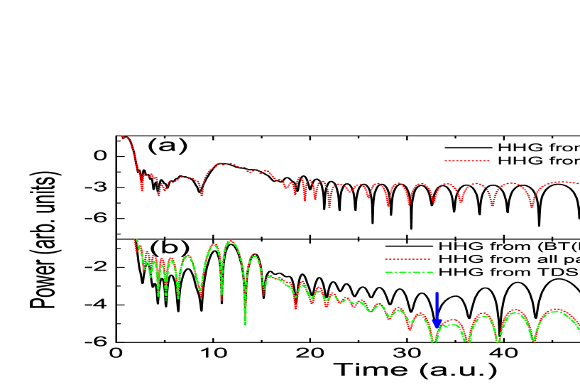
Figure 2: (Color online) Harmonic spectra from the diatomic molecule ion irradiated by the driving laser pulse, whose parameters are $E_{0}=0.1$ and $\omega=0.057$: (a) calculated from the BT(N) and BT(P); (b) calculated from the TDSE and coherent sum of two or all Bohmian particles.

Using the two selected trajectories BT(N) and BT(P), we calculate the corresponding harmonic spectra by Eq. (2). The results are presented in Fig. 2(a), where the solid black line is the harmonic spectrum calculated from the trajectory BT(N), and the dotted red line is the harmonic spectrum calculated from the trajectory BT(P). It can be seen from Fig. 2(a) that the two harmonic spectra have almost same intensities but different cutoffs. For the low order region of the harmonic spectra, their harmonic structures are similar with each other. As the harmonic order is larger than 30, the difference between these two harmonic spectra increases with the harmonic order. As we calculate the total harmonic spectrum by summing up the contributions of these two trajectories, a clear minimum at about 33rd harmonic order appears in the HHG spectrum caused by the interference between these two trajectories, as shown by a blue arrow in Fig. 2(b). This result qualitatively agrees with the results of the numerical calculation of TDSE and that by summing up the contributions of all the Bohmian trajectories ($N_{Tra}=50000$), as shown by the dash-dotted green line and dotted red line in Fig. 2(b), respectively.

In order to explain why only two BTs can simulate the structure of the whole HHG spectrum, we investigate the dynamic behaviors of the two corresponding Bohmian particles and their accelerations. The time evolution of BT(N) and BT(P) is presented in Fig. 3(a). From Fig. 3(a) we can see that two particles oscillate with time, whose oscillation amplitudes are proportional to the change of electric field amplitude. The behaviors of the two Bohmian particles are alike at the beginning of the laser pulse and exhibit the difference at the moment about $t=200$. At this moment, the trajectory BT(P) appears a fast oscillation whose frequency is about 10 $\omega$, while BT(N) moves smoothly. Furthermore, at about moment $t=250$, BT(P) moves smoothly while BT(N) oscillates. These oscillation mainly contributes to the low order harmonics in the HHG spectrum, and its generation mechanism has been explained by Wang et al 34 .

Because the radiation of a particle is proportional to the module square of its acceleration 35 , we present the corresponding acceleration of two particles in Fig. 3(b). It can be clearly seen from Fig. 3(b) that around the instant 200, only BT(P) oscillates with a non-negligible amplitude whose frequency is about 10 $\omega$. However, in the period of $t=230-300$, a fast oscillation with high amplitude appears for both Bohmian particles with almost the same amplitude. In order to clearly investigate the dynamic interference profile of the HHG, we focus on the accelerations of the two Bohmian particles in the period of $t=230-300$, as is shown in Fig. 3(c). From this figure one can see that the dipole accelerations of two particles have similar magnitude and oscillation frequency at every instant. However, their relative phase changes with time. In the regions ’A’, ’C’ and ’E’, their accelerations exhibit opposite phases, while in the regions ’B’ and ’D’ , their accelerations exhibit same phases. From the viewpoint of the quantum interference, we may predict that when the two oscillations have the same phases, the corresponding harmonic emission should be coherently enhanced; On the contrary, when the two oscillations have the opposite phases, the corresponding harmonic emission should be coherently reduced. To confirm our prediction, we perform the time-frequency analysis using wavelet transform for the Bohmian particles:

$${A_{\omega}}({t_{0}},\omega)=\int_{{t_{i}}}^{{t_{f}}}{{a_{k}}(t){w_{{t_{0}},\omega}}(t)dt}{\rm{,}}$$ (6)

where the wavelet kernel is ${w_{{t_{0}}{\rm{,}}\omega}}{\rm{=}}\sqrt{\omega}W{\rm{(}}\omega{\rm{(}}t{\rm{-}}{t_{0}}{\rm{))}}$, and Morlet wavelet36 ; 37 is used in this work.

It should be noticed that the dynamic emission profile of the harmonic can be clearly observed from the corresponding acceleration of the Bohmian particle. In Fig. 4(c), we present the time-frequency profile of the harmonic generated from the summation of BT(P) and BT(N). For the higher order harmonics, in the period of $t=230-300$, the interference pattern between these trajectories can be observed. Compared with time-dependent acceleration in Fig. 3(c), we find that, in time region of ’A’, ’C’ and ’E’, where the two particles are out of phase, the harmonic intensity is low. On the contrary, in the period of ’B’ and ’D’, the Bohmian particles’ accelerations are in phase, and hence the corresponding harmonic emission has higher intensity. Thus one can clearly observe the dynamic interference profile of molecular HHG through the analysis of BTs. The time frequency profiles of the harmonic generated from two Bohmian particles are shown in Fig. 4(a) and (b). In Fig. 4(d), we calculate the time-frequency profile from the dipole calculated from the TDSE. Comparing Fig. 4(d) with (c), we can find that, in the high energy part, this dynamic profile of HHG agrees well with the result by the coherent summation of the two Bohmian trajectories.

The reason why the main characteristics of the molecular harmonic spectrum can be generated by only two Bohmain trajectories which are located respectively at the two ions is that the two localized trajectories can receive and store the whole collision information coming from all of the other recolliding trajectories. The motion of Bohmian particle is not affected by classical force but also affected by the quantum force 21 . Therefore, using the information about the two BTs, we can detect the recolliding process.

III Conclusion

In conclusion, utilizing Bohmian trajectory scheme, the dynamic coherent process of the molecular high-order harmonic generation is investigated in this paper. Through analyzing the temporal characteristics of Bohmian trajectories, we found that the minima in the molecular HHG spectrum is attributed to the interference of the Bohmian trajectories located at the two centers of molecule. The Bohmian trajectory scheme can clearly reflect the dynamic process of harmonic interference, and can be taken as a detector to explore the dynamic process of complicated molecular system.

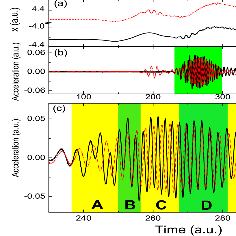
Figure 3: (Color online) Evolution of BTs BT(N) and BT(P): (a) time-dependent trajectories; (b) acceleration; (c) detailed acceleration.

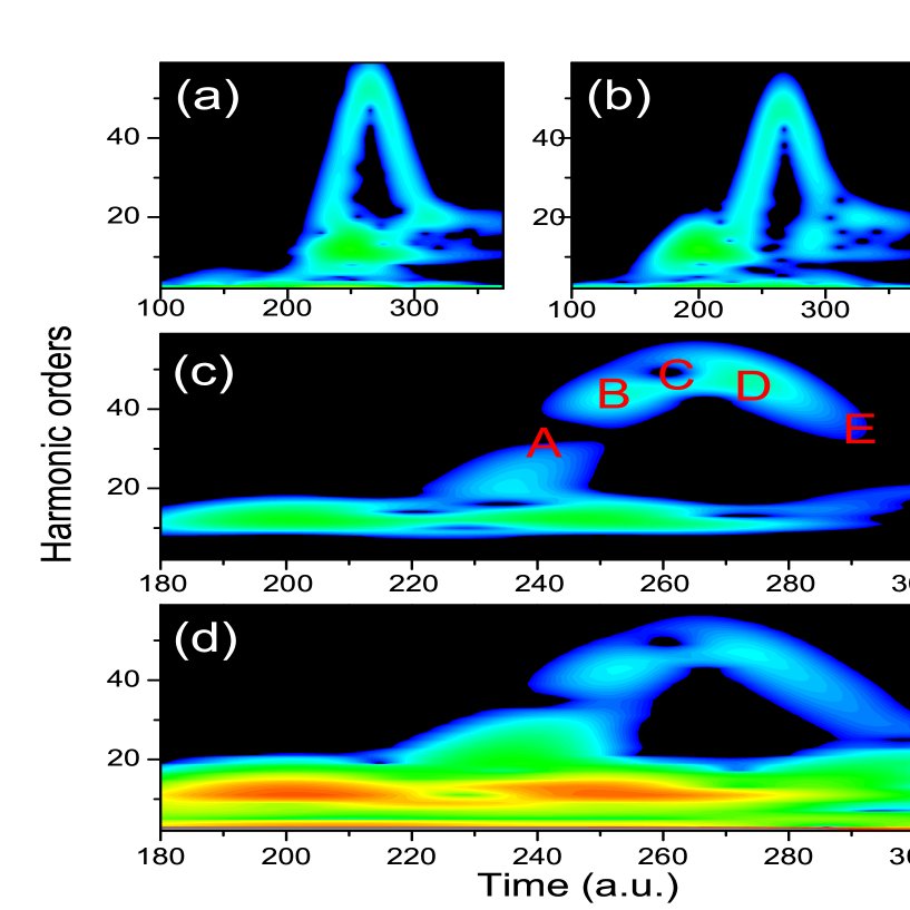
Figure 4: (Color online) Time-frequency behavior of harmonic emission calculated from: (a) BT(N); (b) BT(P); (c) coherent sum of BT(P) and BT(N); (d) TDSE.

- (1) A. McPherson, G. Gibson, H. Jara, U. Johann, T. S. Luk, I. A. McIntyre, K. Boyer and C. K. Rhodes, J. Opt. Soc. Am. B 4, 595 (1987).
- (2) M. Ferray, A. L’Huillier, F. Li, L. Lompre, G. Mainfray and C. Manus, J. Phys. B 21, L31(1998).
- (3) T. Popmintchev, M. C. Chen, D. Popmintchev, P. Arpin, S. Brown, S. Alisaukas, G. Andriukaitis, T. Balciunas, O. D. Mucke, A. Pugzlys, A. Baltusaka, B. Shim, S. E. Schrauch, A. Gaeta, L. Plajs, A. Becker, A. Jaron-Backer, M. M. Murnane and H. C. Kapteyn, Science 336,, 1287 (2012).
- (4) M. Lein, J. Phys. B 40, R135(2007).
- (5) P. B. Corkum, Phys. Rev. Lett., 71, 1994 (1993).
- (6) M. Lewenstein, P. Balcou, M. Y. Ivanov, A. L’Huillier and P. B. Corkum, Phys. Rev. A, 49, 2117(1994).
- (7) P. Salieres, A. Maquet, S. Haessler, J. Caillat and R. Taibeb, Rep. Prog. Phys., 75, 062401(2012).
- (8) E. Goulielmakis, M. Schultze, M. Hofstetter, V. S. Yakovlev, J. Gagnon, M. Uiberacker, A. L. Aquila, E. M. Gulikson, D. T. Attwood, R. Kienberger, F. Krausz, and U. Kleineberg, Science 302, 1614(2008).
- (9) F. Krausz, M. Ivanov, Rev. Mod. Phys. 81, 163 (2009).
- (10) J. Itatani, J. Levesue, D. Zeidler, H. Niikura, H. Pepin, J. C. Kieffer, P. B. Corkum, and D. M. Villeneuve, Nature (London), 432, 867(2004).
- (11) B. McFarland, J. Farrell, P. Bucksbaum and M. Guhr, Science 322, 1232 (2008).
- (12) S. Haessler, J. Caillat and P. Salieres, J. phys. B 44, 203001(2011).
- (13) W. Li, X. Zhou, R. Lock, S. Patchkovskii, A. Stolow, H. C. Kapteyn, and M. M. Murnane, Science 322, 1207 (2008).
- (14) O. Smimova, Y. Mairesse, S. Patchkovskii N. Dudovich, D. Villeneuve, P. Corkum, and M. Yu. Ivanov, Nature 460, 972 (2009).
- (15) H. J. Worner, J. B. Bertrand, D. V. Kartashov, P. B. Corkum, and D. M. Villeneuve, Nature 446, 604(2010).
- (16) M. Lein, N. Nay, M. R. Velotta, J. P. Marangos and P. L. Knight, Phys. Rev. Lett. 88, 183903 (2002).
- (17) N. Takemoto and A. Becker, J. Chem. Phys. 134, 074309 (2011).
- (18) X. Y. Lai, Q. Y. Cai and M. S. Zhan, New. J. Phys. 11, 113035 (2009).
- (19) A. S. Sanz, B. B. Augstein, J. Wu and C. Figueira de Morisson Faria (submitted for publication), pre-print arXiv:1205.5298
- (20) J. Wu, A. S. Sanz, B. B. Augstein and C. Figueira de Morisson Faria(submitted for publication), pre-print arXiv: 1301.1916
- (21) Y. Song, F. M. Guo, S. Y. Li, J. G. Chen, G. Chen and Y. J. Yang, Phys. Rev. A 86, 033424 (2012).
- (22) M. Lein, N. Hay, R. Velotta, J. P. Marangos and P. L. Knight, Phys. Rev. A, 66, 023805 (2002).
- (23) G. L. Kamta and A. D. Bandrauk, Phys. Rev. A 71, 053407 (2005).
- (24) T. Kanai, S. Minemoto, and H. Sakai, Nature 435, 470 (2005).
- (25) Y. Han and L. B. Madsen, J. Phys. B 43, 225601(2010).
- (26) A. Etches, M. B. Gaarde, and L. B. Madsen, Phys. Rev. A 84, 023418 (2001).
- (27) Y. Wu, J. T. Zhang, H. L. Ye, and Z. Z. Xu, Phys. Rev. A 83, 023417 (2011).
- (28) Y. C. Han and L. B. Madsen, Phys. Rev. A 87, 043404 (2013).
- (29) D. Bohm, Phys. Rev 85, 166 (1952).
- (30) D. Bohm, Phys. Rev 85, 180 (1952).
- (31) R. E. Wyatt 2005 Quantum Dynamics with Trajectories (NewYork: Springer).
- (32) Y. J. Yang, G. Chen, J. G. Chen and Q. R. Zhu, Chin. Phys. Lett. 21, 652 (2004).
- (33) Y. J. Yang, J. G. Chen, F. P. Chi and Q. R. Zhu, H. X. Zhang and J. Z. Sun, Chin. Phys. Lett. 24, 1537 (2007).
- (34) J. Wang, G. Chen, F. M. Guo, S. Y. Li, J. G. Chen and Y. J. Yang, Chin. Phys. B 22,033203(2013).
- (35) R. D. Cowan 1981 The Theory of Atomic Structure and Spectra (Univ of California Pr).
- (36) J. G. Chen, S. L. Zeng and Y. J. Yang, Phys. Rev. A. 82, 043401 (2010).
- (37) J. G. Chen, Y. J. Yang, S. L. Zeng and H. Q. Liang, Phys. Rev. A 83, 023401 (2011).