Exploring the Variable Sky with LINEAR. III. Classification of Periodic Light Curves
Abstract
We describe the construction of a highly reliable sample of 7,000 optically faint periodic variable stars with light curves obtained by the asteroid survey LINEAR across 10,000 deg2 of northern sky. The majority of these variables have not been cataloged yet. The sample flux limit is several magnitudes fainter than for most other wide-angle surveys; the photometric errors range from 0.03 mag at to 0.20 mag at . Light curves include on average 250 data points, collected over about a decade. Using SDSS-based photometric recalibration of the LINEAR data for about 25 million objects, we selected 200,000 most probable candidate variables with and visually confirmed and classified 7,000 periodic variables using phased light curves. The reliability and uniformity of visual classification across eight human classifiers was calibrated and tested using a catalog of variable stars from the SDSS Stripe 82 region, and verified using an unsupervised machine learning approach. The resulting sample of periodic LINEAR variables is dominated by 3,900 RR Lyræ stars and 2,700 eclipsing binary stars of all subtypes, and includes small fractions of relatively rare populations such as asymptotic giant branch stars and SX Phoenicis stars. We discuss the distribution of these mostly uncataloged variables in various diagrams constructed with optical-to-infrared SDSS, 2MASS and WISE photometry, and with LINEAR light curve features. We find that combination of light curve features and colors enables classification schemes much more powerful than when colors or light curves are each used separately. An interesting side result is a robust and precise quantitative description of a strong correlation between the light-curve period and color/spectral type for close and contact eclipsing binary stars ( Lyræ and W UMa): as the color-based spectral type varies from K4 to F5, the median period increases from 5.9 hours to 8.8 hours. These large samples of robustly classified variable stars will enable detailed statistical studies of the Galactic structure and physics of binary and other stars, and we make them publicly available.
1 Introduction
Variability is an important phenomenon in astrophysical studies of structure and evolution, both stellar, Galactic and extragalactic. Its importance will only increase with the advent of massive time domain surveys, such as Gaia (Eyer et al., 2012) and LSST (Ivezić et al., 2008a), where the expected number of identified variable stars will reach hundreds of millions – roughly the same as the number of all the stars detected by the Sloan Digital Sky Survey (SDSS; York et al., 2000). Such a large number of light curves can be fully analyzed only using automated machine learning methods (e.g., Debosscher et al., 2007; Dubath et al., 2011; Richards et al., 2011). Most such methods require reliable training samples; in addition to astrophysical motivation for improved understanding of the optical variability of faint sources, a goal of analysis presented here is to construct a large training sample of periodic variable stars that probes both a large sky area and faint magnitude range.
This paper is the third one in a series based on light curve data collected by the LINEAR (Lincoln Near-Earth Asteroid Research) asteroid survey in the period roughly from 1998 to 2009. In the first paper (hereafter Paper I, Sesar et al., 2011) we described the LINEAR survey and photometric recalibration based on SDSS stars acting as a dense grid of standard stars. In the overlapping 10,000 deg2 of sky between LINEAR and SDSS, photometric errors range from 0.03 mag for sources not limited by photon statistics to 0.20 mag at (here is the SDSS band magnitude). LINEAR data provide time domain information for the brightest 4 magnitudes of SDSS survey, with 250 unfiltered photometric observations per object on average (rising to 500 along the Ecliptic). The public access to the recalibrated LINEAR data, including over 5 billion photometric measurements for about 25 million objects (about three quarters are stars; 5 million objects have and photometric errors below about 0.1 mag) is provided through the SkyDOT Web site (https://astroweb.lanl.gov/lineardb/). Positional matches to SDSS and 2MASS (Skrutskie et al., 2006) catalog entries are also available for the entire sample. In this work we also provide positional matches to WISE catalog entries (Wright et al., 2012) for confirmed periodic variables.
In Paper I we compared LINEAR dataset to other prominent contemporary wide-area variability surveys in terms of depth and cadence. LINEAR extends the deepest similar wide-area variability survey, the Northern Sky Variability Survey (Woźniak et al., 2004), by 3 mag. This improvement in depth is significant; for example, it can be used to extend distance limit for Galactic structure studies based on RR Lyræ stars by a factor of 4 (to about 30 kpc; for details see the second paper in this series, hereafter Paper II Sesar et al., 2013). Thanks to the improved faint limit, the sample includes over a thousand quasars (for ; for detailed analysis see Ruan et al., 2012). The large sky area, with resulting increase in sample sizes, enables robust statistical studies of samples such as eclipsing binary stars, and searches for rare objects (e.g., field SX Phe stars, asymptotic giant branch stars). In addition to these specific programs, the depth improvement of 3 mag will help quantify the variation of the composition of the variable source population with depth. For example, Eyer & Blake (2005) determined that 83% of variable objects with are red giants, while in contrast Sesar et al. (2007) found that two thirds of variable objects with are RR Lyræ and quasars).
In order to make scientific use of the LINEAR dataset, the completeness and purity for samples of selected variable objects need to be understood and quantified. There are a number of automated methods for selecting variable objects and classifying their light curves proposed in the literature (e.g., Eyer & Blake, 2005; Debosscher et al., 2007; Dubath et al., 2011; Richards et al., 2011, and references therein). Measuring the performance of these methods on LINEAR dataset requires reliable training sample and full understanding of the photometric error distribution. It would be difficult to quantify the performance of these methods on LINEAR dataset because there are no reliable training samples, and the photometric error distribution is not fully understood yet. The LINEAR survey was not designed as a photometric survey, and more importantly, it accepted data obtained in non-photometric conditions. Although the LINEAR photometric error distribution obtained in Paper I is close to Gaussian, various tests show that of the order 1% of measurements can have anomalous errors (defined here as errors at least three times larger than reported errors) that are hard to recognize using available metadata (such as photometric zeropoint information and the photometric scatter for calibration stars). This problem could be explained by acquisition of data in non-photometric conditions (e.g. thin clouds or haze). A part of the problem may also be the fact that a large fraction of observations are obtained along the Ecliptic where contamination by blended main belt asteroids is not negligible.
Despite the fraction of measurements with anomalous errors as small as 1%, the resulting sample contamination can be substantial. According to Sesar et al. (2007), about 2% of objects with are variable at the 0.05 mag level (root-mean-square scatter, rms). Given that practical cutoff on rms is about 0.1 mag for the LINEAR dataset, and excluding quasars which are not numerous at magnitudes probed by LINEAR (fewer than 0.1% of objects in the LINEAR sample with are quasars), robustly detectable variability is expected for much less than 1% of the sample. Hence, even if only 1% of the LINEAR sample is spuriously selected as variable star candidates, the resulting false positives would dominate the sample.
LINEAR observing strategy produces repeat photometry data for stars on several timescales, ranging from 15-20 minute interval between images within a frameset, to a few days between repeat visits during one lunation, to the month-long timescale between lunar months, to the yearly. More details on the sampling pattern can be found in Paper I Appendix A.
In order to better understand the behavior of photometric errors in the LINEAR sample, and to ultimately enable deployment of automated methods for selecting variable objects and classifying their light curves, we have undertaken an extensive program of visual classification of about 200,000 light curves by eight human classifiers. Further details about visual classification and the construction of the resulting sample of about 7,000 robust periodic variables are described in §2. The distribution of periodic variables, dominated by roughly equal fractions of RR Lyræ stars and eclipsing binary stars, in various color-color and other diagrams is discussed in §3. We compare our results to existing variable star catalogs in §4, and to supervised and unsupervised machine learning classification methods in §5. Our main results are discussed and summarized in §6.
2 Visual Classification of LINEAR Light Curves
The main goal of our analysis is the selection of a large robust sample of periodic variable stars, with a high purity (i.e., low contamination) within adopted flux, amplitude and period limits. To improve the sample robustness and light curve classification, we undertook three successive selection and classification steps. After the initial sample selection, period estimation and construction of phased light curves, eight human classifiers extracted about 7,000 likely periodic variables from a starting set of about 200,000 candidate variables, and also obtained initial light curve classification. In the following two steps, a single expert refined selection and classification of the smaller sample of 7,000 likely periodic variables, first by repeating visual classification, and then further refined the candidate sample by adding the parameters measured from light curves and other information, such as multicolor photometry into the classification procedure. In this section we first describe the initial sample selection and period estimation, and then discuss the visual classification procedures in detail. A preliminary analysis of the resulting sample of robust periodic variables is presented in the next section.
2.1 Sample selection
We start by selecting candidate variables from the public LINEAR database111Available at https://astroweb.lanl.gov/lineardb/ using the following criteria:
-
•
Brightness limit: , where is the median value of the white-light LINEAR magnitude222The faint magnitude limit adopted in Paper II is 0.5 mag fainter than adopted here because ab type RR Lyræ discussed in Paper II are easier to recognize than other types of variable object discussed here..
-
•
Likely variability: , where per degree of freedom is computed using the unweighted mean magnitude and photometric errors reported in the database.
-
•
Variability amplitude: mag, where is the rms scatter (standard deviation) of recalibrated LINEAR magnitudes.
The majority of about 200,000 selected objects are found in the region bounded by and (corresponding to the North Galactic Cap scanned by SDSS). Additional 8,000 objects are found in the SDSS Stripe 82 region ( and ). The selected objects contain both true variable objects and spurious candidates. We limit our classification to objects exhibiting mono-periodic variability (light curves that satisfy , where is the period and is positive; assuming no noise), and use phased light curves for visual inspection. Phased light curves are constructed by plotting as function of phase
| (1) |
where the function int() returns the integer part of . The likely periods were determined as described next.
2.2 Period finding methods
For each selected object, the three most likely periods were found using using an implementation of the Supersmoother algorithm (Friedman, 1984; Reimann, 1994). This non-parametric method smooths the light curve using a variable smoothing length and uses cross-validation method to pick a best-fit period with the smallest phased light curve dispersion. The Supersmoother algorithm was extensively used by the MACHO survey and should be robust for a large variety of variable stars because it makes no explicit assumptions about the shape of the light curve.
During the classification it soon became apparent that the Supersmoother algorithm often had problems with finding the correct period; for eclipsing binaries in particular a large fraction of best-fit periods were twice as short as the true period (we will return to this discussion in §2.3.7). For this reason, we also included two additional algorithms for estimating periods: the Lomb-Scargle (LS) and Generalized Lomb-Scargle (GLS) parametric methods (Lomb, 1976; Scargle, 1982; Zechmeister & Kürster, 2009). We used the code implemented in Gaia’s Coordination Unit 7 pipeline (Eyer et al., 2013).
The LS method essentially fits a single sine wave to the light curve, and is capable of using heteroscedastic errors. It assumes that the true light curve mean is equal to the mean of sampled data points. In practice, the data often do not sample all the phases equally, the dataset may be small, or it may not extend over the whole duration of a cycle: the resulting error in the estimated light curve mean can cause problems such as aliasing. A simple remedy implemented in the GLS algorithm is to add a constant offset term to the single sinusoid model (Zechmeister & Kürster, 2009).
We note that when the light curve shape significantly differs from a single sinusoid, the LS and GLS methods may easily fail. Possible remedies in such cases are to fit pre-defined light curve templates (e.g., Sesar et al., 2010), or to use multiple harmonics in the Fourier expansion, which we have not considered here (e.g. Figures 4 and 5).
2.3 Visual classification methodology
Visual classification was performed on a per-object basis. There were three classification/validation runs; the first run pruned the list of candidates by more than a factor of 20, and the subsequent two runs further improved the sample purity and light curve classification precision. In the first run, 200,000 variable star candidates were divided roughly equally among eight human classifiers, using right ascension boundaries, and each classifier processed approximately 30,000 light curves. Overlaps of 2,500 light curves between the samples of the “adjacent” classifiers were used to verify classification consistency (which was assessed as described in §2.3.2 and 2.3.4).
2.3.1 Initial visual classification
The initial visual classification was performed using the user interface shown in Figure 1. The automated classification tool displayed three phased light curves, folded with the periods found by the Supersmoother period finding algorithm, as well as five templates of folded (phased) light curves spanning predicted classes of variable objects. Classifiers answered three questions with fixed possible answers.
The first question was whether the displayed phased light curves have “reasonably small” dispersion around some imaginary smooth shape, following the Phase Dispersion Minimization idea of Stellingwerf (1978). There were four possible answers to this question (coded by numerical values in parentheses): “definitely no” (0), “probably no, but not sure” (1), “probably yes, but not sure” (2), “definitely yes” (3). Unless the answer to the first question is “definitely no”, classifier proceeds to the second question related to the light curve shape. Possible answers are: “does not look like any template” (0), “RR Lyr ab” (1), “RR Lyr c” (2), “single minimum on top of a flat light curve” (3), “two minima on top of a flat light curve with some flat part” (4), “two minima without the flat light curve part” (5). The third question asks the user to choose which of the three folded light curves of the given object shows the smallest dispersion (the intention was to determine which of the three periods is the best). In addition, there was an option to add comments if necessary (e.g., about period aliasing, or any problems with the data), or to go back and repeat the classification for the object if an error was made. By design, only the light curve shape was used in this first classification stage.
After a brief training period, it takes about 5 seconds on average to answer all three questions, for a throughput of 700 objects per hour (about a week worth of full-time work per classifier, or about 2 Full-Time-Equivalent person months for the whole effort, assumming an unrealistic efficiency of 100%).
2.3.2 Tests of the initial classification uniformity and repeatability
In order to assess the uniformity and repeatability of the visual classification, a subsample of 8,044 light curves was classified by all eight classifiers. These objects were selected from the SDSS Stripe 82 region so that a comparison with an SDSS-based variable object catalog can also be performed (described further below).
For each light curve, we averaged the eight answers to question 1 (ranging from 0 for “definitely not variable” to 3 for “definitely variable”) to obtain its “grade”. We also computed its standard deviation among the eight classifiers, , to quantify dispersion in classification grades. Based on the morphology of the distribution, we divided the sample into four subsamples using , as summarized in Table 1. The 317 light curves with have the smallest : that is, most classifiers agree that these 3.9% objects are “definitely variable”. The classification robustness of other light curves is lower, as seen from the increased dispersion among the classifiers.
After sorting light curves by , two coauthors have re-inspected all 438 light curves with (classes 1-3), as well as 1000 light curves from class 0 with highest values. No spurious classifications were found in class 3. Objects in class 2 seem definitely variable, but many appear to have incorrect periods. Class 1 is similar to class 2, except for a larger fraction of unconvicing periodic cases. Therefore, there are between 317 and 438 definite periodic variables in this sample, depending on how conservative a selection cut is adopted, implying an upper limit for the sample contamination of 28%. Our main conclusion is that human classifiers are mutually consistent when their answer to the first classification question is 2 or 3, that is, when they are highly confident about detected variability.
2.3.3 Robust Selection
The LINEAR light curve database contains two values of : the standard value and the so-called robust , , determined by excluding both brightest and faintest 10% of points from the computation (note that despite its name, the measured does not follow the statistical distribution expected for Gaussian photometric errors). The robust might be efficient at minimizing the impact of photometric outliers, but at the same time it may decrease the sample completeness for light curves where variability is not always present (e.g., bursts and Algol-like light curves).
We have investigated whether can be used to significantly prune the initial sample without a large decrease in the final sample completenesss (that is, whether -based selection could be used instead of visual pruning of the candidate sample). If selection is adopted (instead of ), the size of the initial sample decreases from 200,000 to 80,000. Of all the light curves with (classes 2 and 3 above, see Table 1), 86% have . Therefore, the initial sample could be made smaller by a factor of 2.5, while losing 10-20% of true variables. This tradeoff reflects both the properties of faint variable stars and the behavior of LINEAR photometry.
About 14% of light curves with (robust variables, as suggested by visual classification) have (no strong evidence for variability). We have re-inspected these puzzling cases and found that they all are indeed real variables. In other words, visual classification is correct but is too conservative a cut – these objects mostly have small amplitudes, short-duration peaks, or are faint (and thus photometric errors are large). Therefore, it should be possible to extract additional variable stars from the LINEAR database because our initial sample of 200,000 candidates had to satisfy .
We have also re-inspected a random sample of light curves with and , that is, light curves that show significant variability according to but were not visually classified as periodic variables. About a half of these light curves show significant variability which appears aperiodic. A subset of a few hundred light curves with periods exceeding 1000 days and seem consistent with being semi-regular variable asymptotic giant branch stars. Therefore, their rejection from the periodic light curve sample during visual classification is justified.
In summary, parameter cannot be used to replace the visual classification step by automated selection without a significant drop in the sample completeness.
2.3.4 Comparison to the variable star sample from the SDSS Stripe 82
SDSS has obtained multiple observations (about 50 on average) in the large
so-called Stripe 82 region. These data were used to select 67,507 candidate variable point
sources333Light curves are publicly available from
http://www.astro.washington.edu/users/ivezic/sdss/catalogs/S82variables.html
(for details see Ivezić et al. 2007a; Sesar et al. 2007; and references therein).
There are many more candidate variables per unit sky area in the SDSS Stripe 82
catalog than in LINEAR sample because the former is much deeper ( vs.
) and has a more inclusive cutoff for variability rms (0.05 vs. 0.1 mag). We
have used this SDSS catalog to assess the reliability and completeness of
candidate variables visually selected from LINEAR database.
Out of 8,044 LINEAR objects found the Stripe 82 region, 543 have positional matches within 2 arcsec to candidate SDSS variables that show periodic behavior. Of those, 301 have , that is, 83% of 363 robust LINEAR variables are confirmed by SDSS data. Therefore, there are 62 robust LINEAR variables that are not in SDSS variable sample, representing an 11% addition to the SDSS sample. These 62 LINEAR variables are dominated by detached eclipsing binaries with most SDSS observations falling along the flat part of light curve. An example is shown in Figure 2. Therefore, the implied purity of LINEAR variables must be higher than 83%, and is consistent with 100% (that is, we did not find a single questionable case among these 62 variables). Figure 2 also demonstrates synergy between the SDSS and LINEAR datasets: while LINEAR provides much better time-resolved photometry for studying variable objects, SDSS provides very informative 5-band photometry.
About 45% of SDSS variables which are sufficiently bright to be in LINEAR sample are not selected from LINEAR database using criteria listed in §2.1 and based on visual classification. About one third of those could be recovered by relaxing the limit. The remaining two thirds (30% of all SDSS variables) typically have sparse LINEAR data and/or small variability amplitudes, and thus were justifiably rejected in visual classification. Therefore, relative to the SDSS subsample limited to a similar depth, the completeness of the LINEAR sample is in the range 55-70%, depending on the adopted cut (most of the LINEAR incompleteness is due to larger adopted minimum rms variability, 0.1 mag vs. 0.05 mag).
Finally, out of 301 stars that are recognized as periodic variables by both SDSS and LINEAR, 184 have LINEAR and SDSS periods that agree within 2%. Additional 57 objects have periods aliased by a factor of 2 in either SDSS or LINEAR (for one third of those, the SDSS periods are larger); they include a large fraction of eclipsing binary systems with similar depths of primary and secondary minima.
2.3.5 Iterative improvements to visual classification
The first classification step, which pruned the initial list of 200,000 candidate variables by more than a factor of 20, was performed by eight different classifiers which must have introduced some non-uniformity in the resulting classification. In addition, the resulting sample contamination could be as high as 17%, as discussed in §2.3.2 and §2.3.4. To improve sample purity and classification uniformity, all the objects tagged as plausibly variable in the first round were re-examined in the second round by the first author. Only a few percent of objects had their classification changed as a result of this re-examination. Generally, no significant variations among the eight subsamples were noticed, in agreement with the conclusions from the previous sections.
When the available source attributes (period, amplitude, and skewness of light curves, and optical and infrared colors) were analyzed for the sample obtained in the second classification round, it became apparent that different types of variable stars cluster in different regions of the multi-dimensional attribute space. Using selection boundaries based on color, period, amplitude and light curve skewness listed in Table 2, and discussed in more detail in the next subsection (§2.3.6), an additional sample of about 750 objects was selected from the initial candidate sample of 200,000 objects. That is, about 10% more potential variables than extracted in the first classification round were selected for further inspection.
Visual inspection of these 750 candidates (by the first author) in the third classification round revealed that only about 10% represented convincing cases of periodic variability. They were added to the initial list to produce the final sample of 7,194 visually selected and classified periodic variables. Among those, 6,876 light curves (96%) have been assigned a definite type, while the remainder are classified as “Other”. The latter group contains objects which are variable, but not periodically and objects for which the exact variability type could not be reliably determined.
The six main light curve types are listed in Table 2, and a few supplemental ones in Table 3, and discussed in more detail in the next Section. Hereafter, we refer to this entire sample as “visually confirmed sample of periodic LINEAR variables”, or simply “PLV” sample. The resulting catalog is made publicly available444Available from http://www.astro.washington.edu/users/ivezic/r_datadepot.html.
Table 3 quantitatively summarizes the results of visual classification. The first column “translates” our numerical codes used during visual classification to the adopted variability types. We hypothesize that the class “3” (“a single minimum on top of a flat light curve) mostly consists of EA type binaries (Algols) for which our data did not show a discernible secondary minimum (i.e. either too shallow to be detected, or too similar in depth to the primary minimum, recall §2.3). For that class of objects correct periods could be twice longer than listed in the catalog. The light curves classified as “5” include two types of eclipsing binaries: EB (or Lyræ) and EW (W Ursae Majoris), which are grouped together because they are hard to distinguish using only LINEAR light curves. Motivated by the distribution in period-color and period-amplitude diagrams, we introduced two additional classes: class “6” (containing SX Phoenicis and Scuti candidates) and class “7” (long-period variables defined here as variables with periods longer than 50 days, and as semi-regular variables). Further explanations regarding introduction of these two additional classes can be found in §3.4 and §3.5.
2.3.6 Simple automated classification with the aid of other attributes
The clustering of objects in different regions of the multi-dimensional attribute space offers an opportunity to develop automated classification methods. Here we define selection boundaries using simple, rectangular cuts in the four-dimensional attribute space (period, amplitude, skewness, color). Alternative approaches based on machine learning algorithms are discussed in Section §4. The adopted boundaries are listed in Table 2. We limit quantitative analysis of the performance of this classification scheme to ab and c type RR Lyræ, EB/EW eclipsing binaries and SX Phoenicis/ Scuti candidates. We do not include classes whose size does not exceed 1% of the full sample, nor Algols (EA eclipsing binaries) and objects classified as “Other”. We do not include Algols because their distribution does not have well-defined boundaries (not too surprising since in the case of detached binaries we could easily have an ensemble of paired objects with presumably few common physical characteristics). An analogous diversity is expected among long-period variables which include both Miras and semi-regular variables, and possibly other classes of variable stars. Indeed, even the definition of Mira stars suffers from quantitative ambiguity (“red long-period variables with visual amplitudes exceeding 2.5 mag”), although it has been shown that they are actually fundamental mode pulsators — a physical characteristic that differentiates them from other long period variables (e.g. Wood & Sebo, 1996; Soszyński et al., 2009; Spano et al., 2011).
In order to maintain analysis uniformity, we use best-fit periods found by the classic Lomb-Scargle method. Objects with unreliably measured SDSS colors, and Lomb-Scargle periods close to one day and half a day (0.05 tolerance in log) were excluded from the analysis. The performance of this supervised classification is statistically compared to our visual classification results in Figure 3. We have visually re-examined all 3,270 light curves with differing visual and automated classifications.
The automated method selected 74% of PLV objects from the four analyzed types. This result does not imply a 26% contamination in the PLV catalog but rather an incompleteness of the automated selection method; the majority of missing objects had unreliable SDSS colors, were rejected by the period cut, or had at least one of the attributes outside the allowed interval. This selection fraction varies little among the four types (see the bottom row in Figure 3).
The automated selection method selected additional 835 objects that are not included in the PLV catalog (a 12% addition, varying from 4% for c type RR Lyræ to 23% for EB/EW). Of those 835 objects, 246 correspond to ab type RR Lyræ; the majority are located very close to the red cutoff for the color. Approximately 15% of these 246 objects have light curves hinting at ab type RR Lyræ, but not of sufficient quality to enable reliable visual confirmation. Therefore, at most about 40 ab type RR Lyræ included in the initial sample of 200,000 candidates are missing from the PLV catalog (1.4% effect). In case of c type RR Lyræ, 44 objects not in PLV are uniformly distributed throughout the selection volume. About 30% of these objects have light curves that might be classified as c type RR Lyræ, though not reliably. Similar behavior is displayed in EB/EW case, with only about 10% of 545 objects not in PLV potentially classifiable as reliably periodic. Therefore, the PLV catalog is only slightly incomplete relative to the initial sample of 200,000 candidates (by about 1-2% at most).
The automated classification is correct for a high fraction of PLV objects: 97% for ab type RR Lyræ, 78% for c type RR Lyræ, 87% for EB/EW, and 100% for SX Phe/ Sct. In summary, this analysis provides further support that the PLV catalog is highly complete relative to the initial sample of 200,000 candidate variables, has exceedingly low contamination, and a high rate of correct light curve classification.
2.3.7 Comparison of period finding methods
As we already indicated earlier, period finding algorithms often had problems with choosing the correct period. For example, for eclipsing binaries a large fraction of best-fit periods were twice as short as the true period. In this particular case, such behavior is easy to understand: primary and secondary minima are often of similar depth and are therefore often misidentified as the same feature in the phased light curve. This error, however, is not seen consistently: not all of the objects with similar depths of minima have periods that are too short by a factor of two.
Given the final sample of 6,876 reliably classified light curves, we tested period finding methods for each of the six main light curve types separately. Our results are summarized in Figure 4. We left the “single minima on top of a flat light curve” class out of the analysis, as the sample is small (20 objects) and the correct period for those objects could not be identified with certainty. We speculate that those objects could correspond to eclipsing binaries of EA (Algol) type with similar depths of minima, but with periods that are too short by a factor of two. Another explanation would be that secondary minima for these objects are too shallow to be detected in LINEAR data.
Our results show that the Lomb-Scargle and generalized Lomb-Scargle methods typically outperform the Supersmoother algorithm for all variability types. For c type RR Lyræ, long-period variables, and SX Phe/ Sct type light curves, Supersmoother has a much larger fraction of overestimated periods (typically by a factor of two, but sometimes more) than the other two methods. In addition, when the period is approximately correct, the uncertainty is typically larger for Supersmoother values (that is, the width of the central peak in histograms shown in Figure 4 is larger).
The performance of the period finding algorithms for eclipsing binaries is rather different: while the Lomb-Scargle and generalized Lomb-Scargle methods produce narrower histogram peaks than Supersmoother, their periods are consistently (at 90% level) too short by a factor of two! After an overall correction of periods for eclipsing binaries by this factor, the Lomb-Scargle and generalized Lomb-Scargle methods display better performance than Supersmoother.
The reason for this consistent bias in period estimation by the Lomb-Scargle and generalized Lomb-Scargle methods is their fundamental assumption that the shape of the underlying light curve can be described by a single sinusoid. A remedy is to fit a Fourier series with many terms (but more computationally expensive). As illustrated in Figure 5, a Fourier series model with six terms correctly recognizes two minima in the light curve of an eclipsing binary star. For additional discussion, please see Hoffman et al. (2009) and Wyrzykowski et al. (2003).
During the visual inspection it was relatively easy, albeit time consuming, to apply this correction factor to the periods. In a fully automated classification scheme that has only single band light curves and no color information this might be more difficult since values of period, amplitude and skewness are in large part similar for c type RR Lyræ and EB and EW binaries. Addition of appropriate color information (e.g. ) easily breaks this degeneracy (see §3.1 and §3.2). Ultimately, the performance of period finding algorithms based on a single sinusoid can be significantly improved by including more Fourier terms.
3 Analysis of Periodic LINEAR Variables
The remainder of our analysis is performed using the public version of the PLV catalog. We show in this section that the distribution of selected periodic variables displays distinctive features in the multi-dimensional attribute space spanned by the light-curve parameters (period, amplitude, shape) and optical/infrared colors. This behavior enables robust and efficient classification of objects into various classes of variable population. These features are not seen for the full sample of 200,000 candidate variable objects, and thus strongly suggest that visual classification successfully extracted true variables.
We first discuss the distribution of classified variables in diagrams constructed with the three light curve parameters, and then investigate the correlation of light curve parameters with optical and infrared colors. We quantify a strong correlation between the period and optical color for contact eclipsing binaries, provide evidence that the sample contains a large number, compared to the known objects, of likely Population II field SX Phe stars, and demonstrate that the infrared colors from the WISE survey provide further support that long-period variables are correctly classified.
3.1 Analysis of Light Curve Properties
The light-curve amplitude is estimated non-parametrically from the cumulative magnitude distribution as the range between the 5% and 95% points. The light-curve skewness is computed as described in Sesar et al. (2007). Therefore, light curves are quantitatively described using three parameters: period, amplitude and skewness. This choice is of course not unique. For example, in addition to, or instead of, amplitude, other estimators of the width of the observed magnitude distribution could be used, such as standard deviation (which is not robust to outliers) and the inter-quartile range (which, depending on the sampling, might not be sensitive to single minima in otherwise flat light curves). Similarly, the light-curve shape could be further quantified using higher moments (such as kurtosis, but they quickly become very noisy), Fourier coefficients (which help greatly to classify eclipsing binary subtypes (Pojmański, 2002), or RR Lyrae subtypes (Soszyński et al., 2011)), or even non-parametrically using the principal component analysis (e.g. Deb & Singh, 2009). In this preliminary analysis, we find that even our simple approach based on period, amplitude and skewness provides informative description of the light curve behavior. Nevertheless, exploring these other options would be a worthwhile analysis to undertake.
The distribution of variables in the period–amplitude–skewness space is illustrated separately for each of the six main variability classes in Figure 6. The period distribution of the PLV sample is multi-modal, as further quantified in Figure 7. Even the period alone enables remarkable, although not perfect, classification of periodic variables: SX Phe/ Sct candidates clearly stand out ( day), and ab type and c type RR Lyræ are fairly well separated by 0.4 days. Nevertheless, eclipsing binaries overlap with the period range of RR Lyræ stars (especially EW/EB type eclipsing binaries and c type RR Lyræ). In addition, the light-curve amplitude distributions are similar for c type RR Lyræ and EB/EW eclipsing binaries. This degeneracy can be readily lifted using the light curve skewness (and object color, see below). Indeed, all six classes can be readily defined when all three light-curve parameters are considered (e.g. EB/EW class has much larger skewness than c type RR Lyræ; compare the symbol color in the top right and bottom left panels in Figure 6). In other words, the visual classification of light curves in essence reflects the distribution of these three parameters (and also of the light curve smoothness). We analyze the performance of automated classification methods based on this behavior in §4.
It is possible to further separate ab type RR Lyræ into Oosterhoff type I and Oosterhoff type II stars (Sesar et al., 2010), as shown in the top right inset in the “RRAB” panel of Figure 6 (note also the strong correlation between the amplitude, skewness and period for ab RR Lyræ). Average periods of Oosterhoff type I and type II ab RR Lyræ for the PLV sample are days and days. This result is in good agreement with Oosterhoff’s conclusion that period of RR Lyræ ab in Oosterhoff type I clusters is 0.1 day shorter than that of those in Oosterhoff type II clusters (Oosterhoff, 1944). For a more detailed analysis of the Oosterhoff’s dichotomy for field RR Lyræ stars based on this sample, see Sesar et al. (2013).
3.2 Correlations between Colors and Light Curve Properties
The addition of the color information to light-curve parameters significantly improves the separation of visually defined classes and ultimately enables better performance of automated classification methods. For a detailed discussion of the distribution of stars in various color-color diagrams constructed with SDSS and 2MASS photometry, see Covey et al. (2007), and references therein. The most useful SDSS-2MASS colors are , (or ), and , which are sensitive to various combinations of effective temperature, metallicity, and surface gravity. Therefore, the minimal useful dimensionality (the number of measured attributes that are independent for at least some subsamples) of this dataset is at least five (the three light curve attributes and at least two color attributes).
We emphasize that both SDSS and 2MASS photometry are single-epoch measurements obtained at random light curve phases. Therefore, while the observed color range tracks the intrinsic color range of a given population, distribution of objects within that range is affected by the color light curve shape (e.g. ab type RR Lyræ stars spend more time close to minimum than to maximum light; since RR Lyræ are redder when fainter, their instantaneous color distribution is skewed redwards compared to their mean color distribution).
Figure 8 demonstrates that the addition of just one color to the period, here the SDSS color which is a good measure of the effective temperature (Ivezić et al., 2008b), helps to clearly separate c type RR Lyræ from EB/EW binaries. A more detailed illustration of the correlations between the color and light curve properties is shown in Figure 9. Note in particular how EA and EB/EW are well separated in this diagram. The EB/EW subsample displays a good correlation between the period and color, discussed in more detail in §3.3.
3.2.1 The vs. diagram
In addition to the three-dimensional color–period–amplitude projection of the full multi-dimensional attribute space discussed above, the three-dimensional projection spanned by the SDSS and colors and light curve skewness is also rich in content. The vs. diagram is one of the most informative SDSS color-color diagrams; it clearly distinguishes quasars from stars, main sequence stars from binary stars and white dwarfs, and it contains information about effective temperature and even metallicity for blue main sequence stars (Smolčić et al., 2004; Ivezić et al., 2007a, 2008b).
The distribution of variables in the vs. vs. skewness space is shown separately for each of the six main variability classes in Figure 10. As known from previous work based on SDSS data, RR Lyræ color distribution is localized to the region populated by spectral types A and early F (Sesar et al., 2010, and references therein). Only about 1-2% of light curves classified as RR Lyræ fall outside the expected small color regions discernible in Figure 10.
Based on the vs. color-color diagram and the skewness distributions, we identified approximately 25% suspected misclassifications between c type RR Lyræ and EB/EW eclipsing binaries (from the first classification round) and visually re-inspected their light curves. We found that approximately 80% of those were indeed likely misclassifications and their type was subsequently revised. The cross-contamination of these two subsamples is easy to understand; a light curve of an eclipsing binary with similar depths of minima can easily be misidentified as a nearly symmetric (sinusoidal) c type RR Lyræ light curve. This ambiguity is particularly problematic in case of faint objects, or objects with sparsely sampled light curves. We note that the color distribution of c type RR Lyræ has a well defined red edge – it is thus easy to prevent the contamination of EB/EW subsample by c type RR Lyræ but the converse is not true because EB/EW stars can have colors as blue as RR Lyræ colors.
We have also explored a few other three-dimensional projections of the seven-dimensional attribute space (there are 35 possible independent attribute combinations) and did not find diagrams as revealing as the color vs. period vs. amplitude diagram and the vs. vs. skewness diagram. A noteworthy color is the 2MASS color which is capable of separating main sequence stars from quasars and late-type giants (including the long-period asymptotic giant branch stars); for main sequence stars the 2MASS color and the SDSS color are highly correlated (both are by and large driven by the effective temperature), while for those other populations the measured color is redder than the color of main sequence stars of the same color (for more details, see Covey et al., 2007).
3.3 Period-color correlation for contact eclipsing binaries
The distribution of EB ( Lyræ) and EW (W Ursae Majoris) eclipsing binary stars is remarkably well outlined in the period vs. color diagram (see the bottom left panel in Figure 9, and a zoomed-in version in Figure 11). Since the sample selection is primarily driven by the light-curve shapes, and substantial selection effects in the color and period in the relevant ranges are not expected, this strong correlation is likely of astrophysical origin. A similar result was reported for a much smaller sample of contact binary systems by Eggen (1967) (see also Rucinski & Duerbeck, 1997, and references therein). The range of observed colors correspond to spectral types from F5 () to K4 () (see Table 3 in Covey et al., 2007). Rucinski & Duerbeck (1997) used Hipparcos distance estimates for 40 W UMa stars to derive a relationship between the absolute band magnitude, period and color. According to their results, our sample includes stars with .
We compute the median in bins of the color for stars with and , and fit a parabola to the resulting points,
| (2) |
Due to the large sample size, the random errors for the fitted data points are sufficiently small to rule out a linear relationship. This best-fit relation implies that the median period for EB/EW eclipsing binaries increases from 5.9 hours to 8.8 hours as the color-based spectral type varies from K4 to F5. An alternative form based on the Johnson color, derived using using transformations between the SDSS and Johnson systems from Ivezić et al. (2007b), is
| (3) |
and valid in the range . This relation agrees well with a similar relation obtained by Rucinski (1997) for 400 W UMa stars observed by the OGLE project in Baade’s window (note that we fit the median relation and Rucinski obtained the short-period limit as a function of color; the two sequences are offset by about 0.1-0.15 mag at a given period).
These findings are related to the fact that the period distribution for contact binary star systems appears to have a well-defined lower limit at 0.22 days (Rucinski, 1992). More recent data show that this limit may be a bit smaller (0.20 days, see Dimitrov & Kjurkchieva 2010; Davenport et al. 2013), but the existance of a well-defined boundary is not disputed. Indeed, the falloff of the distribution at small periods for M dwarf systems (see Figure 6 in Becker et al. 2011) is very similar to the falloff for EB/EW systems in our Figure 6. If we extrapolate our best-fit to corresponding to the spectral type M0, we obtain a period of 0.22 days in good agreement with other studies.
In Figure 12 we show several examples of these short period binaries. Several objects have periods below 0.2 days and test the value of the aforementioned period boundary.
3.4 Candidate SX Phe stars
The PLV sample presented here includes a class of 112 blue stars (, bluer than thick disk and halo turn-off stars and corresponding to using transformations between the SDSS and Johnson systems from Ivezić et al. 2007b), with very short periods (1–2.5 hours), and with asymmetric light curves (see bottom right panel in Figures 6 and 9). These stars can be identified as a mixture of Scuti and SX Phoenicis stars (e.g. see Figure 8 in Eyer & Mowlavi, 2007). Both types of stars are usually considered as variable counterparts of blue straggler stars (main sequence stars in open or globular clusters that appear younger than they should be given the cluster age), with Sct subsample belonging to Population I disk stars and SX Phe subsample to Population II halo stars (see e.g. Jeon et al., 2004).
In a recent study based on the largest catalog of SX Phe stars assembled to date (about 250 stars identified in globular clusters), Cohen & Sarajedini (2012) demonstrate that this population appears to occupy a narrow region at the bottom of the instability strip with , and are all likely radial mode pulsators. Given the apparent magnitude limits of our sample, the implied distances span the range 2–10 kpc, that is, many disk scale heights away, and thus SX Phe probably dominate because they are Population II (halo) objects. We note that the color distribution of our sample extends to bluer colors than the range displayed by the Cohen & Sarajedini (2012) sample (their range is approximately , corresponding to ; about 20% of our candidates have ).
A much higher fraction of SX Phe stars than Sct stars in this sample is supported by SDSS spectra that are available for 34 stars in the candidate sample. All the spectra appear very uniform and characteristic for A stars; an example is shown in Figure 13. Using the default SDSS metallicity and radial velocity estimates (see Figure 14), we find that the sample is dominated by stars with [Fe/H], low metallicities characteristic of halo stars, with a large velocity dispersion (134 km/s) that is also consistent with presumed halo population (for a review of recent observational constraints on the differences between the metallicity and kinematics distributions of disk and halo stars, see e.g. Ivezić, Beers & Jurić, 2012).
Assuming that our conclusion about the sample being dominated by halo stars is correct, these 112 candidates likely represent a major addition to the total number of known SX Phe stars (according to Cohen & Sarajedini, 2012, fewer than 300 SX Phe stars are known). Our sample would also increase the number of known field SX Phe stars by as much as a factor of six (according to Rodríguez et al., 2001, there are only 17 known field SX Phoenicis known). This large increase in the sample size of field SX Phe stars is due to the fact that the LINEAR dataset is among the first ones to explore sufficiently faint flux levels, over a large sky area, and with appropriate cadence. We are currently undertaking photometric and spectroscopic followup efforts to better characterize this sample.
3.5 Candidate AGB stars and WISE color distribution
The PLV sample includes 77 light curves classified as “long-period variables”, defined here as variables with periods longer than 50 days, and as semi-regular variables. These stars are expected to be dominated by asymptotic giant branch (AGB) stars which often display infrared excess emission due to their dusty envelopes (see e.g. Ivezić & Elitzur, 1995, and references therein). The correctness of their classification can thus be tested by inspecting their infrared colors.
The best available infrared sky survey was obtained by the recent Wide-field Infrared Survey Explorer (WISE, launched in 2010); its all-sky catalog includes about 560 million objects (Wright et al., 2012). WISE mapped the sky at 3.4, 4.6, 12, and 22 m with 5- point source sensitivities better than 0.08, 0.11, 1 and 6 mJy (corresponding to Vega-based magnitudes 16.5, 15.5, 11.2 and 7.9, respectively) in unconfused regions on the Ecliptic. The astrometric precision for high signal-to-noise sources is better than 015. WISE is photometrically calibrated to Vega system and thus objects with infrared excess should have colors greater than zero (not accounting for the measurement noise).
We have positionally matched the PLV and WISE catalogs with a matching radius of 3 arcsec and obtained 7,123 WISE matches for objects listed in the PLV catalog. Our analysis of this sample is shown in Figure 15. The distribution of WISE colors for objects classified as “long-period variables” is consistent with the majority of them being genuine AGB stars (Tu & Wang, 2012; Tisserand, 2012). Indeed, the brightest and most famous carbon-rich AGB star, CW Leo (IRC10216) is recovered in our sample (LINEAR ID=17154286; =632.511 days based on 475 LINEAR measurements; see also §3.6.1). The paucity of long-period variables with is a Galactic structure effect - at high latitudes probed by the LINEAR sample (due to the requirement of overlap with the SDSS footprint) this magnitude cutoff corresponds to several tens of kpc and thus reaches many disk scale heights away from the plane (Hunt-Walker et al., in prep.).
The top panel in Figure 15 shows the period-color relation for long-period variables. Although there is some correlation between the quantities, the scatter is substantial. The observed scatter in at a fixed color of about 0.2 dex is in good agreement with earlier work (e.g. see Whitelock et al., 2006, and references therein). Examples of LINEAR light curves for long-period variables are shown in Figure 16. We note that the scatter in phased light curves is much larger than photometric errors and reflects the fact that light curves for these stars are not exactly reproducible between different cycles.
There are nine objects with light curves classified as “Other” that show infrared colors consistent with quasars (, see e.g. Yun et al., 2012). In addition, there are 14 objects with , implying strong infrared excess that is likely inconsistent with AGB stars, but also with blue colors inconsistent with quasars (Nikutta et al., in prep.). A few but not all of them could be chance positional coincidences with background quasars which would mostly affect and measurements (based on a quasar surface density of several hundred per square degree and a matching radius of 3 arcsec).
3.6 Noteworthy objects
There are six interesting sources that deserve direct mention by name. There is one case of a likely type Ia supernova (LINEAR ID=7682813, see the bottom left panel in Figure 18) which increased in brightness by 0.8 mag over about 10 days, and then gradually returned to the initial brightness over about 90 days. The corresponding SDSS image clearly shows a positionally coincident blue emission-line galaxy at a redshift of 0.028. For the standard cosmology, the implied absolute magnitude at maximum light is , which is consistent with supernova classification. The absolute magnitude of its blue host galaxy is , in agreement with expectations. The object with LINEAR ID=17655724 (see the bottom right panel in Figure 18) steadily increased in brightness by 0.5 mag over about 5 years. If this trend continues, in 400 years it would outshine the Sun; nevertheless, this is unlikely because its SDSS spectrum confirms that this object is a quasar at a redshift of 0.531 (we note that this variability behavior is a bit unusual when compared to typical quasar variability properties, see e.g. MacLeod et al., 2012). In addition, the Catalina Sky Survey (Drake et al., 2009) data demonstrate that the brightness increase is slowing down.
Given its light curve that shows large variations (e.g. a decrease in brightness of 1 mag over 200 days; see the top left panel in Figure 18), and its WISE colors, the object with LINEAR ID=2752114 is a good candidate for an R Coronæ Borealis star, a supergiant carbon-rich star with episodic mass loss (Tisserand, 2012, 2013). On the other hand, an object with a similar light curve and WISE colors, LINEAR ID=3766947, is a confirmed BL Lac object at a redshift of 0.1325. The object LINEAR ID=7455728 (see the top right panel in Figure 18) is classified as an Algol (EA); it displays a flat-bottom primary minimum and frequent faint outliers. While these outliers could be due to the effects of a nearby (6 arcsec) star, it is not obvious what is the origin of its very red WISE colors (). Possibly the most curious case is an optically resolved (see the next section) and spectroscopically confirmed quasar at a redshift of 0.152, with quasar-like WISE colors, but with an apparently periodic light curve (LINEAR ID=23417507, d, amplitude 0.4 mag; see the bottom right panel in Figure 19). Periodogram of this object shows a strong peak, however the shape of the light curve is not fully repeatable. A periodic quasar light curve might have interesting astrophysical implications and searches for such objects have been reported in the literature. In the largest such search, MacLeod et al. (2010) found 66 candidates in a sample of 9,000 quasars from the SDSS Stripe 82 region with spectroscopic confirmation and SDSS light curves. They declared them all as unconvincing cases of periodicity because their best-fit periods are roughly the same as the span of observations – that is, only a single putative oscillation was detected. In contrast, our object displays three full oscillations in the LINEAR light curve and may be worthy of a followup study.
3.6.1 Optically-resolved periodically-variable objects
Among the 7,194 objects listed in the PLV catalog, 18 are optically resolved (sufficiently large difference between PSF and model magnitudes) in the SDSS imaging data, and additional 116 objects have unreliable size measurements. Their SDSS image stamps are shown in Figure 17. As evident, eight objects are clearly galaxies and their variability may be at least to some extent due to photometric measurement difficulties when using LINEAR images. Nevertheless, three objects (LINEAR IDs=7682813, 8440571, 9183803) show spectroscopic evidence for AGN activity and their variability may be real (the last object is also listed in the X-ray ROSAT catalog).
The light curves for the ten objects that do not appear as well-resolved galaxies are shown in Figure 19. Object in the middle right panel (LINEAR ID=22993473, the fourth object in the third row in Figure 17) is beyond doubt a barely resolved binary system, with a light curve classified as EW/EB. A few sources show color gradients in their SDSS point spread function (including a known RR Lyræ star V368 Her, shown in the top left panel); such gradients can be a sign of their binary nature, or possibly of fast changes in the point spread function that led to their misclassification as resolved objects by the SDSS image processing pipeline (Lupton et al., 2002). The objects shown in the bottom row in Figure 19 have already been discussed: carbon-rich AGB star CW Leo and a quasar with nearly-periodic light curve. For the latter, we have added data from the Catalina Sky Survey; during the overlap with the LINEAR data, the two light curves are consistent. These additional data provide further support for quasi-periodic light variations displayed by this quasar.
4 Classification Based on Machine Learning Algorithms
We have demonstrated in the preceding section that the distribution of visually-selected periodic variables displays distinctive features in the multi-dimensional attribute space spanned by the light-curve parameters (period, amplitude, skewness) and optical/infrared colors. In this section we explore to what extent can this behavior enable robust and efficient automated classification of objects into various classes of variable population. We consider two classification methods based on machine learning algorithms.
First, we analyze the performance of an unsupervised classification algorithm that attempts to recognize existing variability classes in the PLV catalog using only their clustering in the multi-dimensional attribute space, but not the results of the visual light curve classification. The motivation here is that these clusters correspond to different physical classes of object (different types of variable stars) and automated method might pick additional clusters. We also perform the so-called supervised classification where a training sample is used to define selection boundaries. The main goal is to quantify whether visual classification could be improved, or perhaps entirely bypassed.
In order to avoid the impact of objects with unreliable measurements, the starting sample of 7,194 variables is cleaned from sources with unreliable periods, bad SDSS photometry and sources without 2MASS detections. We consider only the five most populous classes (ab type and c type RR Lyræ, EA and EW/EB eclipsing binaries and SX Phoenicis/ Scuti candidates). The resulting cleaned sample of 6,146 variables is publicly available from the same site as the main catalog555Available from http://www.astro.washington.edu/users/ivezic/r_datadepot.html.
4.1 Unsupervised classification based on a Gaussian Mixture Model
The strong clustering of objects, visually classified in six different types using their light curves, in the multi-dimensional attribute space suggests that an automated unsupervised classification scheme might be at least as successful as visual classification (and definitely easier!). To investigate this possibility, we used a machine learning algorithm based on a Gaussian mixture model to describe the observed distribution of objects. We note that the only attribute describing light curve shape is skewness. More sophisticated schemes, such as those based on best-fit parameters for a multi-harmonic Fourier series fit to light curve, are also possible (e.g., Debosscher et al. 2007; Richards et al. 2011; and references therein).
The Gaussian Mixture model (GMM) describes the density of data points using a sum of multi-variate Gaussians. Statistically significant clusters of points are assigned a Gaussian, and in case of complex cluster morphology, multiple Gaussians. This clustering method does not require a training sample and thus belongs to the class of unsupervised classification (clustering) methods. The number of required clusters and their best-fit parameters are typically obtained using the Expectation Maximization method (Dempster et al., 1977). We used a GMM implementation from astroML, a set of publicly available666See http://www.astroML.org (VanderPlas et al., 2012) data mining and machine learning tools implemented in python. Figures 20 and 21 show the GMM results for two cases.
The top panel in Figure 20 shows a 12-component Gaussian mixture model using only two most discriminative data attributes, the color and . The number of components is determined automatically using the Bayesian Information Criterion (see astroML documentation for details). Out of the 12 clusters, six are very compact, while the rest seem to describe the background. Three clusters correspond to ab and c type RR Lyræ stars. Interestingly, the former are separated into two clusters. The reason is that the color is a single-epoch color from SDSS that corresponds to a random phase. Since ab type RR Lyræ stars spend more time close to minimum than to maximum light, when their colors are red compared to colors at maximum light, their color distribution deviates strongly from a Gaussian. The elongated sequence populated by various types of eclipsing binary stars is also split into two clusters because its shape cannot be described by a single Gaussian either. The upper-right panel shows the clusters in a different projection, vs. light curve amplitude. The top four clusters are still fairly well localized in this projection due to carrying significant discriminative power.
In another instance of GMM analysis, the clustering attributes included four photometric colors based on SDSS and 2MASS measurements (, , , ) and three parameters determined from the LINEAR light curve data (, amplitude, and light curve skewness). A 15-component Gaussian mixture model to this seven-dimensional dataset yields the clusters shown in the bottom panels of Figure 20. The clusters derived from all seven features are remarkably similar to the clusters derived from just two features: this shows that the additional data adds very little new information (equivalently, this shows that the seven attributes are strongly correlated). The main difference compared to the two-attribute case is that the EB/EW sequence is now described by a single component. Figure 21 shows the locations of the six most compact clusters in the space of other attributes.
As is evident from visual inspection of Figures 20 and 21, the most discriminative attribute is the period. A few clusters which have very similar period distributions, are separated by the and colors, which are a measure of the star’s effective temperature; see Covey et al. (2007). In summary, although there are many Gaussian components in the chosen mixture models, no new compact classes were revealed by this automated analysis.
4.2 Supervised classification with Support Vector Machine
Given the results of visual classification, we attempt to reproduce it in automated fashion using supervised classification and a machine learning method called Support Vector Machine (SVM; Cortes & Vapnik, 1995). SVM uses linear classification boundaries, but unlike our simple method described in §2.3.6, they do not need to be aligned with the coordinate axes. The optimal classification boundaries are those that maximize the class separation, or margin (the training points that are found on the margin are called support vectors).
We used a multi-label SVM from the scikit-learn package (Pedregosa et al., 2011), via astroML. A randomly selected third of the sample is used for training SVM, and the remaining two thirds for measuring the classification performance. Figures 22 and 23 illustrate the SVM results for two cases777This part of analysis can be easily reproduced using public and open-sourced astroML code and datasets available at http://www.astroML.org., and Table 4 provides a quantitative summary.
As with unsupervised GMM clustering, both two-attribute and seven-attribute cases are considered. SVM assigns a large fraction of the EA class (Algol-type eclipsing binaries) to the EB/EW class (contact binaries). This is not necessarily a problem with the SVM method because these two classes are hard to distinguish given LINEAR light curves. Compared to the simple method discussed in §2.3.6, the precision of SVM classification relative to visual classification is a bit better (especially for c type RR Lyræ stars). Furthermore, SVM code from astroML was much easier to deploy than to develop the manual method from §2.3.6.
5 Discussion and Conclusions
We described the creation of a catalog of visually confirmed periodic variable stars selected from data acquired by the LINEAR asteroid survey, the “PLV” catalog. The catalog consists of 7,194 variable objects, with over 96% of entries that are likely periodic variable stars. Combined with large sky coverage (10,000 deg2) and a flux limit several magnitudes fainter than for most other wide angle surveys (), this catalog can be useful for a wide variety of research topics such as studies of Galactic halo structure and the physics of pulsating stars and eclipsing binaries.
The completeness of the PLV catalog, relative to the initial sample of 200,000 candidate variables, is very high (98%); nevertheless, it is subject to selection criteria listed in §2.1 that were used to select the initial sample subjected to visual classification. Based on a comparison with the SDSS Stripe 82 variable stars, we estimated that the completeness of the PLV catalog is 55–70%; most of the LINEAR incompleteness is due to larger adopted minimum rms variability, 0.1 mag vs. 0.05 mag for the SDSS catalog.
The purity of the PLV catalog is also high as well as the classification precision (96% of entries have assigned light curve type). Folded light curves of all the objects in the catalog were visually inspected several times. Additional attributes (SDSS, 2MASS and WISE colors) were used to better characterize each of the objects and thus improve classification purity. Furthermore, we compared our results to GCVS and VSX variable star catalogs, and to RR Lyræ catalogs from the Catalina and Mount Lemmon Surveys (see Appendix for details) in order to ascertain effectiveness of our method. This analysis provides further support for the claim of low contamination level by non-variable objects in the PLV catalog.
Our analysis was focused on the periodic variables, therefore many irregular and quasi-periodic variables did not make it into the visual inspection stage or in case they passed the initial low level statistical cuts were ignored during the visual classification process. We did, however, stumble upon some of these non-periodic objects while examining the light curves. Some of those variables and transients (e.g., active galactic nuclei, AM Herculis, BL Lacertae, BY Draconis, cataclysmic variables, RS Canum Venaticorum) are grouped in the “Other” PLV class.
This suggests that many other interesting object types could be extracted from PLV. Many of these are not periodic and therefore we made no true attempt to classify them.
The PLV catalog is dominated by RR Lyræ stars (3,913 or 54%) and eclipsing binaries (2,762 or 38%). We also found 112 (1%) candidate SX Phoenicis/ Scuti variables and 77 (1%) red variables with long regular or semi-regular periods (Mirae, LPV, SR). As suspected in Introduction, we confirm that variable sources fainter than are made of quite a different population mix than brighter and better studied sources. Table 3 describes in detail the content of the PLV catalog.
An exciting result of our effort is the discovery of 112 SX Phe/ Sct candidates. It is not possible to differentiate the two on the basis of light curve attributes and color. However, our preliminary analysis based on SDSS spectra and radial velocities (see §3.4 and Figure 14) shows that they are consistent with the Population II objects and therefore we assume that the sample is dominated by SX Phe stars. Until now these stars have been found mostly in Galactic globular clusters ( 250 objects in total) and only 17 field SX Phe stars are currently known. Therefore, if our assumption is correct, the PLV SX Phe sample would increase the number of currently known such stars by 30%, and the number of field SX Phe stars by as much as a factor of six. This increase in the sample size could play an important role in characterizing not only this type of variables but blue stragglers as well. We are currently undertaking a follow-up program using several modest-size photometric telescopes (1.2m and 0.25m).
We note that SX Phe/ Sct candidates are found in the region of the vs. color-color diagram populated by RR Lyræ stars, with a number ratio of 1:40. Therefore they do not represent a major contaminant of RR Lyræ samples; our results confirm early estimates of the upper limit for their contamination fraction of 10% (Ivezić et al., 2000).
Compared to e.g. 10,000 eclipsing binaries in the Galactic bulge fields discovered by OGLE II and analyzed by Devor (2004), or to 2,000 eclipsing binaries discovered in the Kepler survey data (Prša & Zwitter, 2005), our sample of 2,700 stars is in the sample ballpark. Its comparative advantage is in the large sky area which potentially enables studies of the variation of eclipsing binary star properties with location in the Galaxy (and by extension, with metallicity and possible other parameters). We note that the period distribution for eclipsing binaries in the PLV catalog is generally in agreement with previous work, e.g. (Giuricin et al., 1983; Devor, 2004; Prša & Zwitter, 2005).
We demonstrated that the availability of SDSS, 2MASS and WISE data can enable analysis that is not possible with single-band light curves alone. For example, we derived a precise quantitative description of an interesting correlation between colors of EB/EW type contact binaries and their period (§3.3): as the spectral type (determined from SDSS color) of these binaries changes from approximately K4 to F5, their median period increases form 5.9 to 8.8 hours. Since no consensus about the origin of the short-period boundary for contact binaries is reached yet, the improvement in observational constraints enabled by LINEAR data will be valuable for future studies of stellar evolution. We also showed how WISE colors can be used to better identify several populations, including asymptotic giant branch stars, R Coronæ Borealis stars and quasars.
We emphasize that the preliminary work described in §3 is by no means a complete analysis of the PLV catalog. To point out but a single example, detailed analysis of light curves for eclipsing binaries using more sophisticated methods such as Fourier analysis, or full physical model fitting (Rucinski, 1992; Devor, 2004; Prša & Zwitter, 2005), is capable of providing valuable further insight into the physics of such stellar systems. In addition, this variable stars sample will be valuable for comparison to Gaia results, for example, to search for period evolution (e.g., Davenport et al., 2013).
We conclude by pointing out that processing the volume of light curve data provided by the LINEAR survey is still (barely) manageable by human resources. However, with the upcoming large surveys, such as Gaia and LSST, automated schemes will have to be employed to classify the expected vast volumes of data. Examples of such methods, based on machine learning algorithms, are discussed in §4. In addition to the requirement for ever fainter training samples, we point out the need for efficient automated recognition of outliers, a problem that we left for the future work with the PLV catalog.
Appendix A Comparison to Extant Catalogs of Variable Stars
A.1 Comparison to General Catalog of Variable Stars and AAVSO International Variable Star Index
In order to estimate the number of previously unknown variable stars in the PLV catalog, we compared it to two online catalogs — the General Catalog of Variable Stars (GCVS, Samus et al., 2009) and the American Association of Variable Star Observers International Variable Star Index (VSX, Watson et al., 2012). The Topcat tool (Taylor, 2005) was used to find positional matches within 3 arcsec radius (in early February 2013). Our results are summarized in Figures 24 and 25.
Approximately 60% of PLV objects could not be matched to an VSX catalog entry, and approximately 90% could not be matched to a GCVS entry. We note that the matching rate for the VSX catalog is higher than for matching to SIMBAD database: only 1,374 PLV entries, or 19%, have a SIMBAD object within 3 arcsec (with 41 different SIMBAD types; they are dominated by RR Lyræ stars and non-descriptive “Star” types, which account for 70% of matches). Therefore, the majority of PLV entries are previously uncataloged variable stars.
For both catalogs, the majority of unmatched objects are eclipsing binaries, followed by c type RR Lyræ, SX Phoenicis/ Scuti candidates and long period variables. Classification of the matched objects shows good overall agreement between catalogs, and very good agreement for particular types of objects (e.g. ab type RR Lyræ). A full visual re-inspection of light curves for the objects matched in VSX and GCVS was performed, and we stand by our classification in all cases. In Figure 26 we show several examples where the classification from GCVS and/or VSX did not match PLV classification.
Comparison to VSX and GCVS motivated us to introduce two more variable star classes: anomalous Cepheids and BL Herculis. Both can have light curves and colors that are very similar to those of ab type RR Lyræ. However, some of them depart slightly from the locus populated by ab type RR Lyræ (in the color-period and other diagrams) and we have adopted VSX and/or GCVS classification in these cases.
A.2 Comparison to RR Lyræ Catalog from the Catalina and Mount Lemmon Surveys
We also compared our results with the combined RR Lyræ catalogs assembled by Drake et al. (2013a) and Drake et al. (2013b). Their Catalina Surveys Data Release 2 (CDSR2)888Available at http://nesssi.cacr.caltech.edu/DataRelease/ catalog includes 15,000 ab type RR Lyræ selected from more than 200 million light curves obtained by Catalina Schmidt Survey (CSS) and Mount Lemmon Survey (MLS) over 20,000 deg2 of sky, and to a faint magnitude limit . In the following text we refer to this work as DR13. Approximately 6,460 DR13 objects are located inside area covered by both PLV and DR13 (approximately and ). A cut on the magnitude range that corresponds to brightness of objects potentially included in PLV () selects approximately 3,170 ab type RR Lyræ from DR13. In further analysis we use these area and magnitude cuts, where applicable.
A 3 arcsec radius match between the initial 200,000 object sample and DR13 selects a total of 2,612 objects (see Figure 27 for a statistical summary of the matched sources, which also includes a comparison to the deeper sample of RR Lyræ stars from Paper II). All but 3 are classified as variable and included in the PLV catalog. Only 86 ( 3%) of the matched objects are not classified as ab type RR Lyræ in PLV. This is a remarkable agreement level between the two catalogs that were derived from different datasets and using different techniques. Latter group is dominated by objects that have poor LINEAR data (66 objects in total) and thus could not be reliably classified. Their median magnitude and coordinates are distributed roughly equaly within the PLV brightness range and observed area. These objects were identified as variable and periodic in PLV, but the light curve type could not be determined (they are classified as “Other” in PLV). Thirteen of the remaining objects with better data were classified as c type RR Lyræ, one was classified as EB/EW eclipsing binary, one as a BL Herculis candidate and two as anomalous Cepheids (in VSX, these two objects were classified as ACEP and ACEP:). Therefore, the only true disagreement in classification between LINEAR and DR13 is for those 13 c type RR Lyræ (0.5%). Several examples of light curves for objects where PLV and DR13 classification did not match are shown in Figure 28.
Finally, we note that a total of 362 PLV ab type RR Lyræ (from the overlaping area and brightness range) do not show up in DR13. Some examples of these objects are shown in the Figure 29.
References
- Abazajian et al. (2009) Abazajian, K. et al. 2009, ApJS, 182, 543
- Akerlof et al. (2000) Akerlof, C. et al. 2000, AJ, 119, 1901
- Andersen (1991) Andersen, J. 1991, A&A Rev., 3, 91
- Ankerst et al. (1999) Ankerst, M. et al. 1999, “Proceedings of the 1999 ACM SIGMOD International Conference on Management of Data”, 49
- Barron et al. (2008) Barron, J. T. et al. 2008, AJ, 136, 1490
- Becker et al. (2004) Becker, A. C. et al. 2004, ApJ, 611, 418
- Becker et al. (2011) Becker, A. C. et al. 2011, ApJ, 731, 17
- Bertin & Arnouts (1996) Bertin, E. & Arnouts, S. 1996, A&A Supplement, 117, 393
- Bond et al. (2010) Bond, B. et al. 2010, ApJ, 716, 1
- Burke et al. (1998) Burke, B. et al. 1998, Experimental Astronomy, 8, 31-40
- Cortes & Vapnik (1995) Cortes, C. & Vapnik, V. 1995, Machine Learning, 20 (3), 273
- Covey et al. (2007) Covey, K. et al. 2007, AJ, 134, 2398
- Cohen & Sarajedini (2012) Cohen, R.E. & Sarajedini, A. 2012, MNRAS, 419, 342
- Davenport et al. (2013) Davenport, J.R.A. et al. 2013, ApJ, 764, 62
- Deb & Singh (2009) Deb, S. & Singh, H.P. 2009, A&A, 507, 1729
- Debosscher et al. (2007) Debosscher, J. et al. 2007, A&A, 475, 1159
- Devor (2004) Devor, J. 2004, ApJ, 628, 411
- Dempster et al. (1977) Dempster, A.P., Laird, N.M. & Rubin, D. 1977, J. R. Stat. Soc. Ser. B 39, 1
- Dimitrov & Kjurkchieva (2010) Dimitrov, D.P. & Kjurkchieva, D.P. 2010, MNRAS, 406, 2559
- Drake et al. (2009) Drake, A. J., Djorgovski, S. G., Mahabal, A., et al. 2009, ApJ, 696, 870
- Drake et al. (2013a) Drake, A. J., Catelan, M., Djorgovski, S. G., et al. 2013a, ApJ, 763, 32
- Drake et al. (2013b) Drake, A. J., Catelan, M., Djorgovski, S. G., et al. 2013b, ApJ, 765, 154
- Dubath et al. (2011) Dubath, P., Rimoldini, L., Süveges, M., et al. 2011, MNRAS, 414, 2602
- Eggen (1967) Eggen, O.J. 1967, MmRAS, 70, 111
- Eyer & Blake (2005) Eyer, L. & Blake, C. 2005, MNRAS, 358, 30
- Eyer & Mowlavi (2007) Eyer, L. & Mowlavi, N. 2007, arXiv:0712.3797
- Eyer et al. (2012) Eyer, L. et al. 2012, arXiv:1201.4889v1
- Eyer et al. (2013) Eyer, L., Holl, B., Pourbaix, D., et al. 2013, arXiv:1303.0303
- Friedman (1984) Friedman, J.H. 1984, A Variable Span Smoother. Technical Report No. 5, Laboratory for Computational Statistics, Department of Statistics, Stanford University
- Giuricin et al. (1983) Giuricin, G., Mardirossian, F. & Messetti, M. 1983, å, 119, 218
- Guinan et al. (1998) Guinan, E.F. et al. 1998, ApJ, 509, L21
- Hoffman et al. (2009) Hoffman, D. I., Harrison, T.E., and McNamara, B. J. 2009, AJ, 138, 466
- Ivezić & Elitzur (1995) Ivezić, Ž. & Elitzur, M. 1995, ApJ, 445, 415.
- Ivezić et al. (2000) Ivezić, Ž. et al. 2000, AJ, 120, 963
- Ivezić et al. (2007a) Ivezić, Ž. et al. 2007a, AJ, 134, 973
- Ivezić et al. (2007b) Ivezić, Ž. et al. 2007b, ASP Conference Series, 34, 165 (also arXiv:0701508)
- Ivezić et al. (2008a) Ivezić, Ž. et al. 2008, arXiv:0805.2366
- Ivezić et al. (2008b) Ivezić, Ž. et al. 2008b, ApJ, 684, 287.
- Ivezić, Beers & Jurić (2012) Ivezić, Ž., Beers, T.C. & Jurić, M. 2012, ARA&A, 50, 251
- Ivezić, Connolly, Vanderplas & Gray (2013) Ivezić, Ž., Connolly, A.J., Vanderplas, J.T. & Gray, A., 2013, Statistics, Data Mining and Machine Learning in Astronomy, Princeton University Press
- Jeon et al. (2004) Jeon, Y.-B., et al. 2004, AJ, 128, 287.
- Kaiser et al. (2002) Kaiser, N. et al. 2002, Proc. SPIE, 4836, 154
- Lang et al. (2010) Lang, D. et al. 2010, AJ, 139, 1782
- Lomb (1976) Lomb, N. R. 1976, ApS&S, 39, 447
- Lupton et al. (2002) Lupton, R. H. et al. 2002, Proc. SPIE, 4836, 350
- MacLeod et al. (2010) MacLeod, C.L. et al. 2010, ApJ, 721, 1014
- MacLeod et al. (2012) MacLeod, C.L. et al. 2012, ApJ, 753, 106
- Monet et al. (2003) Monet, D. G. et al. 2003, AJ, 125, 984
- Oosterhoff (1944) Oosterhoff, P. T. 1944, Bull. Astron. Inst. Neth., 10, 55
- Pedregosa et al. (2011) Pedregosa, F., Varoquaux, G., Gramfort, A., et al. 2011, JMLR 12, pp. 2825-2830
- Pier et al. (2003) Pier, J. R. et al. 2003, AJ, 125, 1559
- Pojmański (2002) Pojmański, G.2002, Acta Astron., 52, 397
- Prša & Zwitter (2005) Prša, A. & Zwitter, T. 2005, ApJ, 628, 426
- Richards et al. (2011) Richards, J. W. et al. 2011, ApJ, 733, 10
- Reimann (1994) Reimann, J. D. 1994, Ph.D. Thesis
- Rodríguez et al. (2001) Rodríguez, E. et al. (2001), A&A366, 178
- Ruan et al. (2012) Ruan, J. J. et al. 2012, ApJ, 760, 51
- Rucinski (1974) Rucinski, S. M. 1974, Acta Astron., 24, 119
- Rucinski (1992) Rucinski, S. M. 1992, AJ, 103, 960
- Rucinski (1997) Rucinski, S. M. 1997, AJ, 113, 407
- Rucinski & Duerbeck (1997) Rucinski, S. M. & Duerbeck, H.W. 1997, PASP, 109, 1340
- Samus et al. (2009) Samus, N. N., Durlevich, O. V., & et al. 2009, VizieR Online Data Catalog, 1, 2025
- Scargle (1982) Scargle, J. D. 1982, ApJ, 263, 835
- Sesar et al. (2007) Sesar, B. et al. 2007, AJ, 134, 2236
- Sesar et al. (2010) Sesar, B. et al. 2010, ApJ, 708, 717
- Sesar et al. (2011) Sesar, B. et al. 2011, AJ, 142, 190, Paper I
- Sesar et al. (2013) Sesar, B. et al. 2013, AJ, in press (also arXiv:1305.2160), Paper II
- Skrutskie et al. (2006) Skrutskie, M. F. et al. 2006, AJ, 131, 1163
- Smolčić et al. (2004) Smolčić, V. et al. 2004, ApJ, 615, L142
- Spano et al. (2011) Spano, M., Mowlavi, N., Eyer, L., et al. 2011, A&A, 536, A60
- Soszyński et al. (2009) Soszyński, I., Udalski, A., Szymański, M. K., et al. 2009, Acta Astron., 59, 239
- Soszyński et al. (2011) Soszyński, I., Dziembowski, W. A., Udalski, A., et al. 2011, Acta Astron., 61, 1
- Stellingwerf (1978) Stellingwerf, R.F. 1978, ApJ, 224, 953
- Taylor (2005) Taylor, M. B. 2005, Astronomical Data Analysis Software and Systems XIV, 347, 29
- Tisserand (2012) Tisserand, P. 2012, arXiv:1110.6579
- Tisserand (2013) Tisserand, P. et al. 2013, A&A, 551, 77
- Tu & Wang (2012) Tu, X. & Wang, Z. 2012, arXiv:1207.0294
- Woźniak et al. (2004) Woźniak, P. R. et al. 2004, AJ, 127, 2436
- York et al. (2000) York, D. G. et al. 2000, AJ, 120, 1579
- Yun et al. (2012) Yun, L., et al. 2012, arXiv:1209.2065
- VanderPlas et al. (2012) VanderPlas, J., Connolly, A. J., Ivezić, Ž., & Gray, A. 2012, Proceedings of Conference on Intelligent Data Understanding (CIDU), pp. 47-54, 2012., 47
- Watson et al. (2012) Watson, C., Henden, A. A., & Price, A. 2012, VizieR Online Data Catalog, 1, 2027
- Whitelock et al. (2006) Whitelock, P.A., et al. 2006, MNRAS, 369, 751
- Wyrzykowski et al. (2003) Wyrzykowski, L., Udalski, A., Kubiak, M., et al. 2003, Acta Astron., 53, 1
- Wood & Sebo (1996) Wood, P. R., & Sebo, K. M. 1996, MNRAS, 282, 958
- Wright et al. (2012) Wright, E. L. et al. 2012, AJ, 140, 1868
- Zechmeister & Kürster (2009) Zechmeister, M. & Kürster, M. 2009, A&A 496, 577
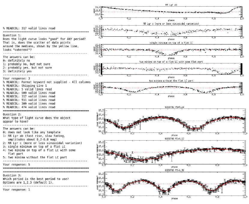
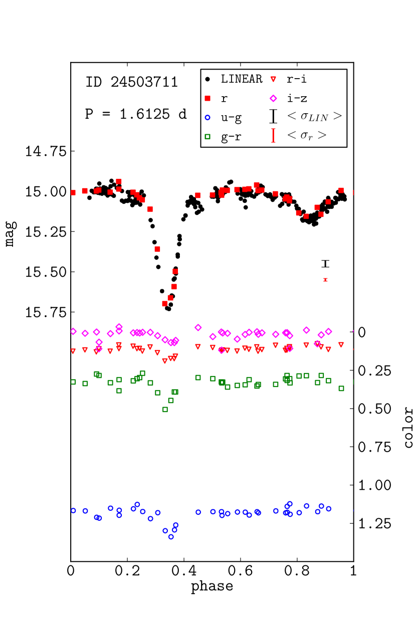
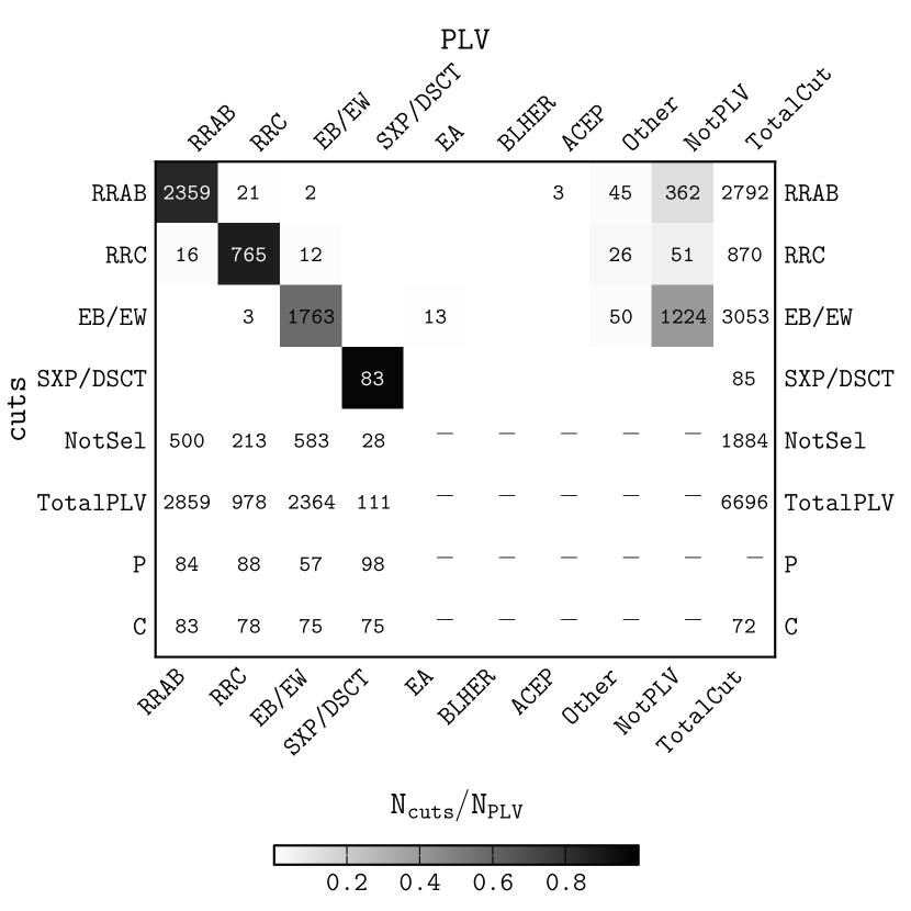
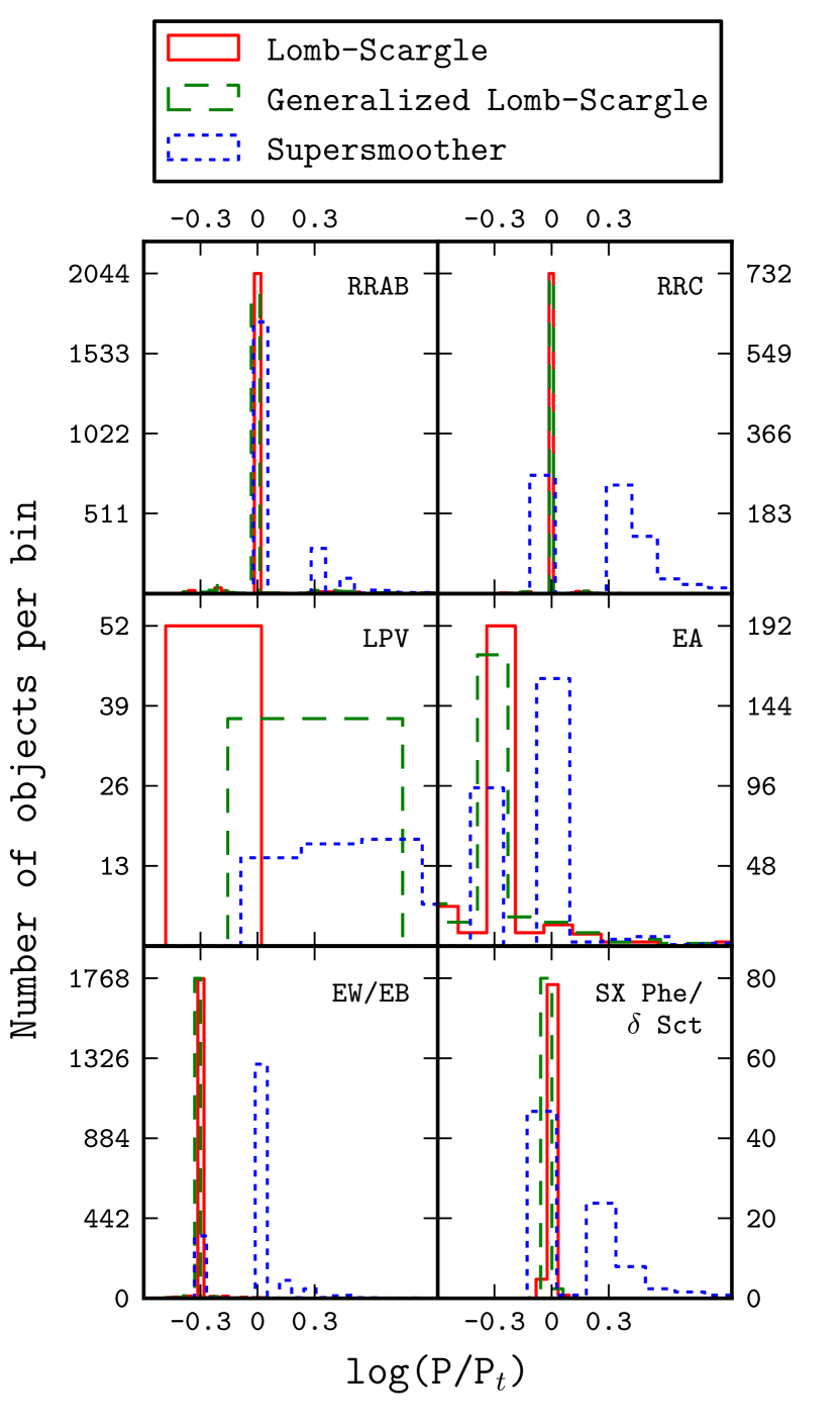
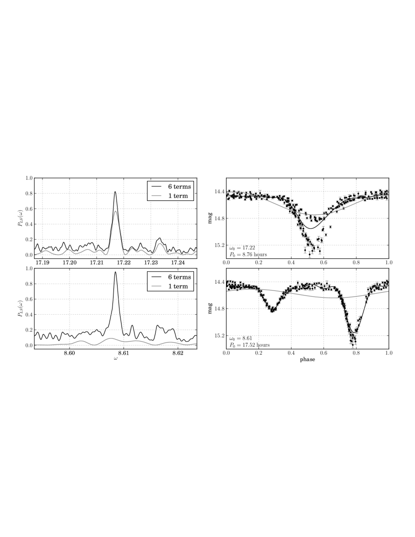
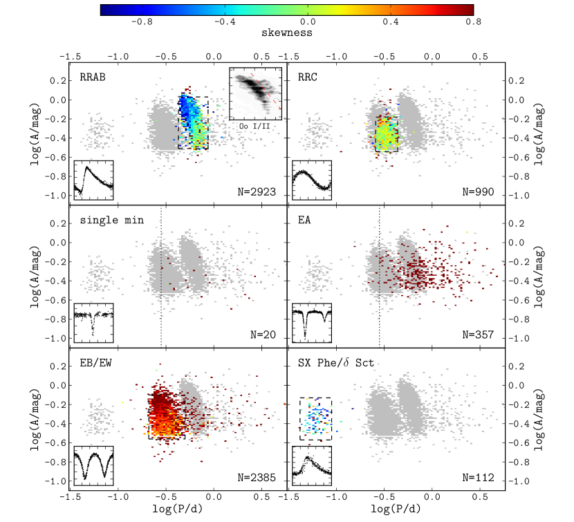
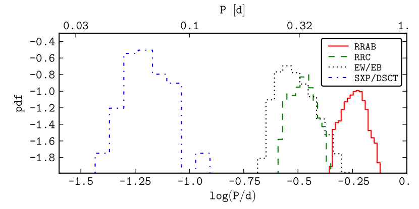
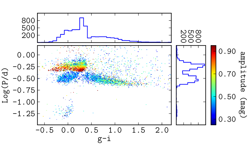
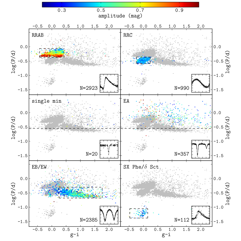
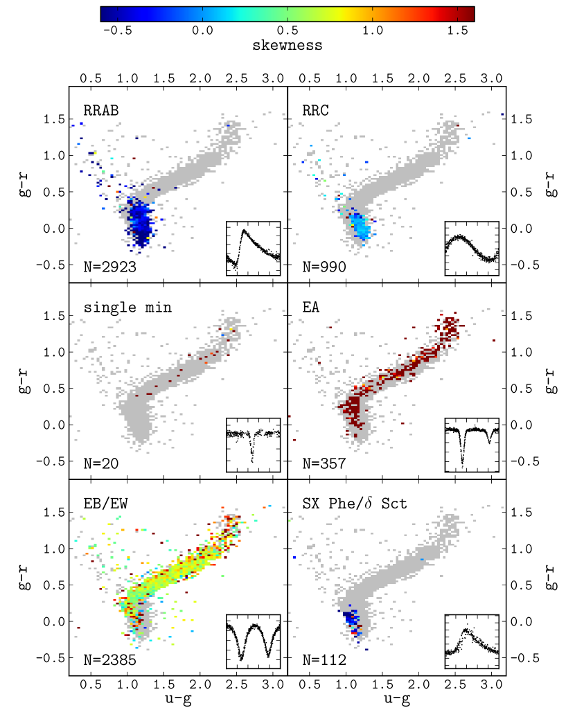
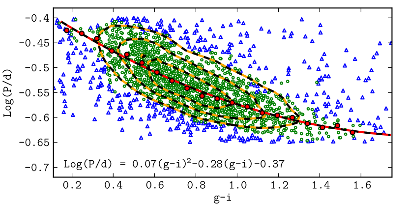
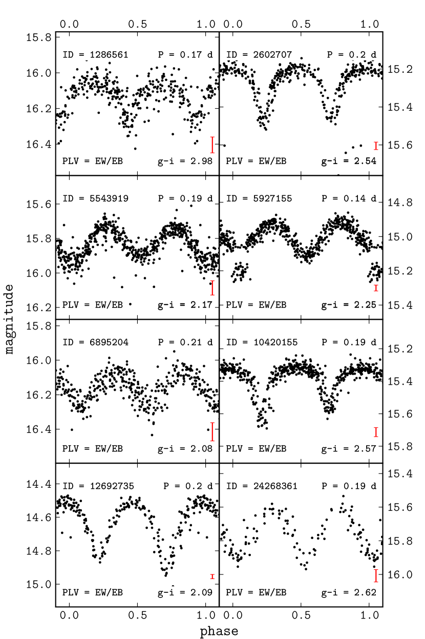
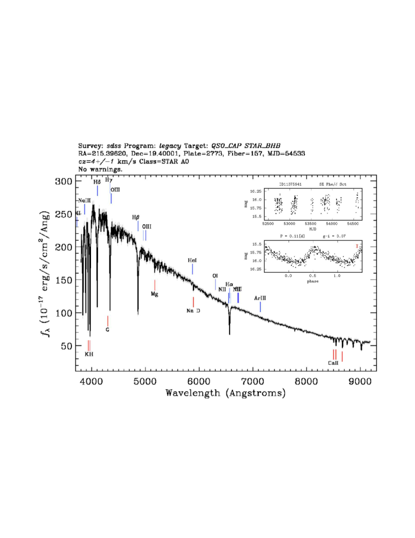
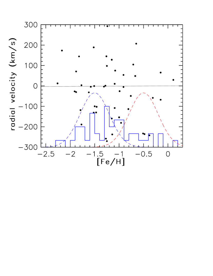
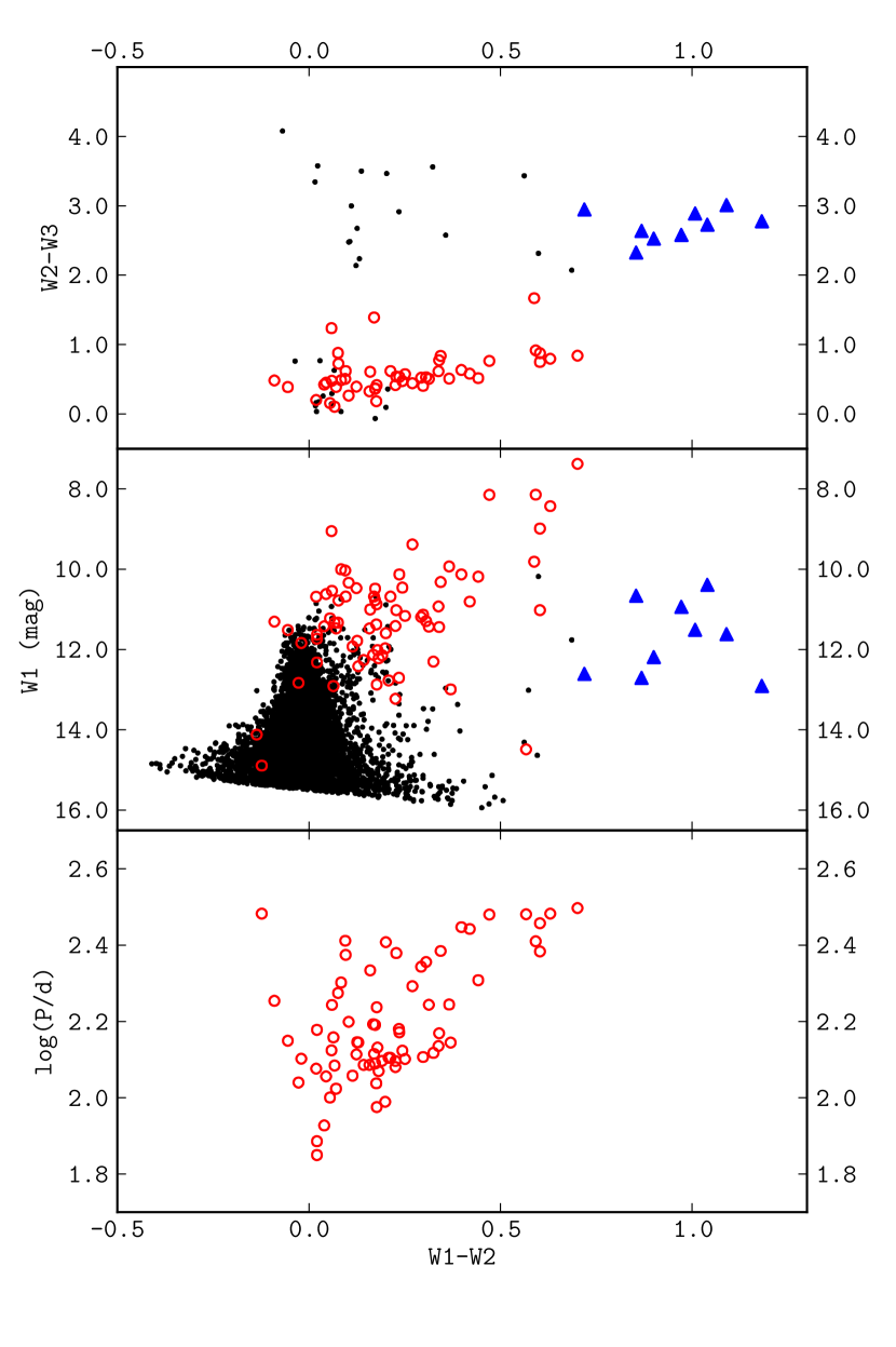
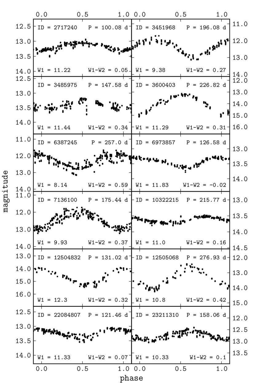
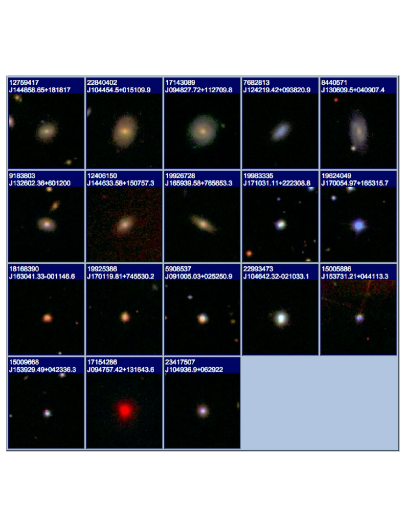
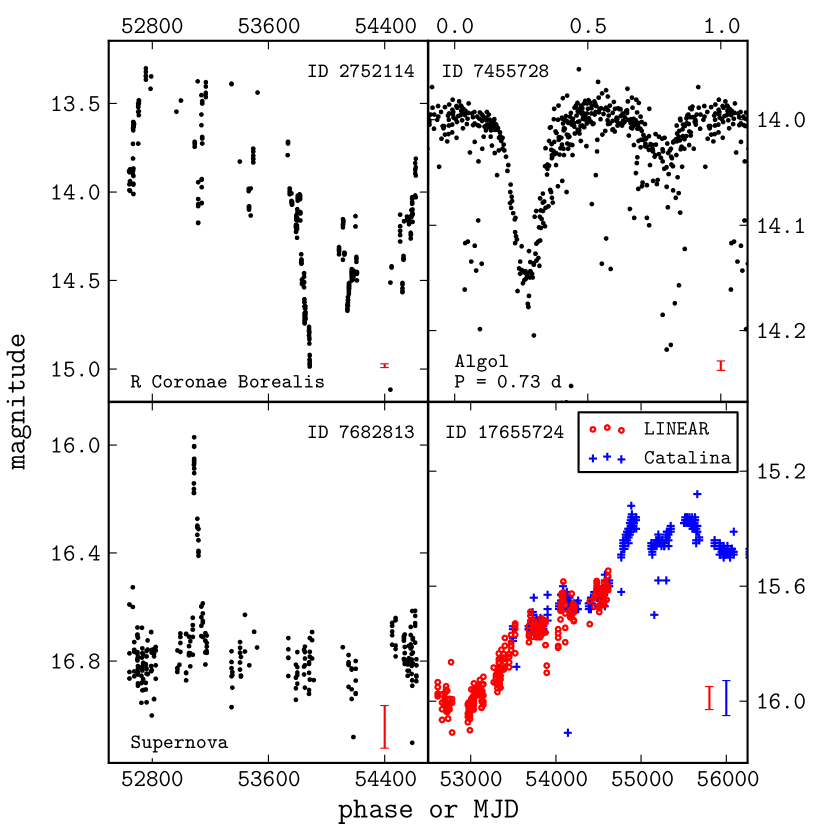
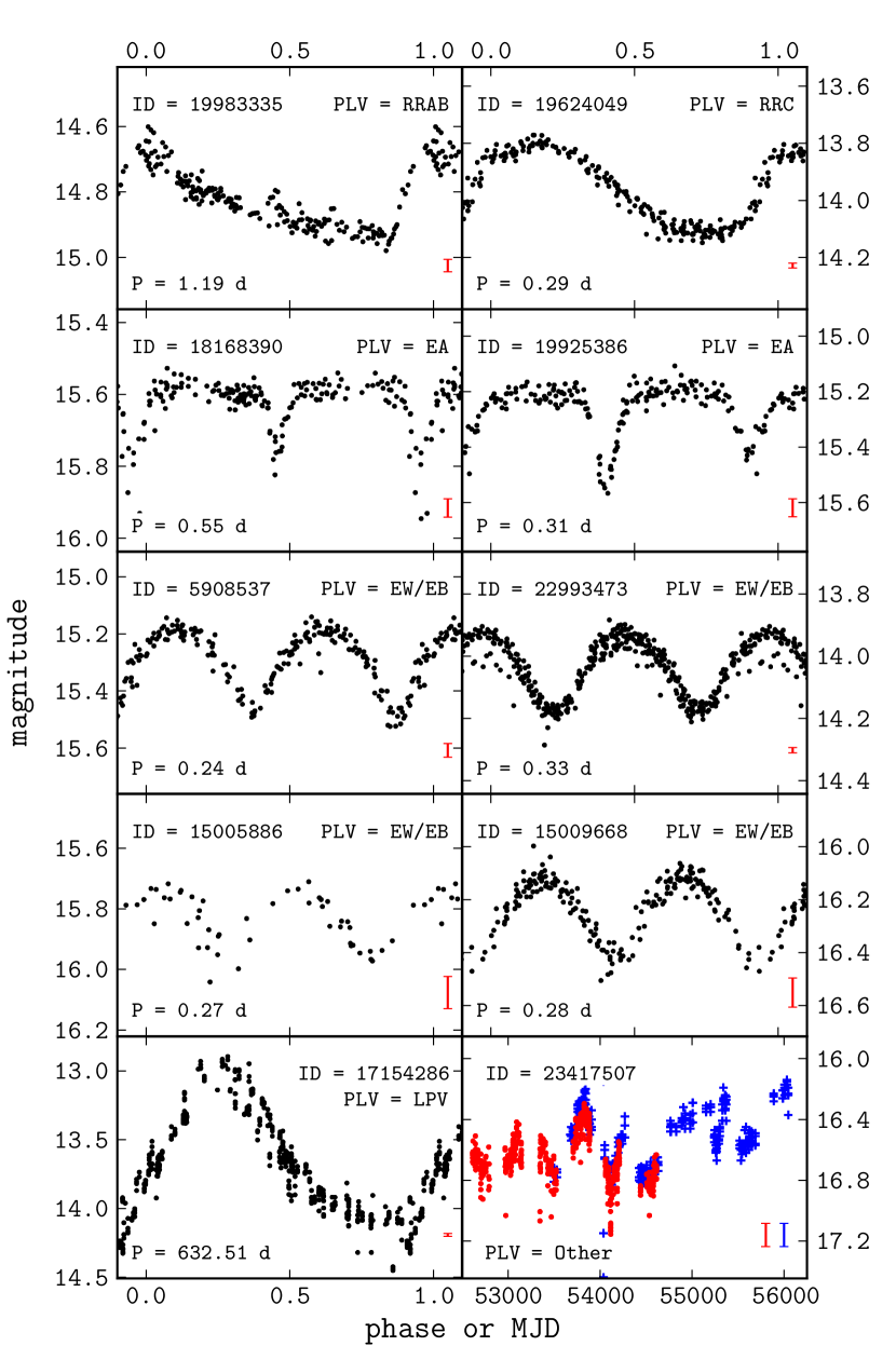
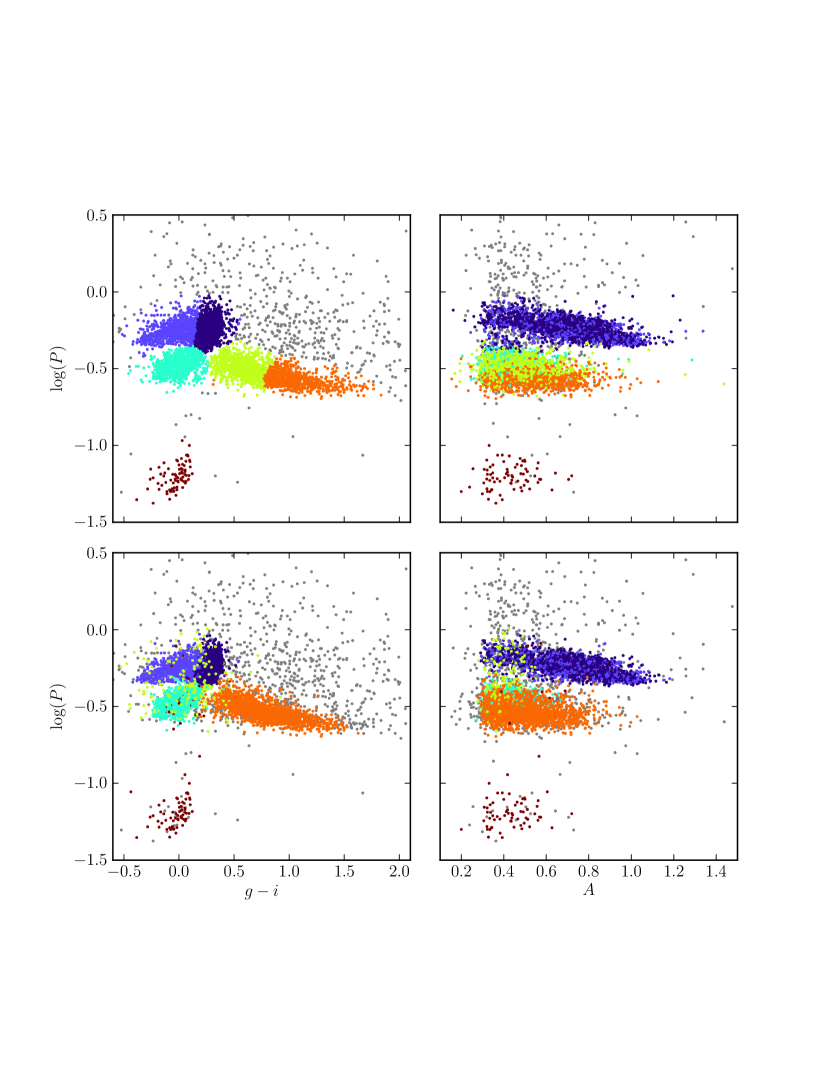
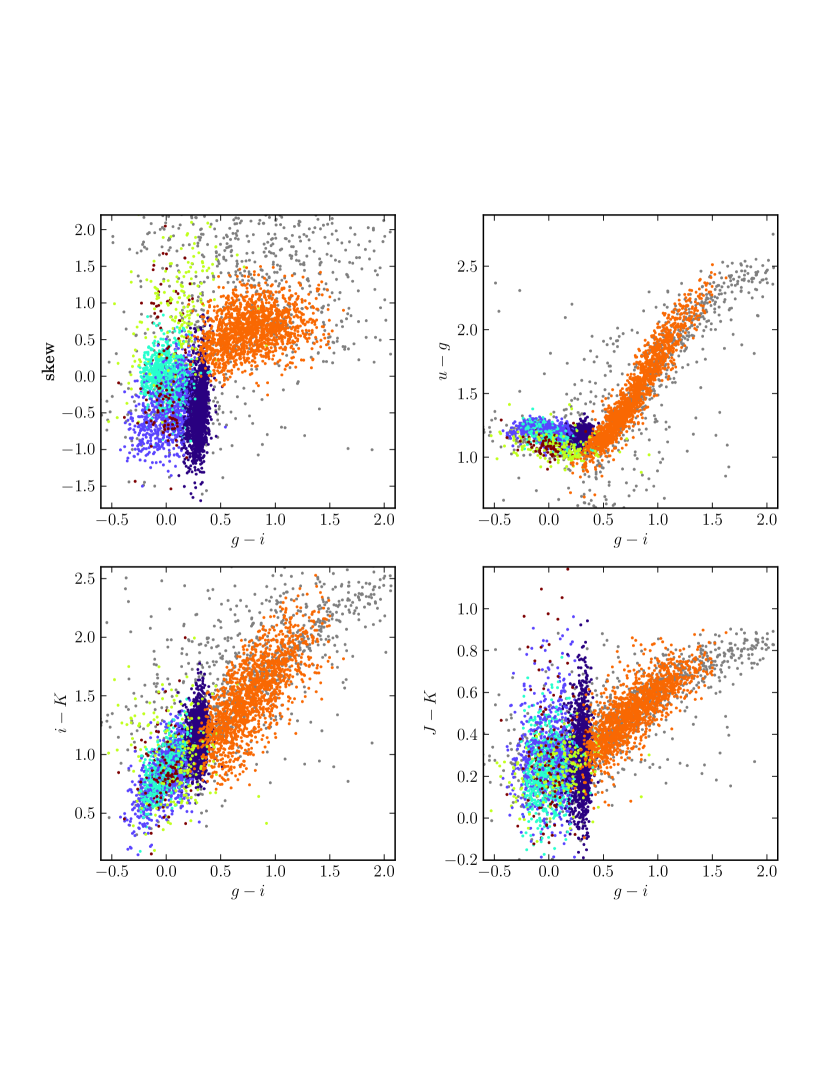
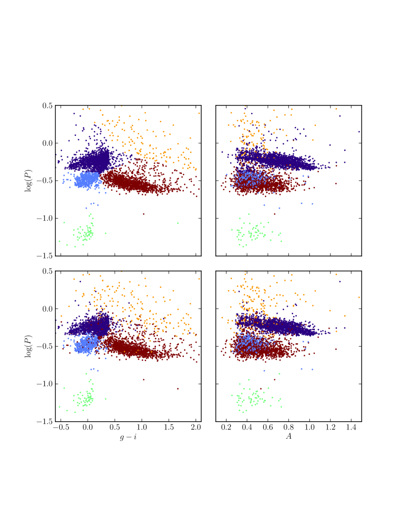
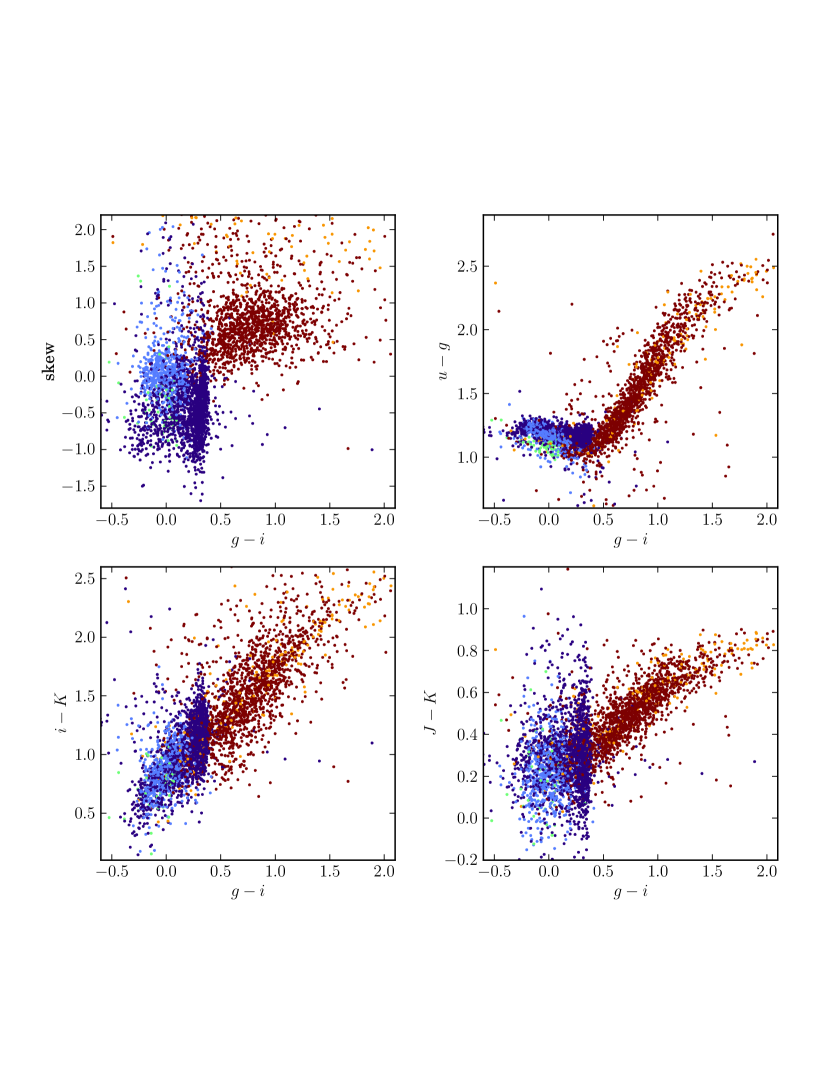
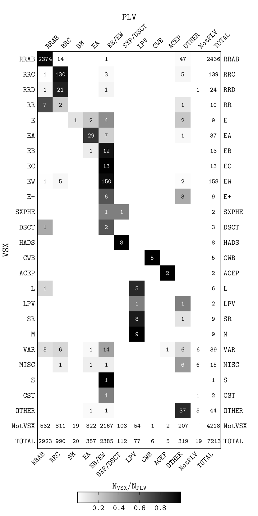
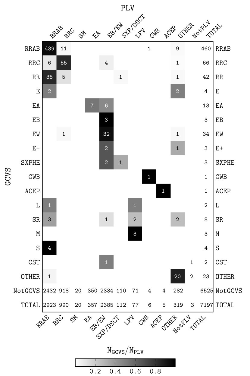
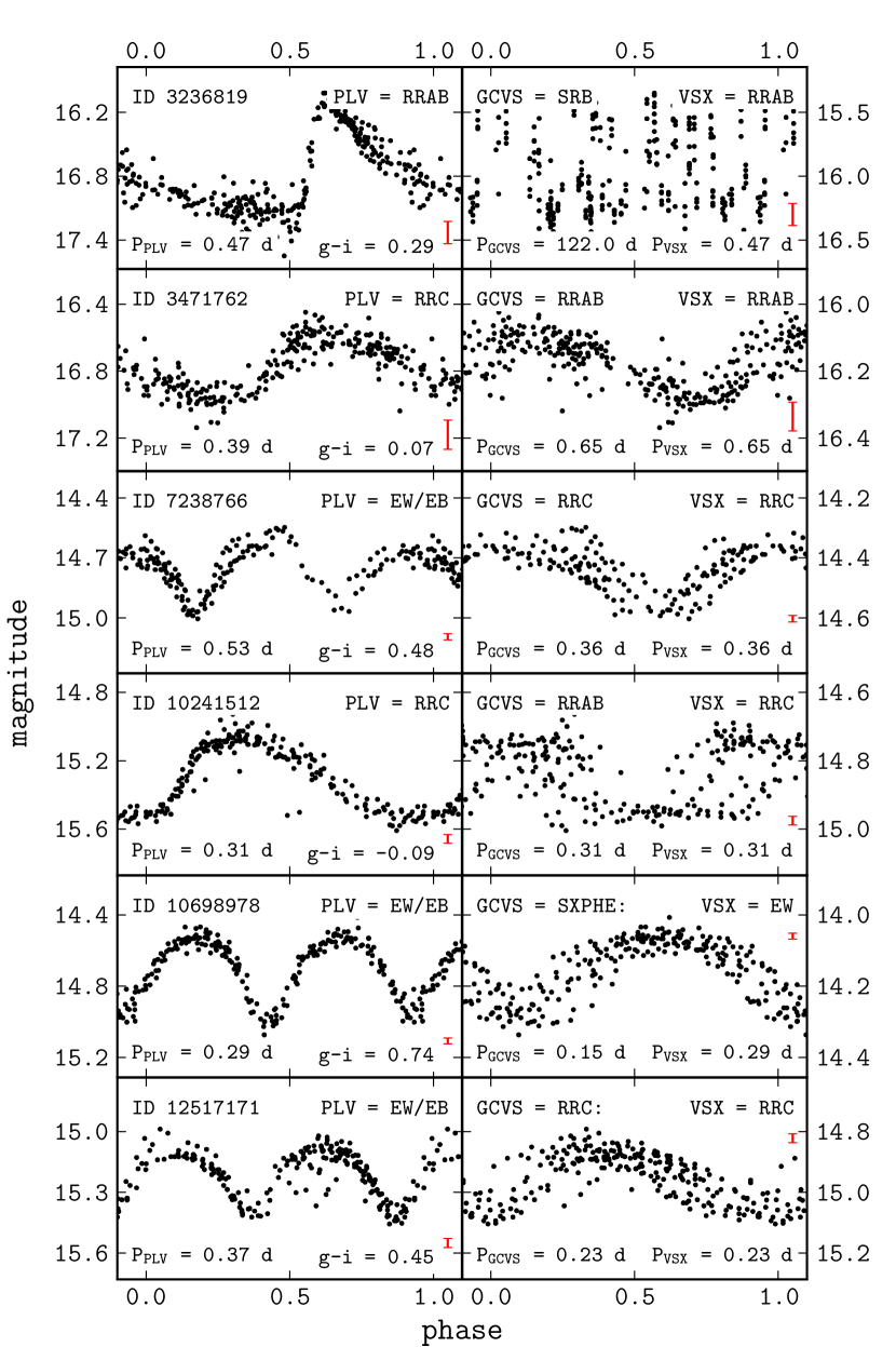
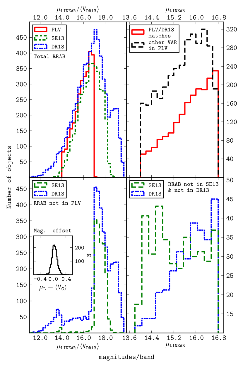
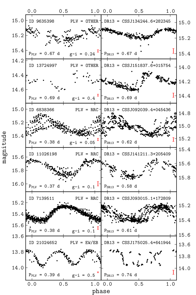
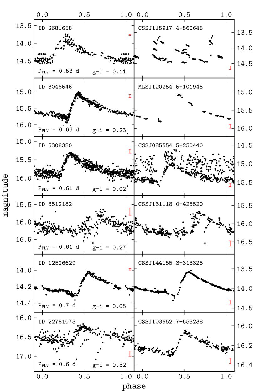
| Class | ||||||
|---|---|---|---|---|---|---|
| 0 | 0.0 | 1.1 | 0.38 | 7606 | 9.1 | 1.9 |
| 1 | 1.1 | 1.2 | 0.60 | 75 | 35.4 | 5.9 |
| 2 | 1.2 | 1.8 | 0.73 | 46 | 24.8 | 4.7 |
| 3 | 1.8 | 3.0 | 0.15 | 317 | 28.1 | 13.3 |
| Type | log(P) [d] | log(A) [mag] | skewness | g-i |
|---|---|---|---|---|
| ab RR Lyr | ||||
| c RR Lyr | ||||
| single min | ||||
| Algol | ||||
| Lyr & W UMa | ||||
| SX Phe/ Sct |
| Class | Type | F [%] | N |
|---|---|---|---|
| 1 | RRAB | 41 | 2923 |
| 2 | RRC | 14 | 990 |
| 3 | SM | 1 | 20 |
| 4 | EA | 5 | 357 |
| 5 | EB/EW | 33 | 2385 |
| 6 | SXP/DSCT | 2 | 112 |
| 7 | LPV | 1 | 77 |
| 8 | Hearbeat | 1 | 1 |
| 9 | BL Her | 1 | 6 |
| 11 | ACEP | 1 | 5 |
| 0 | Other | 4 | 318 |
| Total | 100 | 7194 |
| Class | N | RRAB | RRC | EA | EB/EW | SX Phe |
|---|---|---|---|---|---|---|
| RRAB | 1772 | 95.9 | 0.3 | 1.4 | 2.4 | 0.0 |
| RRC | 583 | 1.5 | 91.3 | 0.2 | 7.0 | 0.0 |
| EA | 228 | 5.3 | 1.3 | 67.5 | 25.9 | 0.0 |
| EB/EW | 1507 | 2.1 | 4.0 | 3.1 | 90.7 | 0.1 |
| SX Phe | 56 | 0.0 | 1.8 | 0.0 | 1.8 | 96.4 |
| Purity | 97 | 88.4 | 68.4 | 90.5 | 98.2 |
| ID | LCtype | P | A | mmed | stdev | rms | L | nObs | skew | kurt | L | CUF | t2 | t3 |
|---|---|---|---|---|---|---|---|---|---|---|---|---|---|---|
| 2522 | 5 | 0.238812 | 0.68 | 17.00 | 0.22 | 0.25 | 0.543 | 225 | 0.75 | 0.11 | 0.317 | 1 | 0 | 0 |
| ID | RA | Dec | oType | nS | rExt | u | g | r | i | z | uErr | gErr | rErr | iErr | zErr |
|---|---|---|---|---|---|---|---|---|---|---|---|---|---|---|---|
| 2522 | 117.99 | 48.67 | 6 | 1 | 0.139 | 20.24 | 18.24 | 17.28 | 16.89 | 16.67 | 0.06 | 0.01 | 0.01 | 0.01 | 0.01 |
| ID | J | H | K | Jerr | Herr | Kerr | W1 | W2 | W3 | W4 | W1err | W2err | W3err | W4err |
|---|---|---|---|---|---|---|---|---|---|---|---|---|---|---|
| 2522 | 15.45 | 14.94 | 14.76 | 0.06 | 0.09 | 0.10 | 14.52 | 14.63 | 12.60 | 8.84 | 0.03 | 0.07 | -9.90 | -9.90 |