Marangoni convection in an evaporating droplet: Analytical and numerical descriptions

Abstract

The stationary single vortex Marangoni convection in an axially symmetrical sessile drop of capillary size is considered. The detailed description of the fluid flows is presented for a wide range of contact angles, which takes into account the boundary conditions and the mass balance equation, without explicitly solving the Navier–Stokes equations. The analytical approach developed is compared with the results of numerical simulations and demonstrated to describe reasonably well the single-vortex Marangoni flows. This indicates the substantial role of the boundary conditions in the problem.

1 Introduction

The evaporation of a liquid droplet was studied since Maxwell time [2, 3, 4], and has attracted much attention over the last decade and a half in view of its role in various engineering applications, the advent of nanotechnology and progress in understanding of the evaporation process. In particular, the structure of the fluid flow produced by surface-tension-driven (Marangoni) instability inside an evaporating droplet has been intensively studied (see, for example, [5, 6] and references therein).

While numerical calculations of Marangoni convection agree well with corresponding experimental data [7, 8, 9], existing analytical studies of capillary flows in droplets are either limited to the case of small contact angles (see Sec. 2) or disregard Marangoni stresses at the droplet free surface [10, 11, 12]. Under the former conditions the problem is known to simplify and to be treated usually within the lubrication approximation. However, even in this case the analytical analysis of the Marangoni convection has been restricted up to now by its combination with a numerical fitting of the temperature distribution over a free droplet surface, which plays a key role as a source of the Marangoni effect. The latter approach can be valid when the Marangoni forces are suppressed due to effects of surface surfactants or for other reasons. However, generally, both the evaporative capillary flows and buoyancy-driven convection are much weaker than the Marangoni fluid flow for a droplet of capillary size [15, 14, 13], and the consideration of surface tension gradients is necessary. The primary purpose of this work is to study in detail the structure of Marangoni convection in evaporating droplets with pinned contact line, with an emphasis on the effects of the boundary conditions and the mass balance equations. It is demonstrated that the fluid flows can be obtained analytically for a wide range of contact angles, when the existing model of the droplet evaporation, known mainly from numerical studies, is formulated in a simplified manner.

In order to calculate the fluid dynamics in an evaporating sessile droplet, one has to solve numerically the coupled system of equations which contains the nonstationary vapor diffusion equation, the thermal conduction equation, the Navier–Stokes equations and to recalculate the droplet shape at each step due to the evaporative mass loss for the respective time interval [13]. The self-consistent solution should take into account an inhomogeneous evaporating flux density in the boundary conditions for the thermal conduction equation, since it is related to the heat transfer and hence to the temperature gradient at the droplet surface. The variation of temperature over the droplet surface affects the boundary conditions for the fluid dynamics, since the surface tension depends on temperature. In addition, the velocity field can influence the thermal conduction as a result of the effects of heat convection.

The calculations can be considerably simplified under the following conditions:

1. The capillary number ${\mathrm{Ca}}=\eta\overline{u}/\sigma$ and the Bond number ${\mathrm{Bo}}=\rho gh_{0}R/(2\sigma\sin\theta)$ are much smaller than unity (see the notations in Table 1). In this case, the sessile drop shape $h(r,t)$ can be approximated with high accuracy by the spherical cap approximation (see Fig. 1b)

   $$h(r,t)=\frac{R(\cos\phi(r,t)-\cos\theta(t))}{\sin\theta(t)};\qquad\phi(r,t)=\arcsin\left(\frac{r\sin\theta(t)}{R}\right).$$ (1)

   Here $\theta$ is the droplet contact angle, $\overline{u}$ is the characteristic velocity and $h_{0}=h(0,t)$ is the droplet height. The condition ${\mathrm{Ca}}\ll 1$ signifies that the viscous forces, which generally enter the boundary condition for the pressure, are much smaller than capillary forces, and the hydrostatic Young–Laplace equation can be used in order to determine the droplet shape. Under the condition ${\mathrm{Bo}}\ll 1$, influence of gravitational forces on the droplet shape is also small (see, for example, [13]).

2. The inverse Stanton number ${\mathrm{St}}^{-1}=\overline{u}R/\kappa$ is much smaller than unity. In this case the rate of the convective heat transfer is much smaller than conductive heat transfer, and, hence, the velocity field does not influence the thermal conduction (see, for example, [14]).

3. The transient time for heat transfer $t_{heat}=Rh_{0}/\kappa$, transient time for momentum transfer $t_{mom}=\rho Rh_{0}/\eta$ and transient time for vapor phase mass transfer $t_{mass}=\rho_{vap}/\rho_{f}\cdot t_{f}$ should be much smaller than the total drying time $t_{f}\approx 0.2\rho Rh_{0}/(Du_{s})$. This permits to describe the quasistationary stage of the evaporation process disregarding the time derivatives in the heat conduction equation, Navier–Stokes equation and the diffusion equation.

4. The dimensionless number $\rho gh^{2}\beta/(7\sigma^{\prime})$, where $\beta$ is thermal expansion coefficient, is much smaller than unity. In this case buoyancy-induced convection is much weaker than Marangoni flow [25].

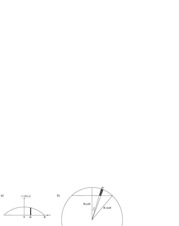
Figure 1: The droplet and its element in the $rz$- and in the ${n\tau}$-coordinate system correspondingly.

The laminar character of the flow should be also assumed. A turbulent regime arises in the droplet only for very large values of Marangoni and Reynolds numbers [26]. Therefore, the laminar character of the flow does not imply that the Reynolds number ${\mathrm{Re}}=\rho\overline{u}R/\eta$ is much smaller than unity. The condition b) specified above assumes that ${\mathrm{Re}}\cdot\nu/\kappa={\mathrm{St}}^{-1}$ is small. Since Prandtl number is greater than one for the majority of liquids, it follows from the condition that the Reynolds number is also assumed to be small. Nevertheless, most of the relations derived in the present paper are not directly connected to the calculation of the temperature distribution, and, therefore, are potentially applicable to the case of larger Reynolds numbers.

It is natural to start from the vapor diffusion equation, which can be solved independently from the other equations. We focus on so-called lens model of evaporation, which is consistent with the liquid–vapor interface at equilibrium and the evaporation limited by the diffusion of vapour into the surrounding gas. While other evaporative regimes are known in which the evaporation rate is controlled not by vapor diffusion but by phase change/kinetics processes at the interface (see, e.g., [27]), it is known that the diffusion-limited evaporation model agrees well with experimental data for moderately volatile droplets of capillary size with pinned contact line at atmospheric pressure of air and ambient temperature (see detailed discussions in, e.g., [6, 13, 17, 27, 31, 35]). In particular, an evaporation of a droplet deposited onto a heated substrate, where the atmospheric convective transport should be taken into account together with the diffusive model [28, 29, 30], is beyond the scope of the present paper. The analytical solution to the stationary vapor diffusion equation with appropriate boundary conditions gives the inhomogeneous evaporation flux from the surface of the evaporating droplet of a spherical shape [16]

$$J_{s}(r)=\frac{Du_{s}}{R}\left(\frac{\sin\theta}{2}+\sqrt{2}(x(r)+\cos\theta)^{3/2}\int_{0}^{\infty}\frac{\cosh(\theta\tau)}{\cosh(\pi\tau)}\tau\tanh((\pi-\theta)\tau)P_{-1/2+i\tau}(x(r))d\tau\right),$$ (2)

where $x(r)={\left(r^{2}\cos\theta/R^{2}+\sqrt{1-r^{2}\sin^{2}\theta/R^{2}}\right)}/{(1-r^{2}/R^{2})}$ and $P_{-1/2+i\tau}(x)$ is the Legendre polynomial. It was shown in [16] that (2) can be approximated with high accuracy as

$$J_{s}(r)=J_{0}(\theta)(1-r^{2}/R^{2})^{-\lambda(\theta)},$$ (3)

where $\lambda(\theta)=1/2-\theta/\pi$ and explicit expressions for $J_{0}(\theta)$ can be found in [17].

Under the condition b) specified above, the heat conduction equation inside the droplet can be solved independently, provided that the evaporation flux, which is connected to the temperature gradient at the droplet surface through the boundary condition $\partial T/\partial n=-LJ_{s}(r)/k$, is determined by (2). We obtain numerically the surface temperature distribution of the drop under the time independent conditions, which is justified by the quasistationarity of the evaporation process (see the condition c) above). We use a fitting procedure for a surface temperature which will be explained in more detail in Sec. 4. The following relation fits the obtained quasistationary temperature at the droplet surface with high accuracy, where the parameters $a$, $b$, $c$ and $\Delta T$ were placed in Table 2:

$$\frac{T}{\Delta T}=a\left(\frac{r}{R}\right)^{b}+(1-a)\left(\frac{r}{R}\right)^{2}+c.$$ (4)

Here $\Delta T$ is the temperature difference between the apex of the droplet and the substrate. The droplet and fluid properties in Table 1 were used during the numerical simulation.

For small contact angles the surface temperature distribution will be obtained analytically in Sec.2. This allows completely analytical description of the Marangoni convection in the lubrication approximation for an evaporating droplet, as distinct from the previous considerations in [15, 14].

The next step is the calculation of the fluid velocities in the droplet, where the obtained profile of the surface temperature enters the boundary condition at the droplet surface through the corresponding surface tension. It was found in [16, 15, 14] that this problem allows an approximate analytical description at least for the case of droplets with relatively small contact angles (see Sec. 2). The derivation of the analytical description of the fluid flow employs only the boundary conditions and the mass balance equations, without explicitly solving the Navier–Stokes equations.

For the analysis and interpretation of simulation results it is quite desirable to have a simplified description of the phenomenon, which nevertheless would be in a good agreement with the numerical data. In this paper we will generalize the existing analytical descriptions and will compare in detail the analytical and the numerical results for various droplets. We will describe how to accurately deal with the boundary conditions for this problem and how to obtain a number of additional conditions from the mass balance equations. We will find that a reasonable description of the fluid flows in a wide range of contact angles can be obtained taking into account the boundary conditions and the mass balance equations, without explicitly solving the Navier–Stokes equations. Instead of solving the Navier–Stokes equation, which is not known to have an analytical solution for such problem, we will use an appropriate approximation. The conditions a) – d) above are generally valid for a capillary size liquid drop, except that strong Marangoni flows in relatively large volatile droplets may transport heat rapidly enough that the convective heat transfer may not be negligible. The results are applicable when convective heat transfer is negligible, i.e. when ${\mathrm{St}}^{-1}=\overline{u}R/\kappa\ll 1$. Also, we focus on pinned contact line configuration and we only consider $\theta<90^{\circ}$. A moving contact line or contact angles larger than $90^{\circ}$ could lead to additional issues not being considered in the present work.

Sec. 2 represents a brief review of the lubrication approximation derived in [15, 14], completed with the analytical description of the corresponding surface temperature distibution and with further heuristic extension of the lubrication approximation. The new analytical description resulting in better accuracy is developed in Section 3. Sec. 4 contains discussion of the obtained analytical and numerical results.

2 The lubrication approximation

The lubrication approximation for an evaporating droplet of capillary size was derived in [15, 14]. The derivation includes three basic assumptions which are justified for $\theta\ll 1$:

1. The radial velocity $u_{r}(z)$ at each value of $r$ has a quadratic dependence on $z$.

2. The droplet free surface is approximated as a parabola $h(\tilde{r},t)=h(0,t)(1-\tilde{r}^{2})$, where $\tilde{r}=r/R$.

3. The total shear stress at the droplet free surface is approximated by the $rz$-component of the stress tensor.

Consider an axially symmetrical column in the droplet (see Fig. 1a). The mass balance equation states that the rate of mass change in the given volume element is equal to the net flux of mass into the element:

$$\frac{d}{dt}(\delta m)=-\oint\rho\,{\mathbf{u}}\cdot d{\mathbf{f}},$$ (5)

where the vector $d\mathbf{f}$ is perpendicular to the surface of the element, its absolute value is equal to the area of a small part of the boundary of the element, and the amount of mass which evaporates each second from the surface of the element is assumed to be also properly included in the surface integral in the right-hand side of (5). An easy consequence of the mass balance equation for the column was obtained in [16]:

$$\overline{u}_{r}(r,t)=-\frac{1}{\rho rh}\int_{0}^{r}dr\,r\left(J_{s}(r,t)\sqrt{1+\left(\frac{\partial h}{\partial r}\right)^{2}}+\rho\frac{\partial h}{\partial t}\right),$$ (6)

where $\overline{u}_{r}(r,t)$ is a height-averaged velocity in the column. Let $\tilde{r}=r/R$, $\tilde{z}=z/h_{0}$, $\tilde{u}_{r}=u_{r}t_{f}/R$, $\tilde{u}_{z}=u_{z}t_{f}/h_{0}$, $\tilde{t}=t/t_{f}$, $\tilde{h}=h(r)/h_{0}$, $M_{a}=-\sigma^{\prime}_{T}\Delta Tt_{f}/(\eta R)$, $\tilde{J}=-J_{0}/\rho{\dot{h}_{0}}$. Substituting in (6) the free surface of the droplet as a parabola $h(r,t)=h_{0}(t)(1-\tilde{r}^{2})$ and the corresponding relations $dh_{0}/dt=2(dm/dt)/(\rho\pi R^{2})\approx h_{0}/(t-t_{f})$, $dm/dt=\pi J_{0}R^{2}/(1-\lambda)$, Hu and Larson obtained in [15] the relation

$$\frac{\overline{u}_{r}t_{f}}{R}=\frac{1}{4\tilde{r}}\frac{1}{1-\tilde{t}}\left((1-\tilde{r}^{2})^{-\lambda}-(1-\tilde{r}^{2})\right).$$ (7)

This relation for the height-averaged velocity in evaporating droplets with relatively small contact angles is the basis for the lubrication approximation for the droplets. Using the above assumptions a), b), c) and Eq. (7), Hu and Larson derived the main lubrication equation for $u_{r}$, which takes the form

$$\tilde{u}_{r}=\frac{3}{8}\frac{1}{1-\tilde{t}}\frac{1}{\tilde{r}}\left[(1-\tilde{r}^{2})-(1-\tilde{r}^{2})^{-\lambda}\right]\left(\frac{\tilde{z}^{2}}{\tilde{h}^{2}}-2\frac{\tilde{z}}{\tilde{h}}\right)+\left[\frac{\tilde{r}h_{0}^{2}\tilde{h}}{R^{2}}\left(\tilde{J}\lambda(1-\tilde{r}^{2})^{-\lambda-1}+1\right)+\frac{M_{a}h_{0}\tilde{h}}{2R}\frac{d\tilde{T}}{d\tilde{r}}\right]\left(\frac{\tilde{z}}{\tilde{h}}-\frac{3}{2}\frac{\tilde{z}^{2}}{\tilde{h}^{2}}\right)$$ (8)

and implies $\tilde{h}(\tilde{r},\tilde{t})=\tilde{h}_{0}(\tilde{t})(1-\tilde{r}^{2})$. As seen, $\tilde{u}_{r}(\tilde{r},\tilde{z})$ is the quadratic function of $\tilde{z}$ that can be considered as a result of expansion in powers of small parameter $\tilde{z}$ for droplets with small contact angles. Eq. (8) is applicable for arbitrary function $T(r)$ and at the same time it coincides with Eq. (28) in [14] provided that the surface temperature distribution is described by Eq. (4).

The final step of the derivation in [15, 14] is to find $\tilde{u}_{z}$ using the obtained $\tilde{u}_{r}$ and the continuity equation for the incompressible fluid. Here we represent the result in the form

$$\tilde{u}_{z}=\frac{3}{4}\frac{1}{1-\tilde{t}}\left(1+\lambda(1-\tilde{r}^{2})^{-1-\lambda}\right)\left(\frac{\tilde{z}^{3}}{3\tilde{h}^{2}}-\frac{\tilde{z}^{2}}{\tilde{h}}\right)-\frac{3}{4}\frac{1}{1-\tilde{t}}\left[(1-\tilde{r}^{2})-(1-\tilde{r}^{2})^{-\lambda}\right]\left(\frac{\tilde{z}^{2}}{2\tilde{h}^{2}}-\frac{\tilde{z}^{3}}{3\tilde{h}^{3}}\right)\frac{1}{\tilde{r}}\frac{\partial\tilde{h}}{\partial\tilde{r}}-\\ -\frac{h_{0}^{2}}{R^{2}}\left(\tilde{J}\lambda(1-\tilde{r}^{2})^{-\lambda-1}+1\right)\left(\tilde{z}^{2}-\frac{\tilde{z}^{3}}{\tilde{h}}\right)-\frac{\tilde{r}^{2}h_{0}^{2}}{R^{2}}\tilde{J}\lambda(\lambda+1)(1-\tilde{r}^{2})^{-2-\lambda}\left(\tilde{z}^{2}-\frac{\tilde{z}^{3}}{\tilde{h}}\right)-\\ -\frac{\tilde{r}h_{0}^{2}}{R^{2}}\left(\tilde{J}\lambda(1-\tilde{r}^{2})^{-\lambda-1}+1\right)\frac{\tilde{z}^{3}}{2\tilde{h}^{2}}\frac{\partial\tilde{h}}{\partial\tilde{r}}-\frac{M_{a}h_{0}}{4R}\left(\frac{d^{2}\tilde{T}}{d\tilde{r}^{2}}+\frac{1}{\tilde{r}}\frac{d\tilde{T}}{d\tilde{r}}\right)\left(\tilde{z}^{2}-\frac{\tilde{z}^{3}}{\tilde{h}}\right)-\frac{M_{a}h_{0}}{4R}\frac{d\tilde{T}}{d\tilde{r}}\frac{\tilde{z}^{3}}{\tilde{h}^{2}}\frac{\partial\tilde{h}}{\partial\tilde{r}}.$$ (9)

Substituting $\tilde{h}(\tilde{r},\tilde{t})=\tilde{h}_{0}(\tilde{t})(1-\tilde{r}^{2})$ and (4) in Eq. (9), one obtains Eq. (29) in [14]. The assumption $\tilde{h}(\tilde{r},t)=\tilde{h}_{0}(t)(1-\tilde{r}^{2})$ is inherent to the lubrication approximation and, in particular, to Eq. (7) above and to Eqs. (28) and (29) in [14].

The temperature distribution can be obtained analytically for $\theta\ll 1$. Indeed, the boundary conditions for the temperature distribution take the form $\partial T/\partial r=0$ for $r=0$; $T=T_{0}$ for $z=0$; ${\partial T}/{\partial n}=-LJ_{s}(r)/k$ at the drop surface. In particular, for $r=0$ we have $\left(\partial T/\partial z\right)_{r=0}=-LJ_{0}/k=-\Delta T/h_{0}$, therefore, $\Delta T=LJ_{0}h_{0}/k$. For small contact angles one can approximate the boundary condition at the surface as ${\partial T}/{\partial z}=-LJ_{s}(r)/k$. Therefore, using (1) and (3), one obtains the surface temperature distribution:

$$\frac{T}{\Delta T}=\frac{T_{0}}{\Delta T}-\frac{LJ_{s}(r)h(r)}{k\Delta T}=\frac{T_{0}}{\Delta T}-\frac{J_{s}(r)h(r)}{J_{0}h_{0}}=\frac{T_{0}}{\Delta T}-\left(1-\frac{r^{2}}{R^{2}}\right)^{1/2+\theta/\pi}.$$ (10)

For small contact angles the rate of mass loss is $-dm/dt=-\rho\pi R^{3}\theta^{\prime}(t)/4=2\pi J_{0}(\theta)R^{2}$, hence one can estimate $J_{0}$ and $\Delta T$ as follows: $J_{0}(\theta)=-\rho R\theta^{\prime}(t)/8$ and $\Delta T=LJ_{0}h_{0}/k=-\rho R^{2}\theta\theta^{\prime}(t)L/(16k)$. Eq. (10) obtained here agrees well with the numerical simulations for small contact angles.

The main purpose of this work is to develop analytical description of fluid flows in an evaporating droplet in a wide range of contact angles. As a first step, we will test the heuristic extension of the lubrication approximation, substituting in Eqs. (8) and (9) the functions $\tilde{h}(\tilde{r})$ and $\partial\tilde{h}/\partial\tilde{r}$, which are obtained from (1), i.e., which correspond to the spherical cap profile of the sessile drop. The equations were written in the form of Eqs. (8) and (9) in order to represent heuristic description for larger contact angles, where $h(r)$ is substantially nonparabolic. This improves the accuracy for larger contact angles, without changing the solution for small contact angles. We note that the continuity equation is precisely satisfied for arbitrary $h(r)$ and $T(r)$, if $\tilde{u}_{r}$ and $\tilde{u}_{z}$ are represented in the form (8), (9), as opposed to the original form of lubrication equations, where the continuity equation is satisfied for small contact angles. We formulate and use the heuristic extension to larger contact angles for comparison with more consistent results obtained in this work.

3 Derivation of the description in the $n\tau$ -coordinate system

In this section the analytical approach for calculating the fluid velocities in an evaporating droplet will be consistently and explicitly developed without using the assumptions $a),b),c)$ of Section 2. The boundary conditions at the droplet surface will be considered assuming its spherical profile.

Consider the spherical $n\tau$-coordinate system, where $n$ is the distance between a point inside the droplet and the center of the sphere which contains the droplet surface, $\phi$ is the azimuthal angle, and $\tau=n\phi$ (see Fig. 1b). The notation was taken to emphasize that the coordinates correspond to the normal and tangential directions to the droplet surface. Therefore, at the substrate we have $n=n_{1}=R\cot\theta/\cos\phi$, and at the droplet surface we have $n=n_{2}=R/\sin\theta$. The $n\tau$-coordinates are connected with the cylindrical $rz$-coordinates via the following relations: $r=n\sin\phi$; $z=n\cos\phi-R\cot\theta$; $n=\sqrt{r^{2}+(z+R\cot\theta)^{2}}$; $\tau=n\phi$; $\phi=\arcsin(r/n)$. Here $\theta$ is the contact angle, therefore $\phi\leq\theta$ for arbitrary point inside the droplet.

The total mass of the shaded element in Fig. 1b is

$$\delta m=\rho\int_{n_{1}}^{n_{2}}2\pi r(n)d\tau(n)dn=2\pi\rho\int_{n_{1}}^{n_{2}}(n\sin\phi)(nd\phi)dn=\frac{2}{3}\pi\rho\frac{R^{3}\sin\phi\cdot d\phi}{\sin^{3}\theta(t)}\left(1-\frac{\cos^{3}\theta(t)}{\cos^{3}\phi}\right).$$ (11)

The volume element is characterized by a fixed value of $\phi$, while the center of the sphere is moving in a downward direction during the evaporation process. Therefore, the element is also moving and the velocity of the element is $-R\theta^{\prime}(t)\sin\phi/\sin^{2}\theta$. It follows from the mass balance equation (5) for the element that

$$\frac{d}{dt}(\delta m)=-J_{s}(\tau,t)\cdot 2\pi(n_{2}\sin\phi)d\tau-2\pi\rho\cdot d\phi\frac{d}{d\phi}\left(\sin\phi\int_{n_{1}}^{n_{2}}n\left(u_{\tau}+\frac{R\theta^{\prime}(t)\sin\phi}{\sin^{2}\theta}\right)dn\right),$$ (12)

where $J_{s}$ can be obtained with (3). Hence one obtains the following relation for $I(\phi)=\int_{n_{1}}^{n_{2}}nu_{\tau}dn$:

$$I(\phi)=\frac{-R^{2}}{\sin^{2}\theta\sin\phi}\int_{0}^{\phi}\left(\frac{J_{0}}{\rho}\left(1-\frac{\sin^{2}\phi}{\sin^{2}\theta}\right)^{-\lambda}+\frac{R\cos\theta\cdot\theta^{\prime}(t)}{\sin^{2}\theta}\left(\frac{\cos\theta}{\cos^{3}\phi}-1\right)\right)\sin\phi\cdot d\phi-\frac{R^{3}\theta^{\prime}(t)\sin\phi}{2\sin^{4}\theta}\left(1-\frac{\cos^{2}\theta}{\cos^{2}\phi}\right).$$ (13)

Here one can use the approximation $\theta^{\prime}(t)\approx\theta/t_{f}$, where $t_{f}(t)$ is remaining time of evaporation. Indeed, the contact angle diminishes almost linearly with time during the evaporation process [13]. Eq. (13) results in the singularity in $u_{\tau}$ at the contact line, where $n_{1}(\phi)\to n_{2}$, which is a consequence of the singularity in evaporation rate at the contact line. Similar singularity problems are known for all known analytical models. In particular, the singularity enters Eqs. (6)–(9). The singularity can be regularized by introducing a disjoining pressure and/or precursor film [19, 20], by introducing a Navier slip [21, 20, 22] or by taking into account the Kelvin effect [23, 24]. The singularity influences the velocity field only in a small vicinity of the contact line and its detailed discussion is beyond the scope of the present paper.

At the droplet surface we have the following boundary condition (see Appendix B in [13]):

$$\frac{d\sigma}{\eta d\tau}=-\frac{M_{a}\cos\phi}{t_{f}}\frac{d\tilde{T}}{d\tilde{r}}=\frac{\partial u_{\tau}}{\partial n}+\frac{\partial u_{n}}{\partial\tau}-u_{\tau}\frac{d\phi}{d\tau}.$$ (14)

This very important boundary condition takes into account Marangoni forces associated with the temperature dependence of the surface tension, which generate fluid convection in the sessile drop. Additional condition at the droplet surface can be derived from the continuity equation:

$$\frac{u_{n}}{\cos\phi}=u_{r}\tan\phi+u_{z}=-u_{r}h^{\prime}(r)-\frac{1}{r}\int_{0}^{h(r)}\frac{\partial(ru_{r})}{\partial r}dz=-\frac{1}{r}\frac{\partial(rh\overline{u}_{r})}{\partial r},$$ (15)

hence, using the relation (6), one obtains at the droplet surface

$$u_{n}=\frac{\partial h(r,t)}{\partial t}\cos\phi+\frac{J_{0}(\theta)}{\rho}\left(1-\frac{\sin^{2}\phi}{\sin^{2}\theta}\right)^{-\lambda(\theta)}.$$ (16)

Substituting (1) in (16), one gets

$$u_{n} = \frac{R(\cos\phi-\cos\theta)\theta^{\prime}(t)}{\sin^{2}\theta}+\frac{J_{0}}{\rho}\left(1-\frac{\sin^{2}\phi}{\sin^{2}\theta}\right)^{-\lambda},$$ (17)

$$\frac{\partial u_{n}}{\partial\tau} = \frac{\sin\theta}{R}\frac{\partial u_{n}}{\partial\phi}=\frac{\sin\phi}{R\sin\theta}\left(\frac{2J_{0}\lambda\cos\phi}{\rho}\left(1-\frac{\sin^{2}\phi}{\sin^{2}\theta}\right)^{-\lambda-1}-R\theta^{\prime}(t)\right).$$ (18)

We will use the following approximation for $u_{\tau}$:

$$u_{\tau}(n,\phi)=(n-n_{1})^{p(\phi)}A(\phi)+(n-n_{1})B(\phi).$$ (19)

Here $p(\phi)$ is a trial function. The approach reasonably works for various trial functions $p(\phi)$. We will choose $p(\phi)$ in Section 4. The coefficient functions $A(\phi)$ and $B(\phi)$ will be specified based on the boundary condition (14) and the mass balance relation (13). Eq. (19) automatically satisfies the no-slip boundary condition at the substrate and, at the same time, allows the existence of a single vortex in a droplet.

Using (19), Eq. (14) can be rewritten as

$$A(\phi)(n_{2}-n_{1})^{p(\phi)-1}\left(p(\phi)-1+\frac{n_{1}}{n_{2}}\right)+B(\phi)\frac{n_{1}}{n_{2}}+\frac{\partial u_{n}}{\partial\tau}+\frac{M_{a}\cos\phi}{t_{f}}\frac{d\tilde{T}}{d\tilde{r}}=0,$$ (20)

where the right side of (18) can be used instead of ${\partial u_{n}}/{\partial\tau}$.

Eq. (13) gives the second linear relationship between $A(\phi)$ and $B(\phi)$:

$$\frac{A(\phi)}{(p+1)(p+2)}(n_{2}-n_{1})^{p+1}(n_{2}(p+1)+n_{1})+\frac{1}{6}B(\phi)(n_{2}-n_{1})^{2}(n_{1}+2n_{2})=I(\phi).$$ (21)

We note that the integral in the right side of (13) can be obtained exactly, because

$$\int_{0}^{\phi}\sin\phi\left(\frac{\cos\theta}{\cos^{3}\phi}-1\right)d\phi=\cos\phi-1+\frac{1}{2}\cos\theta\tan^{2}\phi,$$ (22)

$$\int\sin\phi\left(1-\frac{\sin^{2}\phi}{\sin^{2}\theta}\right)^{-\lambda}d\phi=(\cos\theta+\cos\phi)\left(1-\frac{\sin^{2}\phi}{\sin^{2}\theta}\right)^{-\lambda}{}_{2}F_{1}\left(1,\lambda;2\lambda;\frac{2\cos\theta}{\cos\theta-\cos\phi}\right)\frac{\Gamma(2\lambda-1)}{\Gamma(2\lambda)}+C,$$ (23)

where ${}_{2}F_{1}(a,b;c;z)$ is the hypergeometric function and $\Gamma(z)$ is the gamma function. Therefore,

$$I(\phi)=\frac{-R^{2}J_{0}}{\rho\sin^{2}\theta\sin\phi}(\cos\theta+\cos\phi)\left(1-\frac{\sin^{2}\phi}{\sin^{2}\theta}\right)^{-\lambda}{}_{2}F_{1}\left(1,\lambda;2\lambda;\frac{2\cos\theta}{\cos\theta-\cos\phi}\right)\frac{\Gamma(2\lambda-1)}{\Gamma(2\lambda)}+\\ +\frac{R^{2}J_{0}(\cos\theta+1)}{\rho\sin^{2}\theta\sin\phi}{}_{2}F_{1}\left(1,\lambda;2\lambda;\frac{2\cos\theta}{\cos\theta-1}\right)\frac{\Gamma(2\lambda-1)}{\Gamma(2\lambda)}+\frac{R^{3}\cos\theta\cdot\theta^{\prime}(t)}{\sin^{4}\theta\sin\phi}\left(1-\cos\phi-\frac{\sin^{2}\phi}{2\cos\theta}\right).$$ (24)

The quantity $I(\phi)$ is typically negligibly small. In particular, it is negligibly small for all droplets considered in Table 1 and $I(\phi)=0$ can be used in order to simplify the equations, because the evaporative-driven flows and the flows due to the nonzero value of $\theta^{\prime}(t)$ are tiny compared to the flow due to the Marangoni forces. The calculations confirm that for describing the Marangoni convection, the value of $I(\phi)$ could be replaced by zero almost without losing the accuracy. The quantity $I(\phi)$ and Eq. (24) could play an important role for describing the evaporative-driven flows in other situations, when the Marangoni forces are suppressed. For this reason, we will retain the quantity $I$ in the formulae. The calculations also show that the effect of nonzero $u_{n}$ and $\partial u_{n}/\partial\tau$ on the fluid flows (see Eqs.(17) and (18)) is quite small compared to the effect of Marangoni forces. Hence $\partial u_{n}/\partial\tau=0$ can be used in order to further simplify the equations. Still, we will retain $\partial u_{n}/\partial\tau$ in the formulae, because it could possibly be useful in situations involving extremely volatile liquids and a very fast evaporation.

Eqs. (20),(21) are the system of two linear relationships between $A(\phi)$ and $B(\phi)$. The solution is:

$$A=-\frac{(-n_{1}+n_{2})^{-1-p}(1+p)(2+p)\left(\left(6In_{1}+\frac{\partial u_{n}}{\partial\tau}(n_{1}-n_{2})^{2}n_{2}(n_{1}+2n_{2})\right)t_{f}+\frac{\partial\tilde{T}}{\partial\tilde{r}}M_{a}(n_{1}-n_{2})^{2}n_{2}(n_{1}+2n_{2})\cos\phi\right)}{(p-1)\left(2n_{2}^{2}(p+1)(p+2)+n_{1}^{2}(p+4)+n_{1}n_{2}(p+1)(p+4)\right)t_{f}},$$ (25)

$$B=\frac{6\left(I(p+1)(p+2)(n_{1}+n_{2}(p-1))t_{f}+(n_{1}-n_{2})^{2}n_{2}(n_{1}+n_{2}(p+1))((\partial u_{n}/\partial\tau)t_{f}+(\partial\tilde{T}/\partial\tilde{r})M_{a}\cos\phi)\right)}{(n_{1}-n_{2})^{2}(p-1)\left(2n_{2}^{2}(p+1)(p+2)+n_{1}^{2}(p+4)+n_{1}n_{2}(p+1)(p+4)\right)t_{f}}.$$ (26)

In order to complete the approximate analytical description of the velocity field, we need to obtain $u_{n}(n,\phi)$ inside the droplet. The continuity equation for the incompressible fluid $\mathrm{div}\,\mathbf{u}=0$ takes the following form in the $n\tau$-coordinate system:

$$\frac{\partial u_{n}}{\partial n}+\frac{2u_{n}}{n}+\frac{\partial u_{\tau}}{\partial\tau}+\frac{\cot\phi}{n}u_{\tau}=0.$$ (27)

Therefore,

$$\frac{1}{n}\frac{\partial(n^{2}u_{n}(n,\phi))}{\partial n}=-\frac{\partial u_{\tau}}{\partial\phi}-u_{\tau}\cot\phi=-A^{\prime}(\phi)(n-n_{1})^{p(\phi)}-B^{\prime}(\phi)(n-n_{1})+\\ +B(\phi)(n_{1}^{\prime}(\phi)-(n-n_{1})\cot\phi)+A(\phi)p(\phi)n_{1}^{\prime}(\phi)(n-n_{1})^{p(\phi)-1}-A(\phi)(n-n_{1})^{p(\phi)}(p^{\prime}(\phi)\log(n-n_{1})+\cot\phi),$$ (28)

$$u_{n}(n,\phi)=-\frac{A^{\prime}(\phi)(n-n_{1})^{p+1}}{n^{2}}\frac{n_{1}+np+n}{(p+1)(p+2)}-\frac{B^{\prime}(\phi)}{6n^{2}}(n-n_{1})^{2}(n_{1}+2n)+\frac{B(\phi)}{2n^{2}}(n^{2}-n_{1}^{2})n_{1}^{\prime}(\phi)-\\ -\frac{B(\phi)(2n+n_{1})(n-n_{1})^{2}\cot\phi}{6n^{2}}+\frac{A(\phi)(pn+n_{1})(n-n_{1})^{p}n_{1}^{\prime}(\phi)}{(p+1)n^{2}}-\frac{A(\phi)\cot\phi}{(p+1)(p+2)}\frac{(n_{1}+np+n)(n-n_{1})^{p+1}}{n^{2}}+\\ +\frac{A(\phi)p^{\prime}(\phi)(n-n_{1})^{p+1}}{n^{2}}\left(\frac{n}{(p+2)^{2}}+\frac{n_{1}(2p+3)}{(p+1)^{2}(p+2)^{2}}-\frac{(n+n_{1}+np)\log(n-n_{1})}{(p+1)(p+2)}\right).$$ (29)

Therefore, we have obtained the velocity field in the droplet: $u_{\tau}$ and $u_{n}$ are defined by (19) and (29), where $A(\phi)$ and $B(\phi)$ are determined by (25) and (26). The velocities in the cylindrical $rz$-coordinate system can be obtained from the known values of $u_{n}$ and $u_{\tau}$ with the following relations:

$$u_{r}(r,z) = u_{\tau}(n,\phi)\cos\phi+u_{n}(n,\phi)\sin\phi,$$ (30)

$$u_{z}(r,z) = -u_{\tau}(n,\phi)\sin\phi+u_{n}(n,\phi)\cos\phi,$$ (31)

where $n=\sqrt{r^{2}+(z+R\cot\theta)^{2}}$ and $\phi=\arcsin(r/n)$.

There is also an analytical estimate for the surface temperature distribution. Consider the circular arc intersecting orthogonally both the droplet surface and the substrate. Its length is $d(r)=h(r)\phi/\sin\phi$. Assuming a constant value of the temperature gradient along the arc, we obtain an approximation for the surface temperature distribution:

$$\frac{T}{\Delta T}=\frac{T_{0}}{\Delta T}-\frac{LJ_{s}(r)d(r)}{k\Delta T}=\frac{T_{0}}{\Delta T}-\left(1-\frac{r^{2}}{R^{2}}\right)^{-1/2+\theta/\pi}\frac{\cos\phi-\cos\theta}{1-\cos\theta}\frac{\phi}{\sin\phi}.$$ (32)

We find reasonably good agreement between the approximate relation (32) and our numerical results for the surface temperature distribution. In the limiting case $\theta\ll 1$ Eq.(32) coincides with (10).

4 Numerical results and discussion

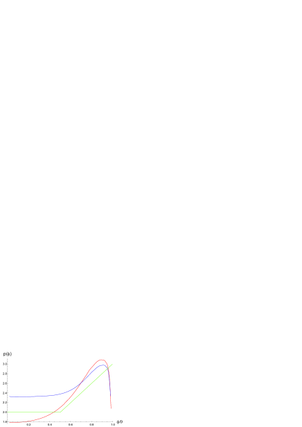
Figure 2: The function $p(\phi)$, which results in a best fit between Eq.(19) and numerically obtained tangential velocity. Here x-axis corresponds to $\phi/\theta$, where $\theta=50^{\circ}$ is the droplet contact angle. Red curve corresponds to the ethanol droplet, blue curve corresponds to the hexanol droplet. Using the shown values of $p(\phi)$, the numerical plots of $u_{\tau}(n)$ for each $\phi$ are visually indistinguishable from their best fit with Eq. (19). Green curve shows the plot of Eq. (34).

Table 1 shows the parameter values that were used in the calculations. The fluid and vapor properties were taken from [18]. Table 2 shows the contact angle, contact line radius and fitting parameters corresponding to Eq. (4) for the 25 droplets. For each droplet, we have $c=T_{0}/\Delta T-1$, and the value of $a$ is obtained with the least squares fit for a given values of $b$ and $c$. The parameter $b$ is an integer which is chosen to give the minimal value of the numerically obtained integral

$$\int_{0}^{1}\left(\frac{T(\tilde{r})}{\Delta T}-(a\tilde{r}^{b}+(1-a)\tilde{r}^{2}+c)\right)^{2}d\tilde{r},$$ (33)

where the surface temperature distribution of the drop $T(\tilde{r})$ is obtained numerically under the time independent conditions. The boundary conditions for the stationary equation $\Delta T=0$, which is numerically solved inside the drop, take the form $\partial T/\partial r=0$ for $r=0$; $T=T_{0}$ for $z=0$; ${\partial T}/{\partial n}=-LJ_{s}(r)/k$ at the drop surface. Here $\mathbf{n}$ is a normal vector to the drop surface, $J_{s}$ is determined by (2), other notations are explained in Table 1. The results in Table 2 are obtained using the boundary condition $T=T_{0}$ for $z=0$, which assumes high thermal conductivity of the substrate. High thermal conductivity of the substrate, generally, results in a single-vortex fluid flow in the droplet, while other convective regimes are also known, where the thermal conduction inside the substrate is important and should be taken into account [31, 32, 33, 34].

The numerical results show that the power exponent $p(\phi)$ in Eq. (19) is, generally, between $1.5$ and $3.5$. Some of such numerical results for $p(\phi)$ are shown in Fig. 2. The numerically obtained tangential velocities $u_{\tau}(n,\phi)$ are best fitted with Eq. (19) with the power exponents shown in Fig. 2, where the red curve corresponds to the ethanol droplet and the blue curve corresponds to the hexanol droplet. Using these values of $p(\phi)$, the numerical plots of $u_{\tau}(n)$ for each $\phi$ are visually indistinguishable from their best fit with Eq. (19). Thus, using Eq. (19) with $p(\phi)$ between $1.5$ and $3.5$ gives reasonably accurate description of $u_{\tau}(n)$ even for relatively complex single-vortex fluid flows.

Taking the trail function $p(\phi)=2$ already allows to achieve a reasonable accuracy in describing the velocity field in various droplets. In order to choose the trial function closer to its actual behavior, such as shown in Fig. 2, we have specified the trial function $p(\phi)$ to take the form

$$p(\phi)=\left\{\begin{aligned} 2&,\mbox{\qquad for\quad}\phi/\theta\leq 1/2,\\ 2+{4\delta}/{\pi}\left(1-\cos\left({\pi}\left({\phi}/{\theta}-1/2\right)/{(2\delta)}\right)\right)&,\mbox{\qquad for\quad}1/2<\phi/\theta\leq 1/2+\delta,\\ 1+2{\phi}/{\theta}-2(1-2/\pi)\delta&,\mbox{\qquad for\quad}\phi/\theta>1/2+\delta,\end{aligned}\right.$$ (34)

where $\delta=10^{-2}$. Plot of Eq. (34) is shown as a green curve in Fig. 2. This function is equal to $2$ for $\phi\leq\theta/2$, it smoothly changes from $2$ to $3$ when $\phi$ changes from $\theta/2$ to $\theta$ and its derivative is continuous. We note that the function $p(\phi)$ does not depend on the contact angle or the liquid properties.

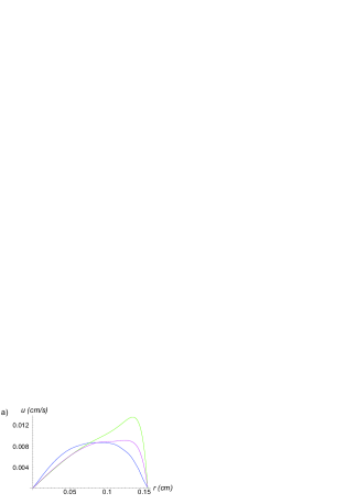
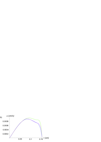
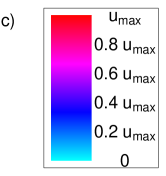
Figure 3: The surface velocity (cm/s) vs $r$ (cm) for the hexanol droplet with a) $\theta=50^{\circ}$ and b) $\theta=20^{\circ}$. Blue curve is the numerically obtained surface velocity. Green curve: the surface velocity in the heuristic extension of the lubrication approximation. Purple curve: the surface velocity in the $n\tau$-description derived in Sec. 3. Right panel: color scale for Figs. 4 and 6, where the values $u_{max}$ are given in Table 3.

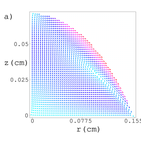
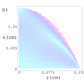
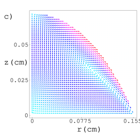
Figure 4: Vector field plots of the velocity field containing single vortex for the hexanol droplet with $\theta=50^{\circ}$: numerically obtained velocity field, the velocity field in the heuristic extension of the lubrication approximation and in the $n\tau$-description.

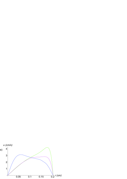
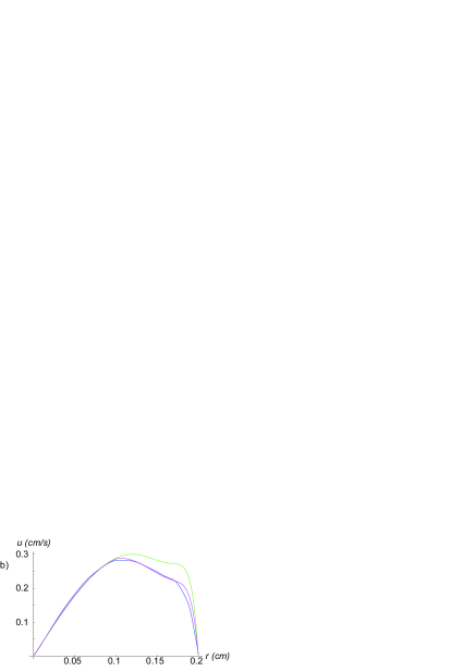
Figure 5: The surface velocity (cm/s) vs $r$ (cm) for the toluene droplet. Left panel: $\theta=50^{\circ}$, right panel: $\theta=20^{\circ}$. Blue curve is the numerically obtained surface velocity, which shows the “bottleneck effect” arising in the numerical results only when the Marangoni number exceeds 3000. Green curve: the surface velocity in the heuristic extension of the lubrication approximation. Purple curve: the surface velocity in the $n\tau$-description derived in Sec. 3.

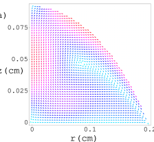
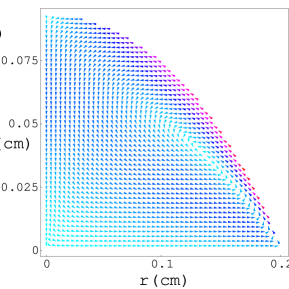
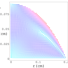
Figure 6: Vector field plots of the velocity field containing single vortex for the toluene droplet with $\theta=50^{\circ}$: numerically obtained velocity field, which shows the “bottleneck effect” arising in the numerical results only when the Marangoni number exceeds 3000, the velocity field in the heuristic extension of the lubrication approximation and in the $n\tau$-description.

The numerical simulation for the fluid flows was carried out with the method described in [13], where the droplet surface was considered to be fixed, the surface temperature was taken in accordance with Table 2 and Eq. (4), and the heat convection was switched off. Although the inverse Stanton number for many of the considered droplets is quite large, we switch off the heat convection, since all the three approaches obviously do not take into account such effects. Among the droplets considered, the inverse Stanton number is sufficiently small for a hexanol droplet with a contact angle $20^{\circ}$. It will also be small for droplets of a smaller size. During the numerical calculation, the array of velocity values is obtained from the stream function [13] using the relations

$$v_{r}(i,j)=\frac{\psi_{i,j+1}-\psi_{i,j}}{ih_{x}h_{y}},\qquad\qquad v_{z}(i,j)=\frac{\psi_{i,j}-\psi_{i+1,j}}{(i+1/2)h_{x}h_{x}}.$$ (35)

Therefore, we will estimate the deviation of the numerical velocity field from the analytically obtained velocity field using the following mean-square deviations:

$$\sigma_{r} = \frac{1}{N}\sqrt{\sum_{i,j=0}^{N-1}\left(v_{r}(i,j)-u_{r}\left(ih_{x},\left(j+1/2\right)h_{y}\right)\right)^{2}},$$ (36)

$$\sigma_{z} = \frac{1}{N}\sqrt{\sum_{i,j=0}^{N-1}\left(v_{z}(i,j)-u_{z}\left(\left(i+1/2\right)h_{x},jh_{y}\right)\right)^{2}}.$$ (37)

Here $N=200$ is the mesh size, $h_{x}=R/N$, $h_{y}=h/N$. One more characteristic value of the velocity field is $u_{max}$, the absolute value of maximal velocity at the surface of the droplet. Tables 3 and 4 show $u_{max}$ obtained with numerical simulation, with heuristic extension of the lubrication approximation, and with the two versions of the $n\tau$-approximation which employ $p(\phi)=2$ and $p(\phi)$ taken from Eq. (34) correspondingly. The tables also show the values of $\sigma_{r}$ and $\sigma_{z}$ for the analytical descriptions. Table 4 contains the results for the droplet of 2-propanol, where the size of the droplet is varied. Also, table 4 contains the comparison of analytical and numerical results for the droplet of virtual liquid with variable viscosity, where all other characteristics coincide with those of 2-propanol.

Table 3 and Figs. 3b and 5b show for the case $\theta<30^{\circ}$, when the droplets are relatively flat, that all the three approximate analytical descriptions, including the lubrication approximation, agree well with the numerically obtained velocity field, though the $n\tau$-approach with Eq. (34) is the most precise.

For large contact angles, Table 3 shows that the accuracy of the $n\tau$-description exceeds that of the heuristic extension of lubrication approximation by a factor of about $1.5$, and also the $n\tau$-description results in a much more precise value of the maximal surface velocity $u_{max}$. The heuristic extension of the lubrication approximation still works within $15$–$30$ per cent for droplets with large contact angles, where the assumptions a), b) and c) of Sec 2 are not justified.

The droplets under consideration have a wide spread of values of the Marangoni number $\tilde{\mathrm{M_{a}}}=-\sigma^{\prime}_{T}c_{V}\Delta T\rho h/(\eta k)$, starting from $10$ for the droplet of 1-hexanol, up to $3450$ for the toluene droplet. For droplets of toluene, propanol, octane and ethanol, the droplet size is much smaller than the Marangoni cell size [25, 13] on the flat fluid film containing the same liquid of the same height, while for droplets of butanol and hexanol, the droplet size and the Marangoni cell size are of the same order.

The comparison shows that the discrepancy between the numerical results and the analytical descriptions is considerably large only for droplets with huge Marangoni numbers and, therefore, large contact angles. Numerical results show that when the Marangoni number exceeds $3000$, the “bottleneck effect” will take place. This means that the vortex center becomes sufficiently close to the symmetry axis due to large Marangoni forces. This results in substantial increase of downward velocities along the symmetry axis. This is shown in Figs. 5a and 6a, where the color scale for vector field plots is shown in Fig. 3c and the values $u_{max}$ are given in Table 3. Evidently, such an effect cannot be quantitatively described without employing the Navier–Stokes equations and without taking into account the convective heat transfer. Also, it seems very probable that for such huge Marangoni numbers, Marangoni forces would rather destroy the axial symmetry of the droplet, which would result in a more complicated three-dimensional velocity field. We observed the “bottleneck effect” only for the large droplet of toluene and for the large droplet of virtual liquid with viscosity in $4$ or $8$ times smaller than that of 2-propanol (see the fourth and fifth rows in Table 4). For other droplets there is no “bottleneck effect”. For example, Figs. 3 and 4 show the velocity field for the droplet of 1-hexanol. The velocity fields for all other droplets with contact angles $50^{\circ}$ and $20^{\circ}$ are very similar to those shown in Figs. 3 and 4. Thus, the numerical results for axially symmetrical velocity field demonstrate a large discrepancy with the analytical description only when the Marangoni and the inverse Stanton number are sufficiently large, while the results are applicable when ${\mathrm{St}}^{-1}\ll 1$.

5 Conclusion

A comparatively simple and detailed description of the single vortex fluid flows, which ensures a good accuracy when the inverse Stanton number is much smaller than unity, has been developed for an axially symmetrical evaporating sessile drops of capillary size. The results have been tested and compared with the data of numerical simulations for droplets of various liquids and for a wide range of contact angles. The approach analytically addresses the boundary conditions and the mass balance equations making a simple assumption regarding tangential velocity field, without explicitly solving the Navier–Stokes equations. The results obtained signify that the boundary conditions and the mass balance equations dominate in the formation of the single vortex convection inside the droplet.

The author thanks R.G. Larson and Wei Chen for useful discussions. The simulations were partially carried out using facilities of the Supercomputing Center of Lomonosov Moscow State University [36]. The results in Secs. 3, 4 were supported by the Russian Science Foundation project No. 14-21-00158.

Table 1: The parameter values used in the calculations.

				toluene	ethanol	2-propanol	octane	1-butanol	1-hexanol
Droplet	Initial temperature	$T_{0}$	K	$293.15$	$293.15$	$293.15$	$293.15$	$293.15$	$293.15$
	Contact line radius	$R$	cm	$0.2$	$0.154$	$0.168$	$0.175$	$0.157$	$0.155$
Fluid	Density	$\rho$	g/cm3	$0.87$	$0.789$	$0.786$	$0.703$	$0.8098$	$0.8136$
	Molar mass	$\mu$	g/mole	$92.14$	$46.07$	$60.1$	$114.23$	$74.122$	$102.17$
	Thermal conductivity	$k$	W/(cm$\cdot$ K)	$1.311\cdot 10^{-3}$	$1.69\cdot 10^{-3}$	$1.35\cdot 10^{-3}$	$1.28\cdot 10^{-3}$	$1.54\cdot 10^{-3}$	$1.50\cdot 10^{-3}$
	Heat capacity	$c_{p}$	J/(mole K)	$156.7$	$112.3$	$156.5$	$254.6$	$177.2$	$240.4$
	Isochoric heat capacity	$c_{v}$	J/(g K)	$1.286$	$1.787$	$1.931$	$1.791$	$1.83$	$1.889$
	Thermal diffusivity	$\kappa$	cm2/s	$8.86\cdot 10^{-4}$	$8.79\cdot 10^{-4}$	$6.60\cdot 10^{-4}$	$8.17\cdot 10^{-4}$	$7.95\cdot 10^{-4}$	$7.84\cdot 10^{-4}$
	Dynamic viscosity	$\eta$	g/(cm$\cdot$ s)	$5.6\cdot 10^{-3}$	$1.074\cdot 10^{-2}$	$2.038\cdot 10^{-2}$	$5.08\cdot 10^{-3}$	$2.544\cdot 10^{-2}$	$4.578\cdot 10^{-2}$
	Surface tension	$\sigma$	g/s2	$28.3049$	$21.97$	$20.93$	$21.14$	$24.93$	$25.81$
	$-\partial($surface tension$)/\partial T$	$-\sigma^{\prime}_{T}$	g/(s${}^{2}\cdot$ K)	$0.1189$	$0.0832$	$0.0788$	$0.095$	$0.0898$	$0.08$
	Latent heat of evap.	$L$	J/g	$300.0$	$918.6$	$755.2$	$363.2$	$706.27$	$603.0$
Vapor	Diffusion constant	$D$	cm2/s	$0.1449$	$0.1181$	$0.1013$	$0.0616$	$0.0861$	$0.0621$
	Saturated vapor density	$u_{s}$	g/cm3	$1.27\cdot 10^{-4}$	$1.46\cdot 10^{-4}$	$1.38\cdot 10^{-4}$	$8.57\cdot 10^{-5}$	$2.76\cdot 10^{-5}$	$6.55\cdot 10^{-6}$
	Local evap. rate at apex	$J_{0}$	g/(cm${}^{2}\cdot$ s)	$9.2\cdot 10^{-5}$	$1.12\cdot 10^{-4}$	$8.2\cdot 10^{-5}$	$2.9\cdot 10^{-5}$	$1.55\cdot 10^{-5}$	$2.7\cdot 10^{-6}$

Table 2: Fitting parameters for calculation of surface temperature.

	$\theta$	$R$, cm	$\Delta T$, K	a	b	c
1-butanol	$50^{\circ}$	0.157	0.529506	0.3793	10	552.629
1-butanol	$20^{\circ}$	0.157	0.154023	0.324516	15	1902.29
ethanol	$50^{\circ}$	0.154	4.55357	0.379299	10	63.3781
ethanol	$20^{\circ}$	0.154	1.32454	0.324514	15	220.321
octane	$50^{\circ}$	0.175	0.727793	0.379299	10	401.793
octane	$20^{\circ}$	0.175	0.2117	0.324512	15	1383.74
2-propanol	$50^{\circ}$	0.168	3.7995	0.379299	10	76.1549
2-propanol	$20^{\circ}$	0.168	1.1052	0.324514	15	264.246
toluene	$50^{\circ}$	0.2	2.04597	0.379299	10	142.281
toluene	$20^{\circ}$	0.2	0.595135	0.324515	15	491.577
1-hexanol	$10^{\circ}$	0.155	0.010597	0.29475	24	27662.5
1-hexanol	$15^{\circ}$	0.155	0.016353	0.337253	16	17925.4
1-hexanol	$20^{\circ}$	0.155	0.023109	0.324521	15	12684.5
1-hexanol	$25^{\circ}$	0.155	0.030568	0.317682	14	9589.09
1-hexanol	$30^{\circ}$	0.155	0.038757	0.317114	13	7562.79
1-hexanol	$35^{\circ}$	0.155	0.047704	0.323616	12	6144.19
1-hexanol	$40^{\circ}$	0.155	0.057442	0.337952	11	5102.41
1-hexanol	$45^{\circ}$	0.155	0.068007	0.3489	11	4309.59
1-hexanol	$50^{\circ}$	0.155	0.079445	0.379306	10	3688.97
1-hexanol	$55^{\circ}$	0.155	0.091807	0.403695	10	3192.11
1-hexanol	$60^{\circ}$	0.155	0.105159	0.434731	10	2786.68
2-propanol	$50^{\circ}$	0.1	3.7995	0.379299	10	76.1549
2-propanol	$50^{\circ}$	0.05	3.7995	0.379299	10	76.1549
2-propanol	$50^{\circ}$	0.02	3.7995	0.379299	10	76.1549
2-propanol	$50^{\circ}$	0.01	3.7995	0.379299	10	76.1549

Table 3: Accuracy of the analytical descriptions. The values of $u_{max}$, $\sigma_{r}$ and $\sigma_{z}$ are in cm/s.

	$\theta$	Numerical	Lubrication	$n\tau$, $p=2$	$n\tau$, (34)	Lubrication		$n\tau$, $p=2$		$n\tau$, (34)
		$u_{max}$	$u_{max}$	$u_{max}$	$u_{max}$	$\sigma_{r}$	$\sigma_{z}$	$\sigma_{r}$	$\sigma_{z}$	$\sigma_{r}$	$\sigma_{z}$
1-butanol	$50^{\circ}$	0.12	0.18	0.14	0.122	0.0098	0.0064	0.0092	0.0054	0.0077	0.0047
1-butanol	$20^{\circ}$	0.0123	0.0129	0.0127	0.0124	$8.7\cdot 10^{-4}$	$1.9\cdot 10^{-4}$	$8.5\cdot 10^{-4}$	$1.9\cdot 10^{-4}$	$8.3\cdot 10^{-4}$	$1.8\cdot 10^{-4}$
ethanol	$50^{\circ}$	2.29	3.43	2.64	2.31	0.221	0.189	0.187	0.135	0.160	0.122
ethanol	$20^{\circ}$	0.232	0.244	0.240	0.234	0.017	0.0037	0.0162	0.0036	0.016	0.0034
octane	$50^{\circ}$	0.876	1.324	1.017	0.889	0.0812	0.065	0.070	0.046	0.059	0.040
octane	$20^{\circ}$	0.089	0.094	0.093	0.090	0.0064	0.0014	0.0063	0.0014	0.0061	0.0013
2-propanol	$50^{\circ}$	0.929	1.429	1.098	0.960	0.078	0.053	0.0716	0.0409	0.060	0.035
2-propanol	$20^{\circ}$	0.097	0.101	0.100	0.098	0.0069	0.0015	0.0068	0.0015	0.0066	0.0014
toluene	$50^{\circ}$	3.14	4.23	3.25	2.84	0.49	0.62	0.43	0.55	0.41	0.54
toluene	$20^{\circ}$	0.285	0.300	0.295	0.288	0.020	0.0046	0.020	0.0044	0.019	0.0042
1-hexanol	$10^{\circ}$	$2.2\cdot 10^{-4}$	$2.2\cdot 10^{-4}$	$2.2\cdot 10^{-4}$	$2.2\cdot 10^{-4}$	$1.5\cdot 10^{-5}$	$1.5\cdot 10^{-6}$	$1.5\cdot 10^{-5}$	$1.5\cdot 10^{-6}$	$1.4\cdot 10^{-5}$	$1.5\cdot 10^{-6}$
1-hexanol	$15^{\circ}$	$4.7\cdot 10^{-4}$	$4.9\cdot 10^{-4}$	$4.8\cdot 10^{-4}$	$4.7\cdot 10^{-4}$	$3.4\cdot 10^{-5}$	$5.5\cdot 10^{-6}$	$3.4\cdot 10^{-5}$	$5.4\cdot 10^{-6}$	$3.3\cdot 10^{-5}$	$5.2\cdot 10^{-6}$
1-hexanol	$20^{\circ}$	$9.1\cdot 10^{-4}$	$9.6\cdot 10^{-4}$	$9.4\cdot 10^{-4}$	$9.2\cdot 10^{-4}$	$6.5\cdot 10^{-5}$	$1.4\cdot 10^{-5}$	$6.4\cdot 10^{-5}$	$1.4\cdot 10^{-5}$	$6.2\cdot 10^{-5}$	$1.3\cdot 10^{-5}$
1-hexanol	$25^{\circ}$	$1.54\cdot 10^{-3}$	$1.64\cdot 10^{-3}$	$1.6\cdot 10^{-3}$	$1.57\cdot 10^{-3}$	$1.1\cdot 10^{-4}$	$3.1\cdot 10^{-5}$	$1.1\cdot 10^{-4}$	$3.0\cdot 10^{-5}$	$1.1\cdot 10^{-4}$	$2.9\cdot 10^{-5}$
1-hexanol	$30^{\circ}$	$2.4\cdot 10^{-3}$	$2.6\cdot 10^{-3}$	$2.5\cdot 10^{-3}$	$2.4\cdot 10^{-3}$	$1.8\cdot 10^{-4}$	$6.0\cdot 10^{-5}$	$1.7\cdot 10^{-4}$	$5.6\cdot 10^{-5}$	$1.6\cdot 10^{-4}$	$5.3\cdot 10^{-5}$
1-hexanol	$35^{\circ}$	$3.5\cdot 10^{-3}$	$4.0\cdot 10^{-3}$	$3.7\cdot 10^{-3}$	$3.6\cdot 10^{-3}$	$2.6\cdot 10^{-4}$	$1.1\cdot 10^{-4}$	$2.5\cdot 10^{-4}$	$9.8\cdot 10^{-5}$	$2.3\cdot 10^{-4}$	$9.2\cdot 10^{-5}$
1-hexanol	$40^{\circ}$	$4.8\cdot 10^{-3}$	$6.2\cdot 10^{-3}$	$5.3\cdot 10^{-3}$	$4.9\cdot 10^{-3}$	$3.8\cdot 10^{-4}$	$1.8\cdot 10^{-4}$	$3.6\cdot 10^{-4}$	$1.6\cdot 10^{-4}$	$3.3\cdot 10^{-4}$	$1.5\cdot 10^{-4}$
1-hexanol	$45^{\circ}$	$6.5\cdot 10^{-3}$	$9.0\cdot 10^{-3}$	$7.3\cdot 10^{-3}$	$6.7\cdot 10^{-3}$	$5.2\cdot 10^{-4}$	$2.9\cdot 10^{-4}$	$4.9\cdot 10^{-4}$	$2.5\cdot 10^{-4}$	$4.3\cdot 10^{-4}$	$2.3\cdot 10^{-4}$
1-hexanol	$50^{\circ}$	$8.73\cdot 10^{-3}$	$1.35\cdot 10^{-2}$	$1.0\cdot 10^{-2}$	$9.07\cdot 10^{-3}$	$7.3\cdot 10^{-4}$	$4.7\cdot 10^{-4}$	$6.9\cdot 10^{-4}$	$4.0\cdot 10^{-4}$	$5.8\cdot 10^{-4}$	$3.5\cdot 10^{-4}$
1-hexanol	$55^{\circ}$	$1.1\cdot 10^{-2}$	$2.0\cdot 10^{-2}$	$1.4\cdot 10^{-2}$	$1.2\cdot 10^{-2}$	$9.8\cdot 10^{-4}$	$7.4\cdot 10^{-4}$	$9.6\cdot 10^{-4}$	$6.2\cdot 10^{-4}$	$7.5\cdot 10^{-4}$	$5.2\cdot 10^{-4}$
1-hexanol	$60^{\circ}$	$1.5\cdot 10^{-2}$	$2.9\cdot 10^{-2}$	$1.9\cdot 10^{-2}$	$1.7\cdot 10^{-2}$	$1.3\cdot 10^{-3}$	$1.1\cdot 10^{-3}$	$1.4\cdot 10^{-3}$	$9.5\cdot 10^{-4}$	$1.0\cdot 10^{-3}$	$7.7\cdot 10^{-4}$

Table 4: Accuracy of the analytical descriptions. Dependence on the viscosity and on the contact line radius. The values of $u_{max}$, $\sigma_{r}$ and $\sigma_{z}$ are in cm/s.

	$\theta$	$R$, cm	$\eta/\eta_{0}$	Numerical	Lubrication	$n\tau$, $p=2$	$n\tau$, (34)	Lubrication		$n\tau$, $p=2$		$n\tau$, (34)
				$u_{max}$	$u_{max}$	$u_{max}$	$u_{max}$	$\sigma_{r}$	$\sigma_{z}$	$\sigma_{r}$	$\sigma_{z}$	$\sigma_{r}$	$\sigma_{z}$
2-propanol	$50^{\circ}$	0.168	2	0.46	0.71	0.55	0.48	0.039	0.025	0.036	0.021	0.030	0.018
2-propanol	$50^{\circ}$	0.168	1	0.929	1.429	1.098	0.960	0.078	0.053	0.072	0.041	0.060	0.035
2-propanol	$50^{\circ}$	0.168	0.5	1.90	2.86	2.20	1.92	0.182	0.153	0.154	0.109	0.131	0.097
2-propanol	$50^{\circ}$	0.168	0.25	4.31	5.72	4.39	3.84	0.70	0.90	0.622	0.807	0.59	0.79
2-propanol	$50^{\circ}$	0.168	0.125	8.23	11.43	8.78	7.68	1.70	2.35	1.567	2.190	1.49	2.16
2-propanol	$50^{\circ}$	0.1	1	0.93	1.43	1.098	0.96	0.078	0.052	0.072	0.041	0.060	0.035
2-propanol	$50^{\circ}$	0.05	1	0.92	1.43	1.098	0.96	0.077	0.051	0.072	0.042	0.060	0.036
2-propanol	$50^{\circ}$	0.02	1	0.92	1.43	1.098	0.96	0.077	0.050	0.072	0.042	0.061	0.037
2-propanol	$50^{\circ}$	0.01	1	0.92	1.42	1.098	0.96	0.077	0.050	0.072	0.043	0.061	0.037

References

- [1]
- [2] J. C. Maxwell, “Diffusion”- Collected Scientific Papers, Cambridge: Encyclopedia Britannica, 1877.
- [3] I. Langmuir, The evaporation of small spheres, Phys. Rev. 12, No. 5, pp. 368–370 (1918).
- [4] N. A. Fuchs, Evaporation and droplet growth in gaseous media (Pergamon Press, Oxford, 1959).
- [5] H.Y. Erbil, Evaporation of pure liquid sessile and spherical suspended drops: A review, Adv. Colloid Int. Sci. 170, 67 (2012).
- [6] R.G. Larson, Transport and deposition patterns in drying sessile droplets, AIChE Journal 60(5), 1538 (2014).
- [7] H. Hu, R.G. Larson, Marangoni effect reverses coffee-ring depositions, J. Phys. Chem. B 110, 7090 (2006).
- [8] R. Savino, S. Fico, Transient Marangoni convection in hanging evaporating drops, Phys. Fluids 16, 3738 (2004).
- [9] A.K. Thokchom, S.K. Majumder, A. Singh, Internal fluid motion and particle transport in externally heated sessile droplets, AIChE Journal, 62(4), 1308 (2016).
- [10] H. Masoud, J. D. Felske, Analytical solution for inviscid flow inside an evaporating sessile drop, Phys. Rev. E 79, 016301 (2009).
- [11] Yu. Yu. Tarasevich, Simple analytical model of capillary flow in an evaporating sessile drop, Phys. Rev. E 71, 027301 (2005).
- [12] H. Gelderblom et.al., How water droplets evaporate on a superhydrophobic substrate, Phys. Rev. E 83, 026306 (2011).
- [13] L.Yu. Barash, T.P. Bigioni, V.M. Vinokur, L.N. Shchur, Evaporation and fluid dynamics of a sessile drop of capillary size, Phys. Rev. E 79, 046301 (2009).
- [14] H. Hu, R. G. Larson, Analysis of the Effects of Marangoni Stresses on the Microflow in an Evaporating Sessile Droplet, Langmuir 21, 3972 (2005).
- [15] H. Hu, R. G. Larson, Analysis of the Microfluid Flow in an Evaporating Sessile Droplet, Langmuir 21, 3963 (2005).
- [16] R. D. Deegan et al., Contact line deposits in an evaporating drop, Phys. Rev. E 62, 756 (2000).
- [17] H. Hu, R. G. Larson, Evaporation of a Sessile Droplet on a Substrate, J. Phys. Chem. B 106, 1334 (2002).
- [18] D. R. Lide, CRC Handbook of Chemistry and Physics (CRC Press, 2004).
- [19] P. G. de Gennes, Wetting: statics and dynamics, Rev. Mod. Phys. 57, 827 (1985).
- [20] D. Bonn, J. Eggers, J. Indekeu, J. Meunier, E. Rolley, Wetting and spreading, Rev. Mod. Phys. 81, 739 (2009).
- [21] C. Huh and L. E. Scriven, Hydrodynamic model of steady movement of a solid/liquid/fluid contact line, J. Colloid Interface Sci. 35, 85 (1971).
- [22] A. J. Petsi, V. N. Burganos, Stokes flow inside an evaporating liquid line for any contact angle, Phys. Rev. E 78, 036324 (2008).
- [23] A. Rednikov and P. Colinet, Singularity-free description of moving contact lines for volatile liquids, Phys. Rev. E 87, 010401(R) (2013).
-
[24]
A. Rednikov,
Relaxation of contact-line singularities solely by the Kelvin effect
and apparent contact angles for isothermal volatile liquids in contact with air,
http://meetings.aps.org/Meeting/DFD13/Session/G33.7 - [25] J. R. A. Pearson, On convection cells induced by surface tension, J. Fluid Mech. 4, 489 (1958).
- [26] F. Duan, V. K. Badam, F. Durst, C. A. Ward, Thermocapillary transport of energy during water evaporation, Phys. Rev. E 72, 056303 (2005).
- [27] N. Murisic and L. Kondic, On evaporation of sessile drops with moving contact lines, J. Fluid Mech. 679, 219 (2011).
- [28] B. Sobac, D. Brutin, Thermocapillary instabilities in an evaporating drop deposited onto a heated substrate, Phys. Fluids, 24, 032103 (2012)
- [29] F. Carle, B. Sobac, D. Brutin, Experimental evidence of the atmospheric convective transport contribution to sessile droplet evaporation, Appl. Phys. Lett. 102, 061603 (2013).
- [30] F. Girard, M. Antoni, K. Sefiane, Use of IR thermography to investigate heated droplet evaporation and contact line dynamics, Langmuir 27, 6744 (2011)
- [31] W. D. Ristenpart, P. G. Kim, C. Domingues, J. Wan, H. A. Stone, Phys. Rev. Lett. 99, 234502 (2007).
-
[32]
L.Yu. Barash,
Dependence of the fluid convection in an evaporating sessile droplet on the thermal
conductivity of the substrate,
http://ccp2011.ornl.gov/pdf/Abstracts/Barash_Lev_9.1b_8.pdf - [33] L.Yu. Barash, Dependence of fluid flows in an evaporating sessile droplet on the characteristics of the substrate, Int. J. Heat and Mass Transfer 84, 419 (2015)
- [34] K. Zhang, L. Ma, X. Xu, L. Luo, D. Guo, Temperature distribution along the surface of evaporating droplets, Phys. Rev. E 89, 032404 (2014).
- [35] S. Semenov, V.M. Starov, R.G. Rubio, M.G. Velarde, Computer simulations of evaporation of pinned sessile droplets: influence of kinetic effects, Langmuir 28, 15203 (2012)
- [36] Voevodin Vl.V., Zhumatiy S.A., Sobolev S.I., Antonov A.S., Bryzgalov P.A., Nikitenko D.A., Stefanov K.S., Voevodin Vad.V., Practice of ”Lomonosov” Supercomputer, Open Systems J., Moscow: Open Systems Publ., 2012, no.7. (In Russian)