Implications of Plasma Beam Instabilities for the Statistics of the Fermi Hard Gamma-ray Blazars and the Origin of the Extragalactic Gamma-Ray Background

Abstract

Fermi has been instrumental in constraining the luminosity function and redshift evolution of gamma-ray bright blazars. This includes limits upon the spectrum and anisotropy of the extragalactic gamma-ray background (EGRB), redshift distribution of nearby Fermi active galactic nuclei (AGN), and the construction of a $\log\mathcal{N}$-$\log S$ relation. Based upon these, it has been argued that the evolution of the gamma-ray bright blazar population must be much less dramatic than that of other AGN. However, critical to such claims is the assumption that inverse Compton cascades reprocess emission above a TeV into the Fermi energy range, substantially enhancing the strength of the observed limits. Here we demonstrate that in the absence of such a process, due, e.g., to the presence of virulent plasma beam instabilities that preempt the cascade, a population of TeV-bright blazars that evolve similarly to quasars is consistent with the population of hard gamma-ray blazars observed by Fermi. Specifically, we show that a simple model for the properties and luminosity function is simultaneously able to reproduce their $\log\mathcal{N}$-$\log S$ relation, local redshift distribution, and contribution to the EGRB and its anisotropy without any free parameters. Insofar the naturalness of a picture in which the hard gamma-ray blazar population exhibits the strong redshift evolution observed in other tracers of the cosmological history of accretion onto halos is desirable, this lends support for the absence of the inverse Compton cascades and the existence of the beam plasma instabilities.

1 Introduction

1.1 Blazars in the Fermi era

The Large Area Telescope (LAT) onboard the Fermi gamma-ray space telescope has become a powerful tool for studying gamma-ray bright active galactic nuclei (AGNs), placing the most stringent constraints to date upon their numbers and evolution. In practice, this is performed via a variety of methods, including the flux and redshift distributions of nearby sources, and the extragalactic gamma-ray background (EGRB) due to unresolved sources at high redshift. Each of these effectively probes different projections of the evolving luminosity function of the gamma-ray bright objects, and thus taken together provides considerable traction upon their populations at low and high redshifts.

The Fermi AGN sample is overwhelmingly dominated by blazars, with a handful of radio and starburst galaxies comprising the remainder (see, e.g., Table 5 of Ackermann et al., 2011). The population of blazars is itself often sub-divided into a number of sub-categories, depending primarily upon their optical properties. The most populated are the flat-spectrum radio sources (FSRQs) and BL Lacs, both of which are further segregated into low, intermediate, and high synchrotron peak sources (LSP, ISP, HSP, respectively). The latter categories roughly correspond to the hardness or softness of the gamma-ray spectrum, $E^{2}dN/dE$, at energies relevant for Fermi, with HSPs being harder than ISPs which are harder than LSPs. Typically, the FSRQs are considerably softer than the BL Lacs, and thus appear primarily at low energies ($\lesssim 10$ GeV). In contrast, a number of BL Lacs exhibit rising spectra between 1 GeV and 100 GeV, which we define as “hard gamma-ray blazars”.

The rising Fermi spectra of the hard gamma-ray blazars suggest a natural identification with the observed set of TeV blazars, detected and characterized by imaging atmospheric Cerenkov telescopes such as H.E.S.S., VERITAS, and MAGIC. As for Fermi, the extragalactic TeV universe is dominated by blazars: of the 28 objects with well-defined spectral energy distributions (SEDs) listed in Broderick et al. (2012), 24 are blazars, which we refer to as the “TeV blazars”. Thus, any limitation upon the evolution of the hard gamma-ray blazar population implies a corresponding constraint upon the TeV blazars, and vice versa.

The TeV blazars are all relatively nearby, with $z\sim 0.1$ typically. This is the result of the annihilation of TeV gamma-rays upon the extragalactic background light (EBL), and the subsequent generation of a relativistic population of pairs (Gould & Schréder, 1967; Salamon & Stecker, 1998; Neronov & Semikoz, 2009). Typical gamma-ray mean free paths range from 30 Mpc to 1 Gpc, depending upon gamma-ray energy and source redshift, explaining the paucity of high-redshift TeV sources. The subsequent evolution of the energetic population of pairs is subject to two competing scenarios.

Historically, it has been assumed that these cool primarily by Comptonizing the cosmic microwave background, resulting in an inverse Compton cascade that effectively reprocesses the original TeV emission to energies below 100 GeV. The assumption that this reprocessing occurs has a dramatic impact upon the implications Fermi has for the TeV blazar population. In this first scenario, stringent constraints on the number of hard gamma-ray blazars at high redshift can be derived from the EGRB, for which Fermi has provided the most precise estimate. Even based upon EGRET data, it has been well established that in the presence of inverse Compton cascades the TeV blazar population cannot exhibit the dramatic evolution that characterizes other AGN specifically, and other tracers of the cosmological history of accretion onto galactic halos more generally (e.g., star formation), with the most recent Fermi EGRB limits implying that their co-moving number density be essentially fixed (Narumoto & Totani, 2006; Kneiske & Mannheim, 2008; Inoue & Totani, 2009; Venters, 2010). This represents a substantial obstacle to unifying the hard gamma-ray blazar population with that of other AGN, is at odds with the underlying physical picture of accreting black hole systems, and suggests an unlikely conspiracy between accretion physics and the formation of structure.

In a series of papers (Broderick et al., 2012; Chang et al., 2012; Pfrommer et al., 2012, hereafter Paper I, Paper II, Paper III) and Puchwein et al. (2012), we have explored the possible impact of beam-plasma instabilities upon the gamma-ray emission of bright TeV sources and their subsequent cosmological consequences. We found that in this second scenario a variety of cosmological puzzles, most importantly the statistics of the high-redshift Ly$\alpha$ forest, were naturally resolved if the VHEGR emission from TeV blazars was dumped into heat in the intergalactic medium, as anticipated by such plasma instabilities. However, to do so requires a much more rapidly rising TeV blazar co-moving number density than implied by previous analyses of the EGRB, namely one similar to that of quasars and qualitatively consistent with these other examples that depend on the cosmological history of accretion (e.g., star formation, radio galaxies, AGNs, galactic merger rates, etc.). As shown in Paper I, the apparent tension with the above discussed constraints from the EGRB is reconciled by the lack of significant inverse Compton cascades, preempted by the plasma instabilities responsible for depositing the VHEGR luminosity into the intergalactic medium. Without the inverse Compton cascades, it is possible to quantitatively reproduce both the redshift-dependent number of hard gamma-ray blazars listed in the First Fermi LAT AGN Catalog (1LAC, Abdo et al., 2010b), and the EGRB spectrum above 10 GeV.

The recent release of the 2 Year Fermi-LAT AGN Catalog (2LAC, Ackermann et al., 2011) and the First Fermi-LAT Catalog of $>10$ GeV sources (1FHL, Ackermann et al., 2013), motivates a reevaluation of the Fermi constraints upon the evolution of the number and luminosity distribution of the hard gamma-ray blazars within the context of a considerably more complete set of resolved Fermi sources. With the luminosity function posited in Paper I, here we explicitly construct the expected flux and redshift distributions, and the Fermi EGRB, and directly assess the viability of a quasar-like evolution in the hard gamma-ray blazar population. Generally, we find excellent agreement where expected, implying that in the absence of inverse Compton cascades (preempted, e.g., by plasma instabilities) it is possible to unify the hard gamma-ray blazars with AGN generally.

1.2 Methodology and Outline

Our primary goal is to observationally probe the redshift-dependent luminosity function of the TeV blazars. In practice, this is complicated by the small number and limited redshift range of the known TeV blazars. The sample of observed TeV blazars is strongly biased in favor of nearby, X-ray selected BL Lac objects. To address those selection effects, we use the Fermi hard gamma-ray blazars (defined by an intrinsic photon spectral index $\leq 2$) as proxies.

At low redshift ($z\lesssim 0.2$), the cosmological redshift and absorption on the EBL are negligible below 100 GeV, and the two blazar populations are directly comparable. We exploit this to empirically define the distribution of intrinsic spectra relevant for the hard gamma-ray blazars, extending the luminosity function described in Paper I and removing a key degeneracy therein.

However, even at moderate redshifts ($z\gtrsim 0.2$) the absorption on the EBL substantially softens the spectra below 100 GeV (Ackermann et al., 2012c), and this must be taken into account in the source identification. Where direct comparisons to the Fermi blazar sample are made, we make the conservative choice of considering only objects with observed photon spectral indexes $\leq 2$, which necessarily implies that the intrinsic photon spectral indexes are also $\leq 2$ (Sections 3.1 and 3.3). For concreteness, we define the “hard Fermi blazars” to be those objects that exhibit a rising spectrum, with index $\Gamma_{F}\leq 2$ in the energy band 1–100 GeV, where $E^{2}dN/dE\propto E^{2-\Gamma_{F}}$. For consistency it is necessary to restrict the expected source population as well, and therefore we construct an approximate relationship between the observed and intrinsic photon spectral indexes. Where comparison with the Fermi blazar sample is not required, e.g., for modeling of the extragalactic gamma-ray background, we consider the full hard gamma-ray population, restricting only the intrinsic spectra (Section 3.4).

In Section 2 we define the TeV blazar luminosity function, describe its regime of validity, and relate it to the luminosity function of the Fermi hard gamma-ray blazars generally. In Section 3 we review the definitions of the various Fermi constraints and compare the expectations from our TeV blazar luminosity functions. Finally, discussion and conclusions are contained in Section 4.

2 The Hard Gamma-ray Blazar Luminosity Function

Here we construct a luminosity function for the hard gamma-ray blazars, beginning with a review of the luminosity function for the TeV blazars constructed in Paper I. Critical to producing an analogous luminosity function for the Fermi hard gamma-ray blazars is the relationship between the Fermi band (here 100 MeV–100 GeV) and the intrinsic isotropic equivalent TeV luminosity (100 GeV – 10 TeV).

2.1 The TeV Blazar Luminosity Function

The vast majority of extragalactic TeV sources have also been identified by Fermi, and thus there is a close relationship between the TeV blazars and the Fermi hard gamma-ray blazars (defined explicitly below).

The TeV blazars typically have falling SEDs above a TeV, with the brightest sources having a photon spectral index of $\Gamma_{\rm TeV}\simeq 3$ (where $\Gamma_{\rm TeV}$ is defined by $dN/dE\propto E^{-\Gamma_{\rm TeV}}$ from 100 GeV–10 TeV), implying a peak in the SED at energies $\lesssim 1$ TeV. Below 100 GeV these sources are among the hardest in the Fermi AGN sample, with rising SEDs, implying a peak above 100 GeV.

In principle, we define the TeV-band luminosity function of TeV blazars by

$$\tilde{\phi}_{B}(z,L_{\rm TeV})=\frac{d\mathcal{N}}{d\log_{10}L_{\rm TeV}\,d^{3}\!x}\,,$$ (1)

where $\mathcal{N}$ is the number of TeV blazars with isotropic equivalent TeV luminosities above $L_{\rm TeV}$, and in keeping with the notation in Papers I-III we denote quantities defined in terms of physical volumes by tildes (as opposed to co-moving volumes).

Measuring $\tilde{\phi}_{B}$ in practice is complicated by the large optical depth to annihilation on the EBL for gamma rays with energies above 100 GeV. The pair-production mean free path is both energy and redshift dependent, locally given by (Paper I)

$$D_{\rm pp}(E,z)=35\left(\frac{E}{1~{}{\rm TeV}}\right)^{-1}\left(\frac{1+z}{2}\right)^{-\zeta}~{}{\rm Mpc}\,,$$ (2)

where $\zeta=4.5$ for $z<1$ and $\zeta=0$ for $z\geq 1$ (Kneiske et al., 2004; Neronov & Semikoz, 2009). The redshift evolution is due to the EBL, and is sensitive primarily to the star formation history. The associated optical depth for a gamma-ray emitted at redshift $z$ and observed at an energy $E_{\rm obs}$, is then

$$\tau(E_{\rm obs},z)\equiv\int_{0}^{z}\frac{dD_{p}}{dz^{\prime}}\frac{dz^{\prime}}{D_{\rm pp}\left[E_{\rm obs}(1+z^{\prime}),z^{\prime}\right]}\,,$$ (3)

where $D_{P}\equiv\int cdt^{\prime}=\int cdz/[H(z)(1+z)]$ is the proper distance. At 1 TeV this is unity at a redshift of $z\simeq 0.14$, and TeV blazars are visible at only low redshifts, preventing a direct measurement of the evolution of $\tilde{\phi}_{B}$.

The existing collection of TeV blazars is the result of targeted observations, motivated by features in other wavebands, and is therefore subject to a number of ill-defined selection effects. Nevertheless, in Paper I we constructed an approximate luminosity function for these objects at $z\sim 0.1$. It was found that this was in excellent agreement with the quasar luminosity function, $\tilde{\phi}_{Q}$, given by Hopkins et al. (2007), and summarized in Appendix A, upon rescaling the bolometric luminosity and overall normalization:

$$\tilde{\phi}_{B}(0.1,L_{\rm TeV})\simeq 3.8\times 10^{-3}\tilde{\phi}_{Q}(0.1,1.8L_{\rm TeV})\,.$$ (4)

Included in this are a variety of uncertain corrections for various selection effects. Previously, we have attempted to estimate these by identifying the TeV blazars with the Fermi hard gamma-ray blazars. Within the context of the 2LAC we reconsider these, focusing upon the duty cycle ($\eta_{\rm duty}$) and source selection ($\eta_{\rm sel}$) corrections. There remains considerable uncertainty in the relevant source populations to compare, however. The TeV blazars are necessarily at very low redshift, suggesting that we should compare them only to the nearby Fermi hard gamma-ray blazar population. Less clear is what redshift cut to impose. At $z=0.1$, 0.15, and 0.2, there are 9, 14, and 17 TeV blazars and 16, 37, and 49 Fermi hard gamma-ray blazars with measured redshifts in the 2LAC, respectively (i.e., above the catalog’s flux limit). Noting that nearly all of the TeV blazars have now been detected by Fermi, this implies that the selection bias induced by the incomplete sky and time coverage of TeV observations requires a correction factor of 1.8 to 2.9. Furthermore, of the 277 Fermi hard gamma-ray blazars in the 2LAC, only 110 have measured redshifts. Assuming these are drawn from the same underlying population, this provides an additional correction of $2.5$. In combination, the associated selection correction ranges from 4.5 to 9.8. In Paper I, and implicitly employed in Equation (4), we assumed $\eta_{\rm sel}\times\eta_{\rm duty}=6.4$, intermediate to those inferred from the above. However, the origin of this factor is rather different: the decrease in $\eta_{\rm duty}$ to unity has been nearly exactly offset by the increase in the overall number of Fermi sources, and thus in $\eta_{\rm sel}$. Hence, the numerical factors in equation (4), as derived in Paper I, remain unchanged.

Motivated by the strong similarities with the local quasar luminosity function, we posited that this relationship held at large $z$ as well. This has received indirect circumstantial support via the observational consequences of the plasma-instability induced heating of the intergalactic medium described in Papers II, III and Puchwein et al. (2012). Of particular note is the great success in the quantitative reproduction of the high-$z$ Ly$\alpha$ forest.

2.2 Relationship to The Fermi Blazars

While relating the TeV blazars and the Fermi hard gamma-ray blazars is natural in principle, some care must be taken in practice. Difficulties arise from the uncertain relationship between the observed Fermi-band fluxes and $L_{\rm TeV}$, the annihilation of the high-energy gamma rays, and the distribution of source properties. Here we assume a specific family of SEDs for the TeV blazars, use these to define the associated Fermi observables, and discuss the inherent restrictions upon the Fermi blazar population implied by these choices.

2.2.1 Intrinsic Fermi Hard Gamma-ray Blazar SED

Relating the fluxes above a TeV and at energies relevant for Fermi ($\lesssim 100$ GeV), requires some knowledge about the intrinsic SED of the TeV blazars. As already mentioned, the SED above a TeV is slowly falling, with a photon spectral index of 3 typical (i.e., $E^{2}dN/dE\propto E^{-1}$). However, for the two brightest TeV blazars in the sky, Mkn 421 and 1ES 1959+650, the Fermi photon spectral indexes, defined from 1 GeV–100 GeV, are $\Gamma_{F}=1.77$ and 1.94, respectively (i.e., $E^{2}dN/dE\propto E^{0.2}$). This spectral shape is generic; TeV sources with spectra well characterized by Fermi below 100 GeV show a median shift between their photon spectral indexes below 100 GeV and above 1 TeV of 1.2 (see Figure 44 of Ackermann et al., 2011) and the typical $\Gamma_{F}$ for the hard gamma-ray blazars is $\sim 1.8$ (see below). Thus, it is clear empirically that a single power law is a poor model for the intrinsic SED (see, e.g., Figures 13 & 21 of Abdo et al., 2010c).

A more complicated SED is further motivated theoretically by the identification of the high-energy gamma-ray emission with the Comptonized synchrotron bump. Models of the blazar spectrum exhibit a peak near the TeV for the TeV-bright objects, suggesting that a similarly peaked SED must be considered in practice. Here, we model the intrinsic SED as a family of broken power laws:

$$\frac{dN}{dE}=f\left[\left(\frac{E}{E_{b}}\right)^{\Gamma_{l}}+\left(\frac{E}{E_{b}}\right)^{\Gamma_{h}}\right]^{-1}\,,$$ (5)

for some normalization $f$ (with units of ${\rm photons~{}GeV^{-1}~{}s^{-1}}$, and where we will set $E_{b}=1~{}{\rm TeV}$, $\Gamma_{h}\simeq\Gamma_{\rm TeV}=3$, chosen as typical values.

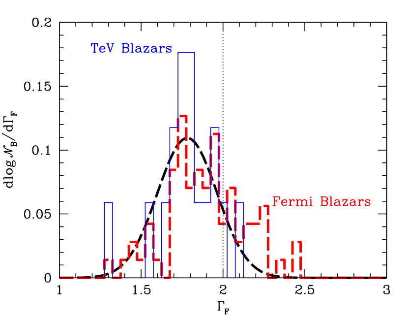
Figure 1: Distribution of the Fermi photon spectral index for TeV blazars (blue solid) and all of the Fermi blazars (red dashed) with $z<0.2$. The adopted intrinsic $\Gamma_{l}$ distribution, a Gaussian fit with mean $1.78$ and standard deviation $0.18$, is shown by a dashed line. For reference, the spectral cut defining the hard gamma-ray blazars is shown by the vertical dotted line.

The choice of $\Gamma_{l}$ is complicated by the fact that some of the observable tests described in Section 3 are sensitive to its value. However, we have some observational guidance in the form of the Fermi photon spectral indexes for the TeV blazars themselves. Figure 1 shows the $\Gamma_{F}$ distribution of the nearby TeV blazars and the Fermi hard gamma-ray blazars. The former is well fit by a Gaussian, with mean $\bar{\Gamma}_{l}=1.78$ and standard deviate $\sigma_{l}=0.18$. Based upon this we adopt the expanded luminosity function:

$$\tilde{\phi}_{B}(z,L_{\rm TeV},\Gamma_{l}) \equiv\frac{d\mathcal{N}}{d\log_{10}L_{\rm TeV}\,d^{3}\!x\,d\Gamma_{l}}$$ (6)

$$=\tilde{\phi}_{B}(z,L_{\rm TeV})\frac{e^{-(\Gamma_{l}-\bar{\Gamma}_{l})^{2}/2\sigma_{l}^{2}}}{\sqrt{2\pi}\sigma_{l}}\,.$$

Note that the $\Gamma_{F}$ distribution of the TeV blazars is somewhat harder than that of the hard gamma-ray blazars. This is likely due to the dramatic drop in TeV luminosity when the location of the Compton peak falls well below 100 GeV. We discuss this point, and the limitation it implies, in more detail in Section 2.2.3.

2.2.2 Relating the TeV blazars and the hard gamma-ray blazars

The luminosity function in Equation (6) is still presented in terms of intrinsic quantities (e.g., $\Gamma_{l}$, $L_{\rm TeV}$, etc.). However, frequently it will be necessary to relate these to quantities that are directly measurable by Fermi. These will be impacted both by the redshifting of the intrinsic spectrum and the gamma-ray annihilation on the EBL.

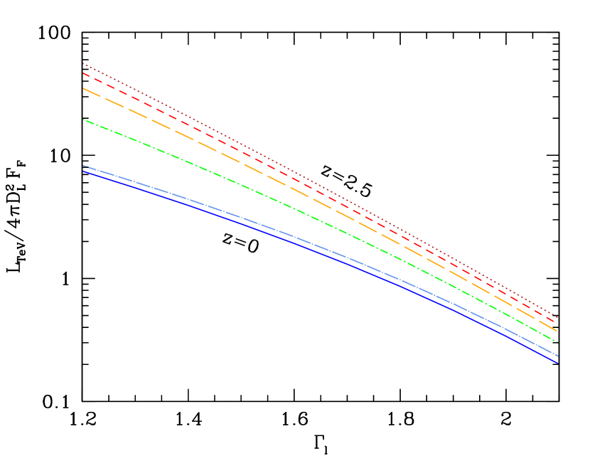
Figure 2: Ratio of the intrinsic TeV-band luminosity and the observed Fermi-band luminosity (100 MeV–100 GeV) as a function of $\Gamma_{l}$ for various redshifts, ranging from $0$ to $2.5$ in steps of $0.5$.

It is straightforward to show that the flux and fluence observed by Fermi between energies $E_{m}$ and $E_{M}$ (e.g., 100 MeV and 100 GeV) from a source at redshift $z$ is

$$F_{F}=\frac{1}{4\pi D_{L}^{2}}\int^{(1+z)E_{M}}_{(1+z)E_{m}}dE\,E\frac{dN}{dE}\,e^{-\tau[E/(1+z),z]}\,,$$ (7)

and

$$\mathcal{F}_{F}=\frac{1+z}{4\pi D_{L}^{2}}\int^{(1+z)E_{M}}_{(1+z)E_{m}}dE\,\frac{dN}{dE}\,e^{-\tau[E/(1+z),z]}\,,$$ (8)

respectively, where $D_{L}$ is the luminosity distance. Similarly, the intrinsic TeV luminosity is,

$$L_{\rm TeV}=\int_{0.1~{}{\rm TeV}}^{10~{}{\rm TeV}}dE\,E\frac{dN}{dE}\,.$$ (9)

Thus, we have a redshift and SED-dependent relationship between $F_{F}$ and $L_{\rm TeV}$:

$$\frac{L_{\rm TeV}}{4\pi D_{L}^{2}F_{F}}(z,\Gamma_{l})=\frac{\int_{0.1~{}{\rm TeV}}^{10~{}{\rm TeV}}dE\,E\,(dN/dE)}{\int^{(1+z)E_{M}}_{(1+z)E_{m}}dE\,E\,(dN/dE)\,e^{-\tau[E/(1+z),z]}}\,,$$ (10)

where the denominator is simply the isotropic equivalent Fermi-band luminosity. This is shown for a handful of redshifts as a function of $\Gamma_{l}$ in Figure 2. Note that this neglects any inverse Compton cascade component, which would otherwise increase $F_{F}$ beyond the intrinsic emission.

Similarly important for the definition of the Fermi sources is the Fermi-band photon spectral index, $\Gamma_{F}$. Again this is modified by the redshift (different portions of the intrinsic spectrum are being observed) and by absorption on the EBL. Assessing the impact these have upon the measured $\Gamma_{F}$ depends on how it is defined. Here we estimate $\Gamma_{F}$ via a least-squares fit to the redshifted and absorbed intrinsic spectrum between 1 GeV and 100 GeV, the energy range over which it is defined in the 2LAC. The impact upon $\Gamma_{F}$ is shown in Figure 3. At high redshift even intrinsically hard spectra appear soft due to absorption. For example, a source at $z=0.667$ with $\Gamma_{l}=\bar{\Gamma}_{l}=1.78$, will have a $\Gamma_{F}\simeq 2$. Thus, even moderate redshifts are sufficient to move objects out of the hard gamma-ray blazar class.

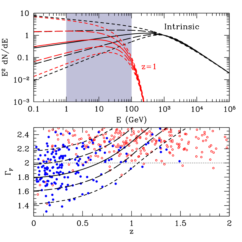
Figure 3: Top: Example intrinsic (black) and observed (red) SEDs at $z=1$ for $\Gamma_{l}=\bar{\Gamma}_{l}$ (solid), $\Gamma_{l}=\bar{\Gamma}_{l}\pm\sigma_{l}$ (long dash), and $\Gamma_{l}=\bar{\Gamma}_{l}\pm 2\sigma_{l}$ (short dash). The normalization is arbitrary, and set here so that $E^{2}dN/dE=1$ at the break energy (1 TeV). For reference the energy range over which $\Gamma_{F}$ is defined is shaded. Bottom: Inferred $\Gamma_{F}$ for the spectra in the top panel, with corresponding line types. For reference, the photon spectral index cutoff that defines the hard gamma-ray blazars is shown by the dotted line. The photon spectral indexes of the Fermi blazars are shown as a function of redshift by the points, with BL Lacs and non-BL Lacs (predominantly FSRQs) shown by the blue filled and red open circles.

Also shown in Figure 3 is the evolution of the distribution of $\Gamma_{F}$ for the Fermi blazars. This may occur for a variety of reasons, including a correlation between $\Gamma_{F}$ and bolometric luminosity (see, e.g., Ghisellini, 2011). Recently, it has been shown explicitly that this cannot account for the entirety of the spectral evolution, with absorption necessarily playing a role (Ackermann et al., 2012c). Here, we note simply that there is excellent agreement between the lower envelope of the Fermi sources and the evolution of the $\Gamma_{F}$ associated with the 2$\sigma$ lower limit upon $\Gamma_{l}$ from the TeV blazars alone (shown by the short-dash line).

2.2.3 Limitations upon the Hard Gamma-ray Blazar Luminosity Function

Our empirical TeV blazar luminosity function necessarily was constructed only for TeV-bright objects, and thus only describes the TeV-bright blazar population. As a consequence, some care must be taken in extending this to the entire Fermi blazar population. In particular, the TeV blazar luminosity function poorly constrains the population of soft gamma-ray blazars. To address this, here we restrict ourselves to the class of Fermi blazars with flat or rising spectra, and thus to the objects with intrinsic gamma-ray spectra likely to peak well above 100 GeV. That is, we consider only objects for which $\Gamma_{l}\leq 2$, for which the intrinsic SED in Equation (5) peaks around $E_{b}=1~{}{\rm TeV}$. Empirically, this is evident from the lack of TeV blazars with $\Gamma_{F}>2.1$.

Due to the spectral softening arising from absorption on the EBL and redshift, this condition upon the intrinsic SED does not translate into a unique condition upon the observed SED. That is, $\Gamma_{l}\leq 2$ does not generally imply that $\Gamma_{F}\leq 2$. The converse is, however, true: $\Gamma_{F}\leq 2$ does imply $\Gamma_{l}\leq 2$ generally, as may be seen immediately in Figure 3. Thus, where we wish to construct populations of TeV-bright objects from the Fermi blazar sample for comparison with the hard gamma-ray blazar luminosity function described in the previous section, we will consider only the Fermi hard gamma-ray blazars. This includes the $\log\mathcal{N}$-$\log S$ relation and redshift distributions described in Sections 3.1 and 3.3, respectively.

When we consider the TeV blazar contribution to the Fermi EGRB, we do not require a corresponding population of Fermi blazars, and thus retain only the more conservative condition upon $\Gamma_{l}$. Concerns regarding the generality of the associated high-energy EGRB are discussed in Section 3.4, here we simply note that the neglected population of soft gamma-ray blazars is significant only below a few GeV.

3 Comparisons with the Fermi Hard Gamma-ray Blazars

We now turn our attention to comparing the implications of the luminosity function obtained in the previous section with various measures of the Fermi hard gamma-ray population. We note that the specific properties of the luminosity function and the intrinsic spectra are now completely defined, and thus in the following comparisons to the Fermi blazar sample there are no degrees of freedom to adjust.

Both the $\log\mathcal{N}$-$\log S$ and redshift distribution probe the recent evolution of the hard gamma-ray blazar luminosity function. Since they are both one-dimensional, they are both necessarily projections of $\tilde{\phi}_{B}$. They differ in the form of the projection, measuring in different degrees the redshift evolution and the luminosity distribution of the hard gamma-ray blazars. In contrast, the Fermi isotropic EGRB is most sensitive to the unresolved sources at high redshifts, and thus probes the peak of the luminosity function in both redshift and luminosity. While all are important, the isotropic EGRB is likely to provide the most significant constraint upon the viability of rapidly evolving hard gamma-ray blazar luminosity functions.

3.1 2LAC $\log\mathcal{N}$-$\log S$ Relation

The $\log\mathcal{N}$-$\log S$ relation describes the flux distribution of a particular source class. In it, $\mathcal{N}(S)$ is simply the number of sources with fluxes $>S$, making it straightforward to define empirically. Complications arise in selecting the particular source class of interest, the definition of “flux” to be employed, and the treatment of observational selection effects. All of these are relevant for Fermi, and thus here we describe how we constructed the Fermi $\log\mathcal{N}$-$\log S$ relation for the hard gamma-ray blazars and its relation to the hard gamma-ray blazar luminosity function discussed in the previous section.

3.1.1 Observational Definition

Depending upon application, the fluence from 100 MeV–100 GeV ($\mathcal{F}_{25}$), fluence from 1 GeV–100 GeV ($\mathcal{F}_{35}$), and flux from 100 MeV–100 GeV ($F_{25}$) have all been used as “flux” measures for Fermi sources. Primarily, $\mathcal{F}_{25}$ and $F_{25}$ have been used to assess statistical properties of Fermi sources (see, e.g., Abdo et al., 2010b; Ackermann et al., 2011). This includes an empirical reconstruction of the $\log\mathcal{N}$-$\log S$ relation for the Fermi blazars in the 1LAC in terms of $\mathcal{F}_{25}$ by Singal et al. (2012). However, within the 2LAC itself, $\mathcal{F}_{35}$, is the flux measure reported.

We relate these here by assuming the spectrum across the Fermi LAT band (100 MeV to 100 GeV) is well approximated by a single power law, $dN/dE\,dt=f_{F}E^{-\Gamma_{F}}$, and therefore the fluence and flux are,

$$\mathcal{F}=f_{F}\int_{E_{m}}^{E_{M}}dEE^{-\Gamma_{F}}=\frac{f_{F}\left(E_{m}^{1-\Gamma_{F}}-E_{M}^{1-\Gamma_{F}}\right)}{\Gamma_{F}-1}\,,$$ (11)

and

$$F=f_{F}\int_{E_{m}}^{E_{M}}dEE^{1-\Gamma_{F}}=\frac{f_{F}\left(E_{m}^{2-\Gamma_{F}}-E_{M}^{2-\Gamma_{F}}\right)}{\Gamma_{F}-2}\,,$$ (12)

respectively. The normalization, $f_{F}$, is set by the reported $\mathcal{F}_{35}$, from which $\mathcal{F}_{25}$ and $F_{25}$ may then be readily computed (see the Appendix B for explicit expressions).

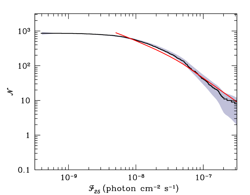
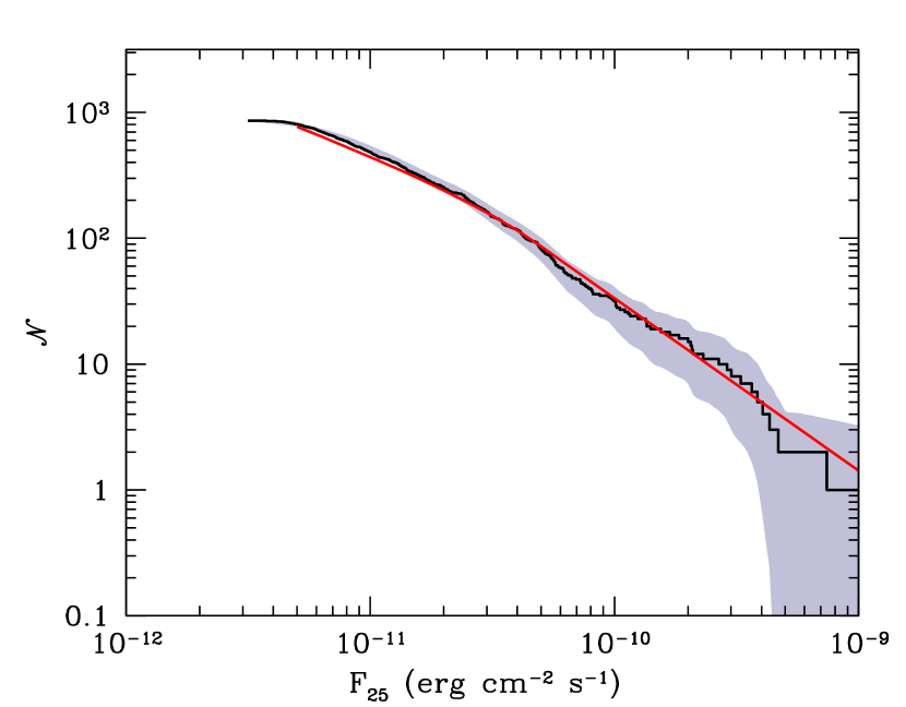
Figure 4: $\log\mathcal{N}$-$\log S$ relation defined in terms of $\mathcal{F}_{25}$ (top) and $F_{25}$ (bottom) for the Fermi blazars in the 2LAC. The shaded region provides an estimate of the 2$\sigma$ uncertainty in the Fermi $\log\mathcal{N}$-$\log S$ relation due to the measurement uncertainty on $F_{25}$ and the Poisson fluctuations in the sample itself. The empirically reconstructed $\log\mathcal{N}$-$\log S$ relation from Singal et al. (2012) is shown by the red line. For the latter, the Singal et al. (2012) $\log\mathcal{N}$-$\log S$ relation has been inferred using the average spectral index, $2.13$.

Figure 4 shows the $\log\mathcal{N}$-$\log S$ relation for all of the Fermi blazars in the 2LAC with a SNR $\geq 7$, defined in terms of $\mathcal{F}_{25}$ and $F_{25}$. The precision with which the $\log\mathcal{N}$-$\log S$ relation can be reconstructed empirically is limited by both the intrinsic measurement uncertainty (in $\mathcal{F}_{35}$ and $\Gamma_{F}$) and the limited number of AGN. We attempt to assess this uncertainty via a Monte Carlo simulation of the Fermi catalog, using the reported measurement uncertainties (assuming a normal and log-normal error distributions for $\Gamma$ and $\mathcal{F}_{35}$, respectively) and constructing bootstrap samples of the 2LAC. The 2$\sigma$ regions are shown by the gray shaded regions in Figures 4 and 5. However, we note that the errors at various fluxes are strongly correlated due to the cumulative definition of $\mathcal{N}(S)$, and thus must be interpreted cautiously.

The $F_{25}$ $\log\mathcal{N}$-$\log S$ relation is in good agreement with the empirically constructed $\log\mathcal{N}$-$\log S$ relation from Singal et al. (2012), providing some confidence in our reconstructed $F_{25}$ itself. Clearly evident in both forms of the $\log\mathcal{N}$-$\log S$ relation is a flattening at small fluxes. Singal et al. (2012) identify this with a systematic bias induced by a correlation between the $\mathcal{F}_{25}$ flux limit and the source spectral index, resulting in fewer soft sources being detected below a few$\times 10^{-8}\,{\rm photons~{}cm^{-2}~{}s^{-1}}$ (see Figure 14 of Ackermann et al., 2011). This results in a break in the $\log\mathcal{N}$-$\log S$ relation roughly at the value for $\mathcal{F}_{25}$ at which the sample becomes incomplete. Unlike $\mathcal{F}_{25}$, the flux limit in $F_{25}$ is only weakly dependent upon $\Gamma_{F}$ (cf. Figures 14 & 15 in Ackermann et al., 2011), and the break is correspondingly weaker.

Despite the known bias, Singal et al. (2012) have argued based upon the 1LAC that the intrinsic $\log\mathcal{N}$-$\log S$ relation does indeed have a break near $\mathcal{F}_{25}=6\times 10^{-8}~{}{\rm photons~{}cm^{-2}~{}s^{-1}}$. We believe this is suspect for three reasons. First, its location is very near the bias-induced break in the 1LAC. Second, the location of the break in the $\log\mathcal{N}$-$\log S$ relation constructed from the 2LAC blazars appears to have moved towards marginally lower fluxes. Third, the break is considerably less prominent when a less biased flux is employed, namely $F_{25}$. This points to an as yet unidentified source of bias for $F_{25}\lesssim 10^{-11}~{}{\rm erg~{}cm^{-2}~{}s^{-1}}$, and thus we will restrict ourselves to fluxes above this cutoff.

The $F_{25}$ $\log\mathcal{N}$-$\log S$ relation for the Fermi hard gamma-ray blazars specifically is shown in Figure 5. Aside from the restriction to blazars with $\Gamma_{F}<2$, this is constructed in an identical fashion to those described above. Apart from the reduced number of sources, it shares many of the qualitative features found for the $\log\mathcal{N}$-$\log S$ relation from the full blazar sample. In particular, the same suspect flattening for $F_{25}\lesssim 10^{-11}~{}{\rm erg~{}cm^{-2}~{}s^{-1}}$ is observed.

Associated with $\mathcal{N}(F_{25})$ is an estimate for the blazar contribution to the unresolved Fermi background, arising from the faint end of the blazar population:

$$F_{25,\rm tot}=\int_{0}^{\infty}dF_{25}\frac{d\mathcal{N}}{dF_{25}}F_{25}\,.$$ (13)

This provides an independent constraint upon the overall normalization, once resolved point sources have been removed. The associated Fermi limit upon $\mathcal{F}_{25,\rm tot}$ is $18\pm 2.4\times 10^{-5}~{}{\rm ph~{}cm^{-2}~{}s^{-1}}$, while that implied by the $\log\mathcal{N}$-$\log S$  relation in Singal et al. (2012) is $11\times 10^{-5}~{}{\rm ph~{}cm^{-2}~{}s^{-1}}$. Note the condition that $F_{25,\rm tot}$ be finite implies that $\mathcal{N}$ cannot be well approximated by a single power law. Above $F_{25}\simeq 10^{-11}~{}{\rm erg~{}cm^{-2}~{}s^{-1}}$, Singal et al. (2012) found $\mathcal{N}\propto F_{25}^{-1.37\pm 0.13}$, which were it to continue indefinitely to small fluxes would imply that $F_{25,\rm tot}$ diverges at the faint end.

3.1.2 Relationship to $\tilde{\phi}_{B}$

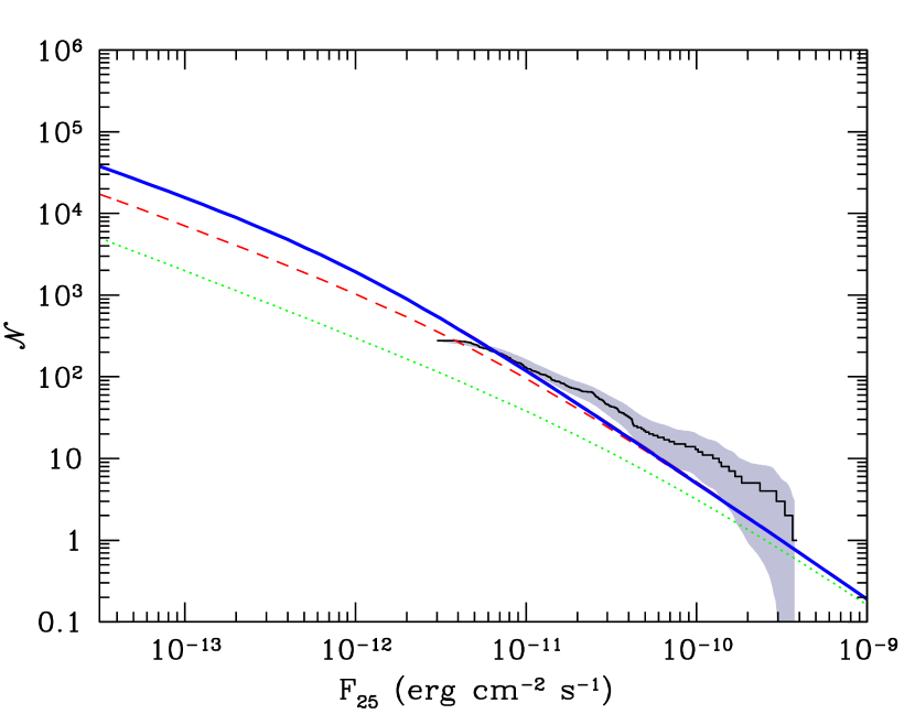
Figure 5: $\log\mathcal{N}$-$\log S$ relation in terms of the flux from 100 MeV – 100 GeV associated with the expanded hard gamma-ray blazar luminosity function presented in Equation (6) in comparison with that from the 2LAC Fermi hard gamma-ray blazar sample. The shaded region provides an estimate of the 2$\sigma$ uncertainty in the Fermi $\log\mathcal{N}$-$\log S$ relation due to the measurement uncertainty on $F_{25}$ and the Poisson fluctuations in the sample itself. The flattening in the Fermi $\log\mathcal{N}$-$\log S$ relation at low fluxes is probably an artifact of the Fermi flux limit. For reference, the contributions to the $\log\mathcal{N}$-$\log S$ relation from hard gamma-ray blazars with $z\leq 0.1$ (green dotted) and $z\leq 0.3$ (red dashed) are shown.

The primary difficulty in producing a $\log\mathcal{N}$-$\log S$ relation to compare with that constructed using the Fermi 2LAC blazars is the treatment of the particular selection effects relevant for the population of interest. Specifically, it is necessary to produce cuts on $\Gamma_{F}$ and $F_{25}$. Thus, we define

$$\mathcal{N}=\eta_{F}\int_{0}^{2}d\Gamma_{l}\int_{0}^{\infty}dz\int_{\log_{10}L_{\rm TeV}(F_{25},z,\Gamma_{l})}^{\infty}d\log_{10}L_{\rm TeV}\\ 4\pi D_{A}^{2}\frac{dD_{P}}{dz}\Theta\left[2-\Gamma_{F}(\Gamma_{l},z)\right]\tilde{\phi}_{B}(z,L_{\rm TeV},\Gamma_{l})\,,$$ (14)

where $L_{\rm TeV}(F_{25},z,\Gamma_{l})$ is given by Equation (10), $\Gamma_{F}(\Gamma_{l},z)$ is obtained as described in Section 2.2.2, $\Theta(x)$ is the Heaviside function (vanishing for $x<0$ and unity otherwise), and the cuts on $\Gamma_{l}$ and $\Gamma_{F}$ are motivated by Section 2.2.3 (note that the cut on $\Gamma_{l}$ is redundant). The coefficient $\eta_{F}=0.826$ is the correction due to the sky-coverage of the Fermi clean sample ($|b|>10^{\circ}$, where $b$ is the Galactic latitude). This is compared to the observed Fermi $\log\mathcal{N}$-$\log S$ relation for the hard gamma-ray blazars in Figure 5.

The cutoff in $\Gamma_{F}$ results in a $\Gamma_{l}$-dependent redshift cut, which is exhibited as a break in the $\log\mathcal{N}$-$\log S$ relation that moves to progressively larger fluxes as $\Gamma_{l}$ increases. This is evident in the $\log\mathcal{N}$-$\log S$ relations for sources restricted to smaller redshifts in Figure 5 (the green dotted and red dashed lines). As seen in Figure 3, the location of this redshift limit is sensitively dependent upon $\Gamma_{l}$, ranging between 0 and $\sim 1$ for $\Gamma_{l}$ from 2.0 to $\sim 1.4$. The $\Gamma_{l}$ sensitivity of the location of this break is part of the justification for the using the extended luminosity function in Equation (6). The location of the resulting break after integrating over the TeV blazar $\Gamma_{l}$ distribution is near $F_{25}=1.6\times 10^{-12}~{}{\rm erg~{}cm^{-2}~{}s^{-1}}$, roughly a factor of three below Fermi’s stated flux limit for the 2LAC, and a factor of six below the point at which unknown systematic effects appear to produce an artificial flattening of the Fermi $\log\mathcal{N}$-$\log S$ relation.

Above and below the break we obtain $\mathcal{N}\propto F_{25}^{-1.42}$ and $\mathcal{N}\propto F_{25}^{-0.75}$, respectively. Notably, despite the difference in the location of the cutoff, both of the power laws are consistent with those reported in Singal et al. (2012). In the case of the latter, however, we suspect the agreement is incidental.

Above a flux of $F_{25}=10^{-11}~{}{\rm erg~{}cm^{-2}~{}s^{-1}}$, the minimum flux at which we trust the Fermi $\log\mathcal{N}$-$\log S$ relation, Equation (14) reproduces the observed relation quite well. This is especially true for $F_{25}\lesssim 10^{-10}~{}{\rm erg~{}cm^{-2}~{}s^{-1}}$. At higher fluxes the paucity of sources induces large Poisson errors, and thus the excess bump at and above this flux is not significant.

Since we treat the hard gamma-ray blazar contributions to the EGRB in detail in Section 3.4, here we simply note that the anticipated contribution to the Fermi EGRB is $\mathcal{F}_{25,\rm tot}\simeq 1.19\times 10^{-5}~{}{\rm ph~{}cm^{-2}~{}s^{-1}}$. This corresponds to roughly 6.6% of the total Fermi EGRB from 100 MeV to 100 GeV, and 11% of that implied by the empirical reconstruction from the 1LAC by Singal et al. (2012). That the hard gamma-ray blazars are responsible for a such a small fraction of the EGRB is not surprising; below 10 GeV the EGRB is dominated by the FSRQs. Nevertheless, even at 100 MeV we expect the hard gamma-ray blazars to account for roughly 10% of the EGRB.

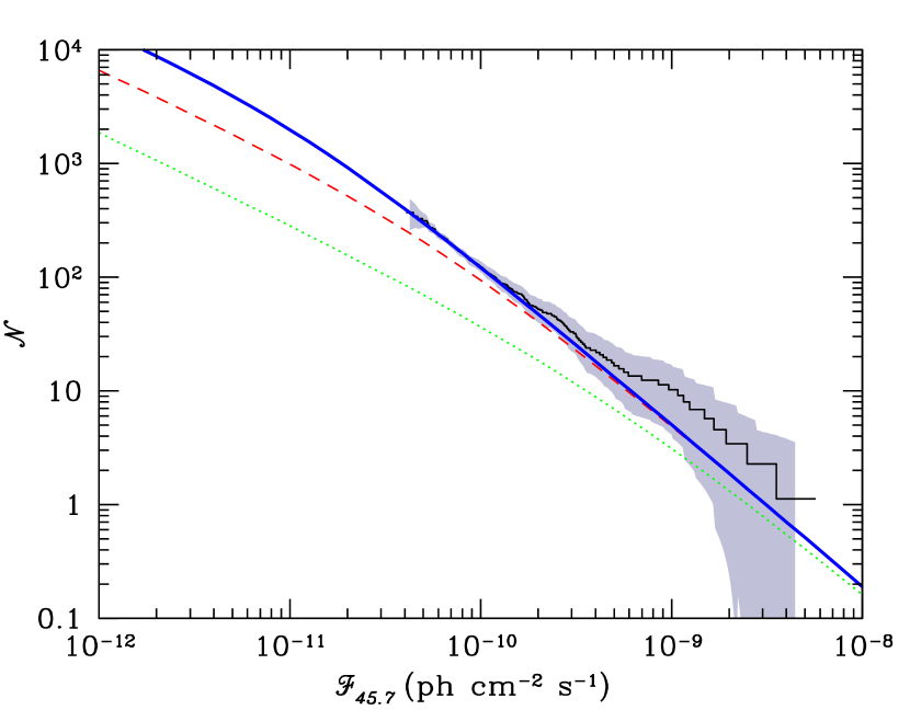
Figure 6: $\log\mathcal{N}$-$\log S$ relation in terms of the fluence from 10 GeV–500 GeV ($\mathcal{F}_{45.7}$) associated with the expanded hard gamma-ray blazar luminosity function presented in Equation (6) in comparison with that from the 1FHL Fermi hard gamma-ray BL Lac sample. The shaded region provides an estimate of the 2$\sigma$ uncertainty in the Fermi $\log\mathcal{N}$-$\log S$ relation due to the measurement uncertainty on $\mathcal{F}_{45.7}$ and the Poisson fluctuations in the sample itself. We have corrected for the detection efficiency following Ackermann et al. (2013), as described in Appendix C.1, and as a consequence the $\log\mathcal{N}$-$\log S$ relation does not show the artificial flattening at low fluxes exhibited in Figures 4 and 5. For reference, the contributions to the $\log\mathcal{N}$-$\log S$ relation from hard gamma-ray blazars with $z\leq 0.1$ (green dotted) and $z\leq 0.3$ (red dashed) are shown.

3.2 1FHL $\log\mathcal{N}$-$\log S$ Relation

Because the hard sources necessarily dominate at high energies, the recently published 1FHL, a catalog of Fermi sources detected above 10 GeV, provides a means to probe the hard-source population directly. Already it is clear that for hard sources the flattening at low fluxes is almost entirely, if not entirely, an artifact of the LAT detection efficiency near the flux threshold (see Appendix C.1 and Figures 31-33 of Ackermann et al., 2013). Thus, there is currently no evidence for a break in the $\log\mathcal{N}$-$\log S$ relation for the high-energy Fermi population.

As with the 2LAC sources, we may compare the $\log\mathcal{N}$-$\log S$ relation of 1FHL sources with that anticipated by the expanded luminosity function in Equation (6). Because the 1FHL reports the fluence between 10 GeV and 500 GeV explicitly ($\mathcal{F}_{45.7}$), eliminating the need to perform a spectral correction to this energy band, constructing the observed $\log\mathcal{N}$-$\log S$ relation within this energy band is somewhat simplified. It is, however, complicated by the fact that the 1FHL also includes a Galactic component that must be removed. We do this by considering only high latitude ($|b|>20^{\circ}$) sources that are identified as BL Lac objects. The resulting $\log\mathcal{N}$-$\log S$ relation is shown in Figure 6, and is comparable to Figure 33 of Ackermann et al. (2013).

The anticipated $\log\mathcal{N}$-$\log S$ relation is constructed in a manner similar to that in the previous section, replacing the relevant flux measure with $\mathcal{F}_{45.7}$, and adjusting the correction to account for the differing sky-coverage of the high-latitude 1FHL sample adopted. In addition, since the 1FHL detection efficiency is provided in Ackermann et al. (2013), we make an effort to correct the $\log\mathcal{N}$-$\log S$ relation near the detection threshold, as described in Section C.1. This is compared to the measured high-energy BL Lac $\log\mathcal{N}$-$\log S$ relation in Figure 6, providing an excellent fit over more than an order of magnitude in fluence. As with the 2LAC $\log\mathcal{N}$-$\log S$ relation shown in Figure 5, there is an excess of sources at high fluxes in the 1FHL, though again this is not significant. We do predict a weak break near $\mathcal{F}_{45.7}\simeq 2$–$3\times 10^{-11}~{}{\rm ph~{}cm^{-2}~{}s^{-1}}$, or roughly 50% of the fluence of the dimmest 1FHL source, and hence potentially accessible in the future.

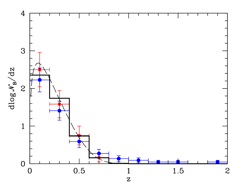
Figure 7: Nearby redshift distribution of the hard gamma-ray blazars above the Fermi flux limit anticipated by the luminosity function in Equation (6), both in continuous form (dashed) and binned with $\Delta z=0.2$ (continuous). For comparison the redshift distribution of the Fermi hard gamma-ray blazars in the 1LAC (red squares) and 2LAC (blue circles) are also shown. For these, the vertical error bars denote Poisson errors and the horizontal error bars denote bin sizes.

3.3 Hard Gamma-ray Blazar Redshift Distribution

In principle, the evolution in the number density of the nearby Fermi hard gamma-ray blazars is directly probed by their observed redshift evolution. As with the $\log\mathcal{N}$-$\log S$ relation, this is straightforward to define observationally. However, in practice, it is complicated by the flux-limited nature of the 2LAC, significantly impacting even moderate redshifts, and the limited number of sources with known redshifts (roughly 39%). Nevertheless, it represents a different projection of the hard gamma-ray blazar luminosity function, and provides a powerful additional test of the viability of a rapidly evolving blazar population.

Within the context of the 1LAC, we demonstrated in Paper I that the relatively large flux limit was capable of generating a precipitously declining observed number of blazars, $\mathcal{N}_{B}$, with redshift. However, there we made a number of assumptions and approximations regarding the intrinsic hard gamma-ray blazar spectra and their relationship to $L_{\rm TeV}$. Here we revisit this within the more complete 2LAC and in terms of the more fully self-consistent TeV blazar model described in Section 2. Particular improvements over the computation in Paper I are the self-consistent relationship between $L_{\rm TeV}$ and $F_{25}$, the distribution of $\Gamma_{l}$, and the ability to now dispense with the upper limit upon the TeV luminosity, to which our results are insensitive.

The definition of $\mathcal{N}_{B}(z)$ differs from $\mathcal{N}$ only by the limits of integration:

$$\mathcal{N}_{B}(z)=\int_{0}^{2}d\Gamma_{l}\int_{0}^{z}dz^{\prime}\int_{\log_{10}L_{\rm TeV}(F_{25,\rm min},z^{\prime},\Gamma_{l})}^{\infty}d\log_{10}L_{\rm TeV}\\ 4\pi D_{A}^{2}\frac{dD_{P}}{dz^{\prime}}\Theta\left[2-\Gamma_{F}(\Gamma_{l},z^{\prime})\right]\tilde{\phi}_{B}(z^{\prime},L_{\rm TeV},\Gamma_{l})\,,$$ (15)

where $F_{25,\rm min}\simeq 5\times 10^{-12}~{}{\rm erg~{}cm^{-2}~{}s^{-1}}$ is the flux limit of Fermi (see Figures 15 & 36 of Ackermann et al., 2011). As with the $\log\mathcal{N}$-$\log S$ relation, the spectral cut on $\Gamma_{F}$ induces a $\Gamma_{l}$-dependent redshift cutoff, limiting the potential contributions from very bright objects at high-$z$. This mimics the luminosity upper limit we applied in Paper I, removing its necessity. In practice, we compare $d\log\mathcal{N}_{B}/dz$, both to avoid correlations in the errors at subsequent redshifts and because the over-all normalization has already been compared in the context of the $\log\mathcal{N}$-$\log S$ relation.

Figure 7 shows the $d\log\mathcal{N}_{B}/dz$ for Fermi hard gamma-ray blazars with SNR $\geq 7$ in comparison to that inferred by Equation (15). As in Paper I, the agreement is quite good, though we miss what appears to be a small population of high-redshift objects. This may suggest an issue with our estimation of $\Gamma_{F}(z,\Gamma_{l})$, our distribution in $\Gamma_{l}$, and/or with the source identification in the 2LAC at high $z$. Alternatively, it may suggest a possibly faster evolution for blazars in comparison with quasars, as is the case for jet sources (i.e., radio-loud quasars, see, e.g., Singal et al., 2011, 2013). In any case, it is clear that a rapidly evolving TeV blazar population is explicitly consistent with the observed $d\log\mathcal{N}_{B}/dz$. As with the $\log\mathcal{N}$-$\log S$ relation, and unlike Paper I, there are no longer any free parameters.

3.4 Isotropic Extragalactic Gamma-ray Background

In contrast to the $\log\mathcal{N}$-$\log S$ relation and redshift distribution of Fermi blazars, the Fermi isotropic EGRB directly probes the population of unresolved gamma-ray blazars at high-$z$. Since a quasar-like evolution of the blazar population has the most dramatic effect at $z\sim 1$–2, limits upon such an evolution have historically come from modeling the EGRB.

The Fermi EGRB spectrum is constructed following Section 5.3 of Paper I, the only distinction being the subsequent average over $\Gamma_{l}$. We first define a TeV-luminosity normalized intrinsic spectrum:

$$\hat{I}_{E}=\frac{E\,(dN/dE)}{\int_{0.1~{}{\rm TeV}}^{10~{}{\rm TeV}}dE\,E\,(dN/dE)}\,,$$ (16)

in terms of which, the EGRB spectrum is

$$E^{2}\frac{d\bar{N}}{dEd\Omega}=\frac{E}{4\pi}\int_{0}^{2}d\Gamma_{l}\int_{z_{\rm 2LAC}}^{\infty}dz\int_{0}^{\infty}d\log_{10}L_{\rm TeV}\\ 4\pi D_{A}^{2}\frac{dD_{P}}{dz}\frac{L_{\rm TeV}}{4\pi D_{L}^{2}}\hat{I}_{E(1+z)}e^{-\tau(E,z)}\tilde{\phi}_{B}(z,L_{\rm TeV},\Gamma_{l})\,,$$ (17)

To exclude identifiable point sources we impose a lower redshift cutoff set by when the peak of the luminosity function, at isotropic equivalent luminosity of $\sim 2\times 10^{45}~{}{\rm erg~{}s^{-1}}$, passes the 2LAC, flux limit, approximately at $z_{\rm 2LAC}\simeq 0.291$. This is slightly larger than the $z_{\rm 1LAC}\simeq 0.25$ chosen in Paper I owing to the increased sensitivity limit of the 2LAC, which after two years should have a flux limit roughly $\sqrt{2}$ lower and thus related by $D_{L}^{2}(z_{\rm 2LAC})=\sqrt{2}D_{L}^{2}(z_{\rm 1LAC})$.

Important modifications to the intrinsic hard gamma-ray blazar spectra are the absorption above $\sim 1$ TeV due to the extragalactic background light (EBL) and the removal of identifiable point sources. As mentioned earlier, it is in the treatment of the former that our approach differs from other efforts to constrain the hard gamma-ray blazar population: here we assume that this energy is primarily dumped into the IGM as heat, instead of being reprocessed to lower energies by the inverse Compton cascades. Both the unabsorbed and point source uncorrected spectra are shown in Figure 8 for comparison.

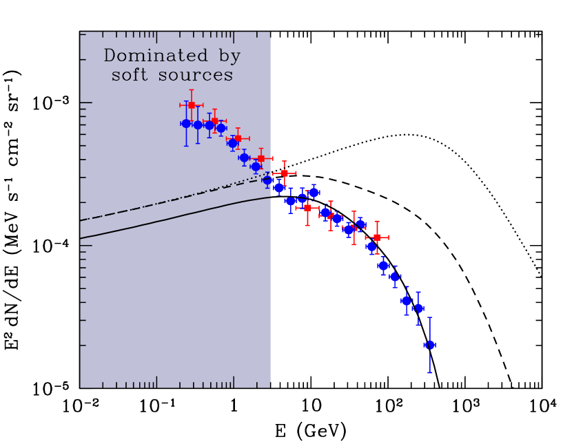
Figure 8: Fermi isotropic EGRB anticipated by the hard gamma-ray blazars. The dotted, dashed, and solid lines correspond to the unabsorbed spectrum, spectrum corrected for absorption on the EBL, and spectrum corrected for resolved point sources (assuming all hard gamma-ray blazars with $z\lesssim 0.291$ are resolved, see text). These are compared with the measured Fermi EGRB reported in Abdo et al. (2010a, red squares) and Ackermann et al. (2012b, blue circles). Note that below $\sim 10$ GeV the EGRB is dominated by soft sources, specifically, the Fermi FSRQs.

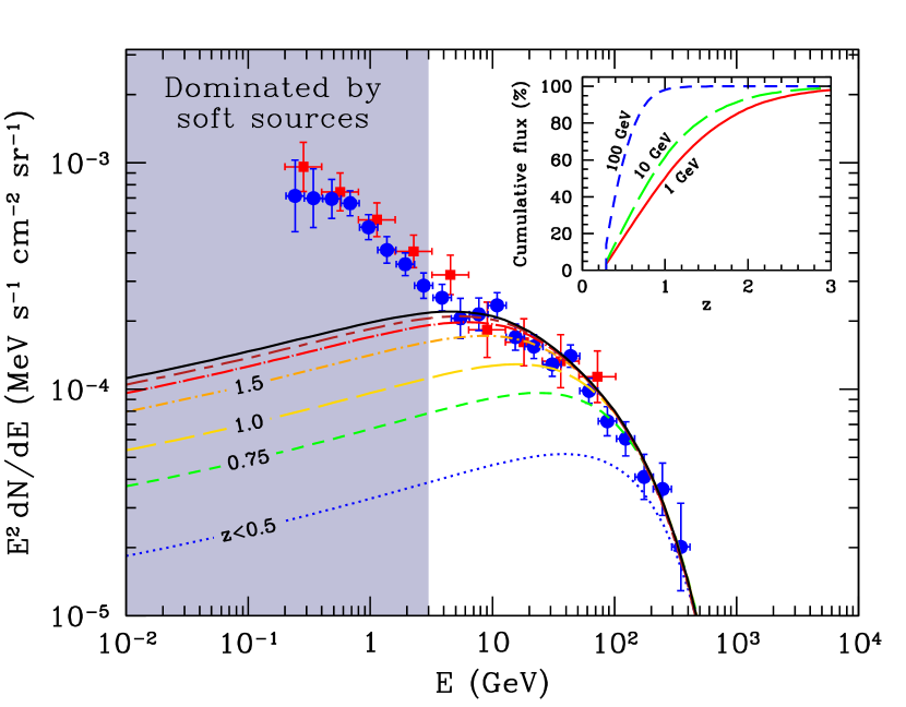
Figure 9: Contribution to the Fermi EGRB from hard gamma-ray blazars below various redshifts. Specifically, for objects with $z<0.5$ (blue dot), 0.75 (green short dash), 1.0 (yellow long dash), 1.5 (orange short dash dot), 2.0 (red long dash dot), 2.5 (dark red long dash-short dash), and all redshifts (black solid). In all cases it was assumed that all sources with $z\lesssim 0.291$ are resolved. These are compared with the measured Fermi EGRB reported in Abdo et al. (2010a, red squares) and Ackermann et al. (2012b, blue circles). Note that below $\sim 10$ GeV the EGRB is dominated by soft sources, specifically, the Fermi FSRQs. The inset shows the cumulative flux fraction as a function of redshift for 1 GeV (red solid), 10 GeV (green long dash), and 100 GeV (blue short dash).

Combined with absorption and point source identification, the high value of $\Gamma_{h}$ measured in bright TeV sources implies that the EGRB must be substantially suppressed above a TeV. That is, the power-law behavior implied by the Abdo et al. (2010a) measurement of the Fermi EGRB cannot extend significantly beyond the 100 GeV upper limit for which it was reported. This is seen explicitly in Figure 8, where for the distribution of $\Gamma_{l}$ adopted in Section 2.2.1 the anticipated contribution to the EGRB peaks near 10 GeV followed by a rapid decline at larger photon energies. This provides a remarkable agreement with the recent estimate of Fermi EGRB spectrum by Ackermann et al. (2012b), shown by the blue circles in in Figure 8. Moreover, the spectrum of the EGRB above 6 GeV appears to show a high energy bump upon a monotonically decreasing spectrum, which we identify with the specific population of hard gamma-ray blazars.

Even in the presence of substantial absorption, the bulk of the EGRB is produced at high redshifts, seen explicitly in Figure 9. At 10 GeV, roughly half of the observed EGRB is due to objects with $z>1$. The typical redshifts that contribute are necessarily energy-dependent, with the higher energy EGRB arising from more nearby sources. Nevertheless, it is clear that even above a few GeV the Fermi EGRB is probing the high-redshift blazar population.

The contribution to the EGRB spectrum from the hard gamma-ray blazars below 10 GeV is nearly flat, and consequently dominates their contribution to $\mathcal{F}_{25}$, consisting of roughly 10%, and responsible for the value obtained in Section 3.1. However, this number is quite uncertain, depending upon the behavior of the extension of the gamma-ray blazar luminosity function to $\Gamma_{l}>2$.

Below a few GeV the Fermi EGRB is dominated by soft gamma-ray sources, the most important of which are the FSRQs (see, e.g., Cavadini et al., 2011; Stecker & Venters, 2011). Their intrinsically soft spectra combined with their typically larger luminosities (and thus higher redshifts) confine their contribution to below $\sim 3$ GeV. Thus, our neglect of these sources is unlikely to significantly change the Fermi EGRB above 10 GeV, where the hard gamma-ray blazars successfully reproduce the observed background.

We note that the overall normalization of the TeV blazar luminosity density is subject to an uncertain correction factor that depends primarily on the incomplete census of the observed TeV blazar population and enters linearly into the overall normalization of the EGRB. We estimated this correction factor using the source counts of hard Fermi blazars and confirm its value by comparison to the redshift and cumulative flux distributions of these objects. Nevertheless, there are remaining uncertainties associated with the contribution of sources without measured redshifts and with the extrapolation of that population of the Fermi band to TeV energies. If another plausible source population such as starburst galaxies contributes a non-negligible, but subdominant, signal to the EGRB, it could be accommodated by a modest rescaling of the TeV luminosity density or slight modification to the hard gamma-ray blazar redshift evolution. Despite this uncertainty, the impressive match between the EGRB shape at energies above $\sim 3$ GeV strongly suggest that it is dominated by a rapidly evolving hard gamma-ray blazar population.

3.5 Anisotropy of the Extragalactic Gamma-ray Background

In principle, the anisotropy of the EGRB limits the potential contribution from discrete sources, providing a second direct constraint on the fraction of the EGRB associated with blazars. The angular power in the EGRB on small angular scales is observed to be roughly constant, consistent with the expected Poisson noise due to an unclustered population of point sources (Ackermann et al., 2012a). The magnitude of the angular power spectrum is energy dependent, yielding an EGRB anisotropy spectrum, $C_{P}(E)$, shown by the grey bars in Figure 10.

The origin of the constraint is straightforward to understand: large numbers of blazars result in large Poisson fluctuations, and therefore correspondingly large values of $C_{P}$. Similarly, the anisotropy spectrum’s energy dependence is directly associated with the underlying intrinsic spectra of the blazars: hard blazar spectra produce hard anisotropy spectra. The particular value of the EGRB anisotropy depends, however, upon which sources are included. Here we follow Cuoco et al. (2012) and compute the anisotropy associated with subsets of sources unresolved by the First Year Fermi-LAT Source Catalog (1FGL), corresponding roughly to a 1 GeV–100 GeV fluence limit of $\mathcal{F}_{35}^{\rm 1FGL}=5\times 10^{-10}\,{\rm ph~{}cm^{-2}~{}s^{-1}}$ (though see Appendix C.2 for detailed estimates of the fluence-dependent detection efficiency).

In terms of the TeV blazar luminosity function, the expected EGRB anisotropy due to the hard gamma-ray blazars within an energy band bounded by $E_{m}$ and $E_{M}$ is given by

$$C_{P,mM}=\int_{0}^{\Gamma}d\Gamma_{l}\int_{0}^{\infty}dz\int_{-\infty}^{\infty}d\log_{10}L_{\rm TeV}\\ 4\pi D_{A}^{2}\frac{dD_{P}}{dz}\mathcal{F}^{2}_{mM}\tilde{\phi}_{B}(z,L_{\rm TeV},\Gamma_{l})w(\mathcal{F}_{35})\,,$$ (18)

where $\mathcal{F}_{mM}$ is the fluence in the specified energy band, specified in Equation (8), with the energy range explicitly identified, and $w(\mathcal{F}_{35})$ is a weighting that describes the detection efficiency for the sample under consideration (see below).

In practice, the normalization of the EGRB anisotropy spectrum reported in Ackermann et al. (2012a) is inconsistent with the contributions arising from sources already resolved in the 2 Year Fermi LAT Source Catalog (2FGL). Detected sources in the 1FHL alone, without correcting for the 1FHL detection efficiency, are sufficient to account for the entirety of the reported EGRB anisotropy signal above 10 GeV (Broderick et al., 2013). Thus, consistency with the reported EGRB anisotropy would require a dramatic, and implausible, suppression in the $\log\mathcal{N}$-$\log S$ relation, shown in Figure 6, immediately below the 1FHL detection threshold.

It is possible, however, to unambiguously compare the anticipated hard gamma-ray blazar contribution to the EGRB anisotropy spectrum with either that from the 2FGL sources alone (for which an unambiguous estimate does exist) or simple extrapolations of the 2FGL source population (providing a reasonable upper limit). In the former, we consider the contribution to the EGRB arising from blazars that lie between the 2FGL and 1FGL detection thresholds. In the latter we consider all sources below the 1FGL flux limit, but compare the result to the EGRB anisotropy due to the power-law extrapolation of the 2FGL fluence distribution described in Broderick et al. (2013).

These comparisons are distinguished by the form of the weighting function, $w(\mathcal{F}_{35})$, appearing in Equation (18), which in both cases may be constructed from the detection efficiencies of the 1FGL and 2FGL, $\epsilon_{\rm 1FGL}(\mathcal{F}_{35})$ and $\epsilon_{\rm 2FGL}(\mathcal{F}_{35})$, respectively (explicit expressions for these are provided in Appendix C.2). In the case of the power-law extrapolation we need only to exclude sources that are detected in the 1FGL, i.e., $w(\mathcal{F}_{35})=1-\epsilon_{\rm 1FGL}(\mathcal{F}_{35})$. When comparing to the 2FGL contribution, we must also consider the probability that sources are detected in the 2FGL, thus $w(\mathcal{F}_{35})=[1-\epsilon_{\rm 1FGL}(\mathcal{F}_{35})]\epsilon_{\rm 2FGL}(\mathcal{F}_{35})$.

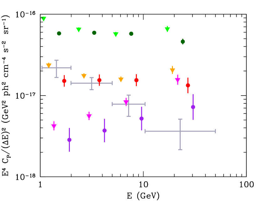
Figure 10: Various estimates of the EGRB anisotropy spectrum compared with that anticipated by the hard gamma-ray blazar luminosity function in Equation (6). The estimates associated with the power-law extension of the 2FGL, the 2FGL alone, and hard sources ($\Gamma_{F}<2$) within the 2FGL, are shown by the green, orange, and magenta triangles (left to right). The corresponding expectations from the hard gamma-ray blazars are shown by the dark green, red, and purple circles (left to right). In all cases bars denote the 1$\sigma$ cosmic variance uncertainty. For reference, the grey bars show the energy bins employed and values reported in Ackermann et al. (2012a), though see Broderick et al. (2013) regarding a discussion of their normalization. Points are horizontally offset within each bin for clarity.

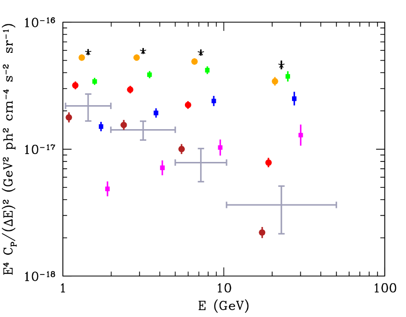
Figure 11: Cumulative contributions of various redshifts and intrinsic photon spectral index ($\Gamma_{l}$) to the EGRB anisotropy spectra. Contributions from sources with $z>0.291$, 1, and 1.5 are shown by the orange, red, and dark red circles, respectively (right to left within each energy bin). Contributions from objects with $\Gamma_{l}<1.9$, 1.8, and 1.7, are shown by the green, blue, and magenta squares, respectively (left to right within each energy bin). For comparison, the black star shows the EGRB anisotropy spectrum associated with all sources. In all cases bars denote the 1$\sigma$ cosmic variance uncertainty. For reference, the grey bars show the energy bins employed and values reported in Ackermann et al. (2012a), though see Broderick et al. (2013) regarding a discussion of their normalization. Points are horizontally offset within each bin for clarity.

The EGRB anisotropy implied by the hard gamma-ray blazar luminosity function in Equation (6) is significantly larger than the values reported in Ackermann et al. (2012a) in all energy bands. This is unsurprising given that the reported values appear to be a substantial underestimate of the EGRB anisotropy spectrum itself (Broderick et al., 2013). Nevertheless, it is consistent with (i.e., lies below) the values anticipated from a smooth power-law extrapolation of the 2FGL, shown in Figure 10. More importantly, a similar conclusion follows from the comparison to the contribution to the EGRB anisotropy from the 2FGL sample alone. This holds for both the full 2FGL sample and the sub-sample of hard sources (i.e., $\Gamma_{F}<2$). Thus, despite being inconsistent with the reported values in Ackermann et al. (2012a), the hard gamma-ray blazar luminosity function in Equation (6) is able to reproduce the inferred anisotropy signal associated with the currently known and smoothly extrapolated point source samples, respectively.

The $C_{P,mM}$ are dominated by nearby sources, i.e., $z\lesssim 1$. This is clearly seen in Figure 11, in which the contribution from sources with $z>1$ is below 33% above 1.99 GeV, and rapidly decreasing with redshift cut. As a result, unlike the isotropic EGRB component, the EGRB anisotropy is a probe of the nearby blazar distribution (immediately below the 1FGL, and above the 2FGL, detection thresholds). This is a direct result of the dominance of sources near the detection threshold in the definition of the $C_{P,mM}$. Hence, the agreement with the 2FGL contribution to the anisotropy is largely anticipated by the success at reproducing the statistics of the low-redshift hard gamma-ray blazar sample described in Sections 3.1 and 3.3.

The fractional contribution of intrinsically hard sources increases with energy, though even in the highest energy bin (10.4 GeV–50 GeV) sources with $\Gamma_{l}<\bar{\Gamma}_{l}$ contribute less than half of the anisotropy signal (see the blue squares in Figure 11). Therefore, even a moderate restriction on $\Gamma_{l}$ produces a substantial reduction in the anisotropy at all energies, implying that our anisotropy estimates are sensitive to the high-$\Gamma_{l}$ extension of the gamma-ray blazar luminosity function. Despite this uncertainty, the hard gamma-ray blazars contribute substantially, if not dominantly, to the anisotropy above roughly 3 GeV, consistent with their contribution to the isotropic EGRB. That is, it is possible to simultaneously match both the isotropic and anisotropic components of the EGRB with the single hard gamma-ray blazar population postulated here.

It is tempting to conclude that the absence of inverse Compton cascades, which could be preempted by the presence of virulent plasma beam instabilities, enables a notable consistency within the context of the simplest model conceivable. That is, the resolved source class of hard gamma-ray blazars, which dominates the extragalactic high-energy regime, also dominates the angular power as well as matches the detailed shape and normalization of the isotropic EGRB intensity above 3 GeV. However, as noted above, the current ambiguity in the normalization of the reported EGRB anisotropy presently precludes such a statement in general. The consistency obtained in Figure 10 is largely degenerate with the success in reproducing the low-redshift gamma-ray blazar population. Given the dominance of low-redshift source contribution to the anisotropy, this is likely to continue to be the case in the future. As a result, even with the dramatic evolution in the blazar population posited here, the EGRB anisotropy will predominantly probe the low-redshift blazar distribution generally.

4 Conclusions

In contrast to previous claims, a quasar-like evolution in the number density of TeV blazars is fully consistent with the properties of the observed Fermi population. The chief uncertainties remain fundamentally astrophysical: 1. How to relate the fluxes within the Fermi-relevant energy range and the intrinsic TeV luminosity, used to define the TeV blazar luminosity function, and 2. The efficiency of the inverse Compton cascades, if present at all.

A broken power-law model for the intrinsic TeV blazar spectrum, with a generic break energy and high-energy photon spectral index of 1 TeV and 3, respectively, is sufficient to reproduce many of the features of the Fermi hard gamma-ray blazar population. The TeV blazar luminosity function was constructed for blazars that were observed at TeV energies and hence is fundamentally limited to spectra which peak near $\sim 1$ TeV, and thus we necessarily impose an upper cutoff in the low-energy photon spectral index of 2. This cutoff is empirically supported by the observed distribution of Fermi photon spectral indexes for the known TeV blazars.

Modeling systematic biases is crucial to relating the intrinsic blazar population and the Fermi blazar sample. Of these, the most important is the softening of the Fermi-band spectra due to absorption on the EBL, which causes a strong redshift-dependent evolution in the observed photon spectral index from 1 GeV–100 GeV. This, in turn, induces a significant sensitivity to the form of the intrinsic spectrum below 1 TeV, generally, and in our case the low-energy photon spectral index, specifically. For this reason, to obtain robust estimates of the anticipated $\log\mathcal{N}$-$\log S$ relation and redshift distribution of nearby Fermi hard gamma-ray blazars, we found it necessary to expand the definition of the TeV blazar luminosity function to include the low-energy spectral index distribution. This is well approximated by a Gaussian peaked at a photon spectral index of 1.78 and standard deviation 0.18. Due to the redshift-dependent spectral softening, the $\log\mathcal{N}$-$\log S$ relation and hard gamma-ray blazar redshift distribution both probe primarily $z\lesssim 1$.

The 2LAC $\log\mathcal{N}$-$\log S$ relation is well reproduced for 100 MeV–100 GeV fluxes above $10^{-11}~{}{\rm erg~{}cm^{-2}~{}s^{-1}}$. At smaller fluxes a catalog-dependent flattening of the $\log\mathcal{N}$-$\log S$ relation suggests the presence of an unidentified systematic effect similar to that described by Singal et al. (2012). We predict the presence of a break in the hard gamma-ray blazar $\log\mathcal{N}$-$\log S$ relation roughly at the current Fermi flux limit, $5\times 10^{-12}~{}{\rm erg~{}cm^{-2}~{}s^{-1}}$. However, the location of this break is determined primarily by objects near our low-energy photon spectral index cutoff ($\Gamma_{l}=2$), and thus is potentially sensitive to the unmodeled soft end of the TeV blazar luminosity function.

Both the shape and magnitude of the 1FHL $\log\mathcal{N}$-$\log S$ relation for 10 GeV–500 GeV fluences above $4\times 10^{-10}~{}{\rm ph~{}cm^{-2}~{}s^{-1}}$, presumably dominated by the hard, gamma-ray bright objects of interest here, is excellently reproduced, after correcting for the 1FHL detection efficiency. Again, we predict a break in the $\log\mathcal{N}$-$\log S$ relation at fluxes near the threshold, though the specific value is dependent upon the blazar luminosity function near photon spectral index cutoff, and is therefore somewhat uncertain.

Similarly, we are able to obtain a good fit to the Fermi 2LAC hard gamma-ray blazar redshift distribution. In contrast to similar calculations in Paper I, it is no longer necessary to specify an arbitrary $\Gamma_{l}$ relationship between the inferred Fermi-band and TeV luminosities, or maximum intrinsic TeV luminosity, substantially improving the robustness of the expected distribution. In comparison to that from the 2LAC, our $d\log\mathcal{N}_{B}/dz$ falls marginally faster, either due to our assumption of a fixed-flux cutoff or suggesting an even more radical evolution of the TeV blazar luminosity function at low redshift.

In contrast to the $\log\mathcal{N}$-$\log S$ relation and the hard gamma-ray blazar redshift distribution, the Fermi EGRB directly probes the high-$z$ evolution of the TeV blazar luminosity function. Below $\sim 3$ GeV the FSRQs, and other soft sources, dominate the EGRB. However, above $\sim 3$ GeV, where soft sources contribute negligibly, the expected contribution from the hard gamma-ray blazars provide a remarkable fit to the most recently reported Fermi EGRB. Of particular importance is the now observed strong suppression above 100 GeV; due to absorption on the EBL this is a robust prediction of the TeV blazar luminosity function.

Simultaneously, the hard gamma-ray blazars reproduce the observed degree of anisotropy in the Fermi EGRB at energies where they dominate the isotropic component. This is possible since the anisotropic and isotropic components of the EGRB are probing the hard gamma-ray blazar population at different redshifts (being dominated by nearby bright and distant dim objects, respectively), with the disparity being precisely that anticipated by the rapidly evolving TeV blazar luminosity function we have posited (note that this implies this success may be largely degenerate with the ability to reproduce the statistics of the hard gamma-ray blazars at low redshifts). Thus, above $\sim 3$ GeV the Fermi EGRB may be fully explained within the context of the single resolved source class of hard gamma-ray blazars.

cccccccc Parameters of the Quasar Luminosity Function from Hopkins et al. (2007) Normalization $\log_{10}L_{*}$ $\gamma_{1}$ $\gamma_{2}$ $\log_{10}\phi_{*}$ a & $-4.825\pm 0.060$ $\left(\log_{10}L_{*}\right)_{0}$ b $13.036\pm 0.043$ $\gamma_{1,0}$ $0.417\pm 0.055$ $\gamma_{2,0}$ $2.174\pm 0.055$
$k_{L,1}$ $0.632\pm 0.077$ $k_{\gamma_{1}}$ $-0.623\pm 0.132$ $k_{\gamma_{2},1}$ $1.460\pm 0.096$
$k_{L,2}$ $-11.76\pm 0.38$ $k_{\gamma_{2},2}$ $-0.793\pm 0.057$
$k_{L,3}$ $-14.25\pm 0.80$
aIn units of co-moving ${\rm M}{\rm pc}^{-3}$ bIn units of $L_{\odot}\equiv 3.9\times 10^{33}\,{\rm erg}\,{\rm s}^{-1}$

The comparisons described above are based on an a priori model for the TeV blazar population, with no adjustable parameters. Thus, the success of the TeV blazar luminosity function is non-trivial; these are not “fits” in the normal sense. However, critical to these is the absence of the inverse Compton cascade emission that reprocesses the flux above $\sim$TeV into the Fermi-energy bands. If this occurs, the Fermi flux for a given TeV luminosity would increase substantially, moving the $\log\mathcal{N}$-$\log S$ relations towards higher fluxes, $d\log\mathcal{N}_{B}/dz$ towards higher $z$, the EGRB towards higher energy fluxes, the EGRB anisotropy towards higher variances, and thus in all cases badly violating the existing Fermi limits. Insofar as the evolution of TeV blazars may be expected to qualitatively reflect the cosmological history of accretion on to halos, this success may be seen as tentative support for the absence of the inverse Compton cascades, and thus presumably circumstantial evidence in favor of the existence of the only known alternative, beam plasma instabilities.

Appendix A An Explicit Expression for the Quasar Luminosity Function

In the interests of completeness, here we reproduce the co-moving quasar luminosity function, $\phi_{Q}(z,L)$ from Hopkins et al. (2007), corresponding to the “Full” case in that paper, that we employ. See Hopkins et al. (2007) for how this $\phi_{Q}(z,L)$ was obtained, and caveats regarding its application.

The form of $\phi_{Q}(z,L)$ is assumed to be a broken power law:

$$\phi_{Q}(z,L)=\frac{\phi_{*}}{[L/L_{*}(z)]^{\gamma_{1}(z)}+[L/L_{*}(z)]^{\gamma_{2}(z)}}\,,$$ (19)

where the location of the break ($L_{*}(z)$) and the power laws ($\gamma_{1}(z)$ and $\gamma_{2}(z)$) are functions of redshift. These are given by,

$$\log_{10}L_{*}(z) =\left(\log_{10}L_{*}\right)_{0}+k_{L,1}\xi+k_{L,2}\xi^{2}+k_{L,3}\xi^{3}$$ (20)

$$\gamma_{1}(z) =\gamma_{1,0}10^{k_{\gamma_{1}}\xi}$$

$$\gamma_{2}(z) =2\gamma_{2,0}\left(10^{k_{\gamma_{2},1}\xi}+10^{k_{\gamma_{2},2}\xi}\right)^{-1}$$

where

$$\xi\equiv\log_{10}\left(\frac{1+z}{3}\right)\,.$$ (21)

The values of the relevant parameters are given in Table 4. Finally, $\tilde{\phi}_{Q}$, defined in terms of physical volume, is related in the usual way:

$$\tilde{\phi}_{Q}(z,L)=(1+z)^{3}\phi_{Q}(z,L)\,.$$ (22)

Appendix B Explicit Flux Definitions

We employ three definitions of “flux” here: the fluences from 100 MeV–100 GeV ($\mathcal{F}_{25}$) and 1 GeV–100 GeV ($\mathcal{F}_{35}$) and the flux from 100 MeV–100 GeV ($F_{25}$). These are related to the reported $\mathcal{F}_{35}$ via Equations (11) and (12). Explicitly, setting $f_{F}$ with by $\mathcal{F}_{35}$,

$$f_{F}=\frac{\Gamma_{F}-1}{1-100^{1-\Gamma_{F}}}\mathcal{F}_{35}~{}{\rm GeV^{\Gamma_{F}-1}s^{-1}}\,,$$ (23)

the corresponding value for $\mathcal{F}_{25}$ is

$$\mathcal{F}_{25}=\frac{0.1^{1-\Gamma_{F}}-100^{1-\Gamma_{F}}}{1-100^{1-\Gamma_{F}}}\mathcal{F}_{35}\,,$$ (24)

where we have assumed $\Gamma_{F}\neq 1$. Similarly, $F_{25}$ is given by

$$F_{25}=\left\{\begin{aligned} &\frac{\Gamma_{F}-1}{\Gamma_{F}-2}\frac{0.1^{2-\Gamma_{F}}-100^{2-\Gamma_{F}}}{1-100^{1-\Gamma_{F}}}\mathcal{F}_{35}~{}{\rm GeV}&&\Gamma_{F}\neq 2\\ &\frac{\Gamma_{F}-1}{1-100^{1-\Gamma_{F}}}\log(10^{3})\mathcal{F}_{35}~{}{\rm GeV}&&\Gamma_{F}=2\,,\end{aligned}\right.$$ (25)

where the additional factor of a GeV sets the scale of the energy flux.

Appendix C Detection Efficiencies of High Latitude Gamma-ray Point Source Samples

Here we summarize the detection efficiencies associated with various high-latitude point source samples employed in the text.

C.1 1FHL

Figure 12: 1FHL Detection Efficiency for high-latitude sources ($|b|>15^{\circ}$), taken from Figure 30 of Ackermann et al. (2013).

In the construction of the 1FHL $\log\mathcal{N}$-$\log S$ relation we make an attempt to account for the detection efficiency using the values shown in Figure 30 of Ackermann et al. (2013). Specifically, we set

$$\mathcal{N}(S)=\sum_{j}\frac{1}{\epsilon(\mathcal{F}_{45.7})}\Theta(\mathcal{F}_{45.7}-S)$$ (26)

where $\epsilon(\mathcal{F}_{45.7})$ is the spline-interpolated detection efficiency shown in Figure 12.

C.2 1FGL and 2FGL

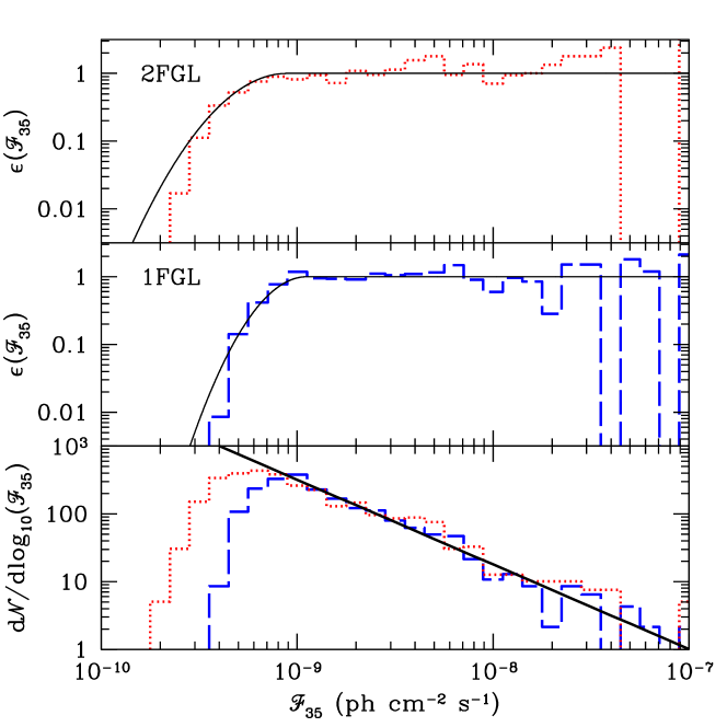
Figure 13: 1FGL and 2FGL Detection Efficiency for high-latitude sources ($|b|>15^{\circ}$). Bottom: $\mathcal{F}_{35}$ distributions of the 1FGL (blue dashed) and 2FGL (red dotted) in comparison to a power-law extrapolation of the latter (black solid). Middle and top: Estimates of the detection efficiencies of the 1FGL and 2FGL assuming the power-law extrapolation of the 2FGL approximates the true source flux distribution.

Unlike the 1FHL, the 1FGL and 2FGL point source detection efficiency are not present in the literature. However, these are necessary to reconstruct the anticipated EGRB anisotropy spectra associated with populations either masked by, or due to, these populations. Here we approximately reconstruct these detection efficiencies, following the procedure employed in Broderick et al. (2013) (to which we direct the reader for a more complete discussion).

Figure 13 shows the distribution of all sources with $|b|>15^{\circ}$ in the 1FGL and 2FGL catalogs in $\mathcal{F}_{35}$. This flux measure was chosen since it is both reported in the 1FGL and 2FGL catalogs and is apparently uncorrelated with the photon spectral index. Above $\mathcal{F}_{35}\simeq 10^{-9}~{}{\rm ph~{}cm^{-2}~{}s^{-1}}$ the two populations are both consistent with a single power law, $\propto\mathcal{F}_{35}^{-1.25}$. At lower fluences the number of 1FGL rapidly decreases. The extension of the 2FGL to even lower fluences, where it to exhibits a rapid decline, implies that these are associated with the detection efficiency of the respective catalogs and not with some intrinsic feature of the underlying source population.

Assuming that the high-fluence power law provides an approximation of the true source population, the ratio of the observed fluence distribution to the power law provides an estimate of the desired detection efficiency, $\epsilon(\mathcal{F}_{35})$. These are shown in the top two panels of Figure 13. We approximate the detection efficiencies by a

$$\epsilon(\mathcal{F}_{35})=\begin{cases}10^{-m[\log_{10}(\mathcal{F}_{35}/\mathcal{F}_{\rm max})]^{2}}&\mathcal{F}_{35}<\mathcal{F}_{\rm max}\\ 1&\text{otherwise}\,,\end{cases}$$ (27)

where for the 1FGL we have $m^{\rm 1FGL}=7$ and $\mathcal{F}_{\rm max}^{\rm 1FGL}=1.12\times 10^{-9}~{}{\rm ph~{}cm^{-2}~{}s^{-1}}$, and for the 2FGL we have $m^{\rm 2FGL}=4$ and $\mathcal{F}_{\rm max}^{\rm 2FGL}=0.89\times 10^{-9}~{}{\rm ph~{}cm^{-2}~{}s^{-1}}$. These fits, shown in Figure 13, are most accurate in the immediate vicinity of the detection threshold, the region that dominates the contribution to the EGRB anisotropy measurements.

In these no attempt to correct for Eddington bias (Eddington, 1913, 1940) has been made, despite being evident in the 1FHL and 1FGL (resulting in $\epsilon>1$ near the fluence threshold, corresponding to lower-fluence sources being detected at higher fluences). Doing so would reduce the inferred EGRB anisotropies.