A multiscale modeling study for the convective mass transfer in a subsurface aquifer

Abstract

Quantitative and realistic computer simulations of mass transfer associated with CO₂ disposal in subsurface aquifers is a challenging endeavor. This article has proposed a novel and efficient multiscale modeling framework, and has examined its potential to study the penetrative mass transfer in a CO₂ plume that migrates in an aquifer. Numerical simulations indicate that the migration of the injected CO₂ enhances the vorticity generation, and the dissolution of CO₂ has a strong effect on the natural convection mass transfer. The vorticity decays with the increase of the porosity. The time scale of the vertical migration of a CO₂ plume is strongly dependent on the rate of CO₂ dissolution. Comparisons confirm the near optimal performance of the proposed multiscale model. These primary results with an idealized computational model of the CO₂ migration in an aquifer brings the potential of the proposed multiscale model to the field of heat and mass transfer in the geoscience.

keywords:mass transfer multiscale modeling porous media CO₂ plume subsurface flow aquifer wavelet method numerical modeling.

List of symbols
$C$	Concentration of CO2
$C_{0}$	Reference concentration of CO2
$D$	Diffusion coefficient ($\mathrm{m^{2}s^{-1}}$)
$d$	Microscopic length scale ($\mathrm{m}$)
$g$	Acceleration due to gravity ($\mathrm{ms^{-2}}$)
$H$	Vertical length scale of the aquifer ($\mathrm{m}$)
$K$	Permeability ($\mathrm{m^{2}}$)
$L$	Horizontal length scale of the aquifer ($\mathrm{m}$)
$M$	Molar mass of CO2 ($\mathrm{kg/mol}$)
$N$	Number of nodes on a regular mesh
$\mathcal{N}$	Number of nodes on an adaptive mesh
$N_{b}$	Buoyancy frequency ($\mathrm{s^{-1}}$)
$\mathcal{D}a$	Darcy number, $\frac{K}{H^{2}}$
$\mathcal{R}e$	Reynolds number at macroscale, $\frac{UH}{\nu}$
$\mathcal{R}e_{d}$	Reynolds number at pore scale, $\frac{Ud}{\nu}$
$\mathcal{S}c$	Schmidt number, $\frac{\nu}{D}$
$u_{D_{i}}$	Space-time mean Darcian velocity ($\mathrm{ms^{-1}}$)
$\langle\overline{u}_{i}\rangle$	Space-time mean intrinsic velocity ($\mathrm{ms^{-1}}$)
$u^{\prime}_{i}$	Deviation from $u_{D_{i}}$ in a REV ($\mathrm{ms^{-1}}$)
$u^{\prime\prime}_{i}$	Deviation from $\langle\overline{u}_{i}\rangle$ in a REV ($\mathrm{ms^{-1}}$)
$u_{1},u_{3}$	Dimensionless space-time mean intrinsic velocity
$c$	Dimensionless space-time mean intrinsic concentration
$x_{i}$	Cartesian coordinate in the $i$-th direction
Greek symbols
$\alpha$	Ratio of molecular viscosity to effective viscosity
$\beta$	Solutal expansion coefficient
$\Gamma$	Rate of CO2 dissolution ($\mathrm{Mm^{-1}}$)
$\Delta V$	Representative elementary volume (REV)
$\Delta V_{f}$	The fraction of REV occupied with fluid
$\Delta t$	time step
$\Delta x_{i}$	Local step size in the $x_{i}$ direction
$\Delta x$	Minimum of $\Delta x_{i}$ for $i=1,\,3$
$\phi$	Porosity $\left(\frac{\Delta V_{f}}{\Delta V}\right)$
$\rho_{0}$	Reference density
$\lambda$	Characteristic length scale of a REV
$\epsilon$	Error tolerance
$\mu$	Molecular viscosity ($\mathrm{kgs^{-1}m^{-1}}$)
$\nu$	Kinematic viscosity ($\mathrm{m^{2}s^{-1}}$)

1 Introduction

The natural and mixed convection heat and mass transfer is an important topic of scientific scrutiny in a subsurface flow problem that investigates the disposal of anthropogenic CO₂ from the atmosphere into saline aquifers [33]. Example of such projects include the Utsira sand at Sleipner, Norway [12], the Mt. Simon aquifer in the Illinois basin [26, 4], saline aquifers in the Alberta basin, Canada [38], and the Carrizo-Willcox aquifer in Texas (CWT) [29]. Seismic data from the Sleipner shows a marked increase in the CO₂ flux near the reservoir top (see Fig 1$a$ of [12]), which suggests further investigation of the rate of vertical migration and progressive development of CO₂ plumes (e.g. [12]). Chadwick et al [12] hypothesized that this marked variability may be due to the multiscale natural convection mass transfer associated with the non-Darcian plume migration through numerous pathways in the aquifer. In the same vein, multiscale processes associated to a plume migration in the Carrizo-Willcox aquifer was investigated numerically by Pruess and Nordbotten [37] using a classical macroscopic Darcian model along with a sub-grid scale parameterization scheme (albeit the exact form of the scheme was not outlined with full details in [37]). Clearly, a complete understanding of the multiscale mass transfer mechanism in aquifers remains an active research area in the field of geoscience and reservoir engineering [29, 37, 27, 40, 16, 34, 15]. Hence, there are increasing interests on extending the adaptive mesh and multiscale finite volume/element methods (AMR based methods) for high performance numerical simulations of flow and transport in saline aquifers (e.g., see, [16, 20, 24, 30, 31, 23, 34, 15]).

The present article has investigated the development of a novel adaptive wavelet multiscale modeling and simulation methodology for studying the non-Darcian flow and transport through aquifers. One objective of this article is to investigate an effective methodology to minimize computation work and to improve the accuracy for transport problems in aquifers that deal with multiscale phenomena, in comparison to the commonly used classical numerical methods. For example, some authors verified with a classical method that a $\Delta x$ between $5\times 10^{-4}~{}\mathrm{m}$ and $10^{-3}~{}\mathrm{m}$ is necessary to capture multiscale features (e.g., see [38, 37, 34]), for which, the number of the grid points is about $N=10^{13}$ in the domain $1~{}\mathrm{m}\times 5~{}\mathrm{m}$ (e.g. [38]), and hence, $N$ would be far beyond the limit of modern computers for such a faithful simulation in a vertical cross section ($100~{}\mathrm{km}\times 200~{}\mathrm{m}$) of the CWT [37]. In contrast, this article investigates a multiscale methodology to put the computational effort locally in the physical domain (see [44, 2, 3, 1, 47, 46] for a technical details), where it is necessary to adapt the computational work to field-scale geological structures and complex physical processes in aquifers.

In the same vein, AMR based classical adaptive and mutiscale methods require to find an individual error monitoring scheme for each new applications (e.g. [23, 24, 34]). These methods were developed for steady elliptic problems, and their extension to multiscale flow and transport in aquifers is being investigated by a number of other authors (see the recent work of Künze et al [24]). Note also that an extremely small time step ($\Delta t$) is needed when these AMR based methods explicitly simulate natural and mixed convection heat and mass transfer in aquifers. In contrast, the present article investigates a multiscale methodology that captures multiscale physics with a more robust wavelet based computation, where the error is controlled a priori according to a prescribed tolerance ($\epsilon$) [47, 46], and the time step ($\Delta t$) can be chosen independent of the spatial grid ($\Delta x$) [2, 3]. In addition, the present research employs the volumetric mean of the time-averaged conservation laws with respect to a representative elementary volume (REV) so that the non-Darcian multiscale features (e.g. [12]) in a flow may be resolved with a non-Darcian multiscale model (see [45, 14] and the refs therein). This approach provides a natural framework for adopting appropriate parameterization for phenomena which are not directly resolved with the mean conservation laws (e.g. [37]). Here, the effect of CO₂ dissolution on the gravitational segregation of a CO₂ plume has been parameterized. Most importantly, the size of the REV has been adapted dynamically to the local variation of the CO₂ mass fraction. To the best of knowledge, the present development is a first time investigation for the multiscale natural convection mass transfer in a saline aquifer, and it complements the growing trend in computational modeling of the natural/mixed convection phenomena in subsurface flows as well as in other fields [23, 31, 34, 36, 47, 46]. Following are few remarks on the proposed multiscale methodology.

Remarks:

• The flow and transport at the reservoir scale is approximated with the classical Darcian approach. The multiscale mass transfer has been resolved with a non-Darcian approach. Subgrid scale parameterization schemes for both the momentum diffusion and the CO₂ dissolution have been adopted.

• A multilevel algorithm has been developed for the nonlinear coupling between the mass and momentum transfer processes in aquifers, which occurs at different temporal and spatial scales.

• Spatial differential operators are discretized using $\mathcal{N}$ significant wavelets, where each wavelet represents the change in scale near a grid point, and multiscale features are captured with a multiscale wavelet theory.

• There are two important computational benefits. First, the number of grid points $\mathcal{N}$ is significantly small compared to the number of grid points needed for a classical numerical method if the same level of accuracy is desired. Second, if $\mathcal{N}$ increases, then the CPU time increases approximately linearly. Note that for a given tolerance $\epsilon$, $\mathcal{N}$ may increase due to change in gradients of solution.

• The error for such a simulation is controlled in both space and time according to the prescribed tolerance ($\epsilon$) and the maximum allowable CFL number, which is verified with a large number($>50$) of numerical experiments.

Section 2 summarizes the new developments towards capturing the multiscale features in a subsurface plume migration. The adaptive multiscale methodology has been presented in section 3. Representative results from a series of numerical experiments have been presented in section 4. Finally, section 5 discusses the potential extension of the present development in the field of computational heat and mass transfer analysis.

$(a)$	$(b)$

Figure 1: $(a)$ Observed volumes of CO₂ near the top of the Sleipner aquifer between $1999$ and $2006$; data 1: volume ($\mathrm{m}^{3}$) of CO₂ by method $1$, broken line: fitted curve, $t+t^{2}$, data 2: volume ($\mathrm{m}^{3}$) of CO₂ by method $2$, and solid line: fitted curve, $5t+2t^{2}$ (e.g. [12]). A parabolic increase of CO₂ volume as a function of time, $t$ [year] is noticed. $(b)$ A schematic representation of pathlines for plumes in an aquifer. Clearly, grid points may be placed on rocks or very low permeability zone, where a high resolution would place grid points close to pathlines, thereby improving the accuracy.

2 The proposed multiscale modeling framework

This model aims to simulate the natural convection mass transfer phenomena associated with CO₂ storage and migration in a typical aquifer, such as the Carrizo-Wilcox aquifer, Texas, US (a further details in section 4.2.1). In the following development, the aquifer height, $H$, is the length scale, and a typical flow speed, $U$, in the aquifer is the velocity scale. A vertical cross section of the aquifer is assumed to be simulated, which is a good approximation to represent overall multiscale features of the problem(see, [38, 37]). The boundary conditions assume impermeable caproks on the bottom and top boundaries as well as open lateral boundaries. The aquifer is assumed a homogeneous and isotropic porous medium.

The present model diagnoses the flow and transport at the reservoir scale from the classical Darcian approach. The multiscale mass transfer has been resolved with a non-Darcian approach, where the REVs are resized locally in order to adapt the effective numerical resolution to the localized features of mass transfer. Subgrid scale parameterization schemes for both the momentum diffusion and the CO₂ dissolution have been adopted.

2.1 Classical upscaling approach for diagnosing macroscopic transfer

The pore scale (fine scale) heat, mass, and momentum transfer is replaced to the reservoir scale (macroscale) (e.g. [34, 6]), where

$$\overline{u}_{i}=\frac{1}{T_{0}}\int_{t}^{t+T_{0}}u_{i}(x_{i},t^{\prime})dt^{\prime}\quad\hbox{and}\quad u_{D_{i}}=\langle\overline{u}_{i}\rangle^{v}\equiv\frac{1}{\Delta V}\int_{\Delta V}\overline{u}_{i}dV$$

are the time and volume averages of the velocity field, respectively. The Darcian velocity $u_{D_{i}}$ is a space-time mean with respect to the REV ($\Delta V$) and the time scale, $T_{0}$, which contains both the solid and the fluid (see [6] for details). Therefore, the natural convection mass transfer in an aquifer is typically studied with the following upscaling representation (e.g., [34, 17, 42, 21, 39, 35])

$$u_{D_{i}}=-\frac{K}{\mu}\left(\frac{\partial p}{\partial x_{i}}+\rho(C)g\delta_{i3}\right),\quad\frac{\partial u_{D_{i}}}{\partial x_{i}}=0,$$ (1)

$$\frac{\partial C}{\partial t}+\frac{\partial}{\partial x_{j}}\left(\frac{1}{\phi}u_{D_{j}}C-D\frac{\partial C}{\partial x_{j}}\right)=0.$$ (2)

In this model, the momentum transfer is in a steady state, both the advection $u_{D_{j}}\frac{\partial u_{D_{i}}}{\partial x_{j}}$ and the deviatoric stress make a negligible contribution to momentum transfer, the drag between the porous medium and the fluid is assumed linearly proportional to the pressure gradient, and the Reynolds number, $Re_{d}=\frac{\rho Ud}{\mu}$ does not exceed a value about $1$ (e.g., see Chapter 5, [6]).

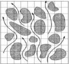
As discussed in the introduction, using the macroscopic upscaling (1-2), faithful simulations of the convective mass transfer in an aquifer often requires a high numerical resolution (e.g. [38, 37, 34]) because the characteristic length scale ($\lambda$) of the REV is typically at the order of $\Delta x$. As demonstrated schematically in Fig 1$(b)$, $\Delta x$ needs to be sufficiently small in order for $\lambda\rightarrow d$ so that computations on grid points would represent the actual mass transfer along streamlines. In the following two sections, a multiscale representation of the fine scale mass and momentum transfer has been studied, using the most robust volumetric mean of the time-averaged conservation laws [6, 10, 9, 48].

2.2 Multiscale intrinsic mass transfer model

The intrinsic space-time average is

$$\langle\overline{u}_{i}\rangle=\frac{1}{\Delta V_{f}}\int_{\Delta V}\overline{u}_{i}(x_{i},t)dV,$$

where $\Delta V_{f}$ is the volume of the fluid contained in a REV. Note the difference between $\langle\overline{u}_{i}\rangle^{v}$ and $\langle\overline{u}_{i}\rangle$, where $u_{D_{i}}=\phi\langle\overline{u}_{i}\rangle$ [22]. The time and volume averages are assumed to commute; i.e,. $\langle\overline{u}_{i}\rangle=\overline{\langle u_{i}\rangle},$ one may apply the temporal average into a volume averaged variable, and vice-versa. Using the intrinsic average $\langle\overline{\cdot}\rangle$, the space-time transmissivity in a REV may be resolved, which is neglected in the classical macroscopic model (1-2).

To illustrate the multiscale framework, we begin with the decomposition

$$u_{i}=u_{D_{i}}+u^{\prime}_{i}+u^{\prime\prime}_{i}$$

at three scales, where the first component, $u_{D_{i}}=\langle\overline{u}_{i}\rangle^{v}$, captures the mean discharge per unit area, but does not represent a details of the flow. The second component, $u^{\prime}_{i}$, adds the missing details into $u_{D_{i}}$ such that $\langle\overline{u^{\prime}}_{i}\rangle^{v}=0$ and $\langle\overline{u^{\prime}}_{i}\rangle\neq 0$. The third component, $u^{\prime\prime}_{i}$, represents a further details that satisfies $\langle\overline{u^{\prime\prime}}_{i}\rangle^{v}=0$ and $\langle\overline{u^{\prime\prime}}_{i}\rangle=0$. Clearly, the space-time mean intrinsic velocity $\langle\overline{u}_{i}\rangle=u_{D_{i}}+u_{i}^{\prime}$ resolves an additional details $u_{i}^{\prime}$ with respect to the classical mean Darcy velocity $u_{D_{i}}$. Similarly, the space-time intrinsic mean of the concentration of CO₂ can be obtained. In order to simplify the symbolic representation, $u_{i}$ is used for the dimensionless mean velocity $\langle\overline{u}_{i}\rangle$, and $c$ for the dimensionless mean concentration $\langle\overline{C}\rangle$ in the rest of this article, where all quantities are assumed uniform in the $x_{2}$ direction. Note that this two-dimensional assumption is an idealization for the radial symmetry of the dynamics of the CO₂ plume (e.g., [31, 37]), and has been adopted to aid the investigation on the proposed multiscale model development.

The derivation of the present intrinsic multiscale model for the mass transfer is similar to what was detailed by Breugem and Rees [10] for the heat transfer, and by Lage et al [25] for the momentum transfer (see also [6, 9, 48, 22, 30]). However, in the heat transfer model, an independent diffusion equation was considered in [10] to account for thermal conduction through the solid phase. In the present mass transfer model, the dissolution of the invaded phase has been parameterized through the averaging process. At a depth below $800$ m (see, [7]), the geothermal effects may be compensated by the geo-pressure gradient (see, [27] and chapter 2 of [14]), which is further illustrated by Pruess and Nordbotten [37]. The pressure gradient terms in eqs. (4-5) accounts for the geothermal pressure gradient. Since studies indicate a weak dependence between the molar volume of dissolved CO₂ and density of the binary mixture, the Boussinesq approximation is reasonable [5, 27, 14, 34]. Following the derivation of Lage et al [25], the macroscopic upscaling (1-2) has been replaced with the multiscale upscaling (3-6):

$$\frac{\partial u_{1}}{\partial x_{1}}+\frac{\partial u_{3}}{\partial x_{3}}=0$$ (3)

$$\frac{\partial u_{1}}{\partial t}+u_{1}\frac{\partial(u_{1}/\phi)}{\partial x_{1}}+u_{3}\frac{\partial(u_{1}/\phi)}{\partial x_{3}}=-\frac{\partial(P\phi)}{\partial x_{1}}+\frac{\alpha}{\mathcal{R}e}\nabla^{2}u_{1}-\frac{\phi u_{1}}{\mathcal{D}a\mathcal{R}e}$$ (4)

$$\frac{\partial u_{3}}{\partial t}+u_{1}\frac{\partial(u_{3}/\phi)}{\partial x_{1}}+u_{3}\frac{\partial(u_{3}/\phi)}{\partial x_{3}}=-\frac{\partial(P\phi)}{\partial x_{3}}+\frac{\alpha}{\mathcal{R}e}\nabla^{2}u_{3}-\frac{\phi u_{3}}{\mathcal{D}a\mathcal{R}e}+\frac{\mathcal{G}r}{\mathcal{R}e^{2}}c$$ (5)

$$\frac{\partial c}{\partial t}+u_{1}\frac{\partial c}{\partial x_{1}}+u_{3}\frac{\partial c}{\partial x_{3}}=-\frac{\mathcal{R}e^{2}}{\mathcal{G}r\mathcal{F}r^{2}}u_{3}+\frac{1}{\mathcal{R}e\mathcal{S}c}\nabla^{2}c.$$ (6)

In this model, the Schmidt number is $\mathcal{S}c=\frac{\nu}{D}$, the macroscopic Reynolds number and the Darcy number are defined by $\mathcal{R}e=\frac{\rho UH}{\mu}$ and $\mathcal{D}a=K/H^{2}$, respectively, where $\mathcal{R}e_{d}\ll\mathcal{R}e$ and $\mathcal{D}a=\mathcal{O}(1/\mathcal{R}e)$. Clearly, if $\mathcal{R}e\rightarrow\infty$, we have $\mathcal{D}a\rightarrow 0$, which corresponds to a macroscopic model (1-2).

As described in Appendix A, the space-time average of the nonlinear advection of momentum takes the form

$$\left\langle\overline{u_{j}\frac{\partial u_{i}}{\partial x_{j}}}\right\rangle=\langle\overline{u}_{j}\rangle\frac{\partial\langle\overline{u}_{i}\rangle}{\partial x_{j}}+\frac{\partial}{\partial x_{j}}\left(\overline{\langle u^{\prime\prime}_{i}\rangle\langle u^{\prime\prime}_{j}\rangle}+\langle\overline{u^{\prime\prime}_{i}u^{\prime\prime}_{j}}\rangle+\langle\overline{u}^{\prime\prime}_{i}\overline{u}^{\prime\prime}_{j}\rangle\right),$$

which resulted into the additional term

$$\frac{\partial}{\partial x_{j}}\left(\overline{\langle u^{\prime\prime}_{i}\rangle\langle u^{\prime\prime}_{j}\rangle}+\langle\overline{u^{\prime\prime}_{i}u^{\prime\prime}_{j}}\rangle+\langle\overline{u}^{\prime\prime}_{i}\overline{u}^{\prime\prime}_{j}\rangle\right),$$

of which, the first two components have been neglected in the present laminar mass transfer model, and the last term can be parameterized with the Brinkman model [11], which – in the dimensionless form – has taken the form of the second term on the right hand sides (rhs) of both (4) and (5). The third term on the rhs of (4, 5) has appeared due to the intrinsic average of the viscous and pressure stress, which models the density of the pressure drag and skin friction,

$$f_{i}=-\frac{\mu}{K}u_{D_{i}},$$

when the Reynolds number is small, i.e., $\mathcal{R}e_{d}=\mathcal{O}(1)$ [14].

Similarly, the nonlinear advection of the mass flux has resulted into the additional term

$$\frac{\partial}{\partial x_{j}}\left(\overline{\langle u^{\prime\prime}_{i}\rangle\langle c^{\prime\prime}_{j}\rangle}+\langle\overline{u^{\prime\prime}_{i}c^{\prime\prime}_{j}}\rangle+\langle\overline{u}^{\prime\prime}_{i}\overline{c}^{\prime\prime}_{j}\rangle\right)$$

of which the first two components have been neglected and the last component has been parameterized to model the effect of dissolution with the first term on the right hand side of (6).

2.3 The dissolution of CO₂ through the dispersive mass flux

Literature review does not indicate a common approach for modeling the effect CO₂ dissolution into the resident saline, despite there are few attempts (e.g. see [37]). If a CO₂ plume proceeds upward from an isolated source, the saline density at the interface increases by about $0.1$-$1\%$ [34]. To a first order approximation, the global density of the background environment adopts a vertically decreasing profile when the plume migrates upward, albeit more specific observational data would confirm the actual density profile (e.g. see also the density distribution presented by Pruess and Nordbotten [37]).

The present work has proposed a simple model

$$\frac{\partial}{\partial x_{j}}\langle\overline{u}^{\prime\prime}_{i}\overline{c}^{\prime\prime}_{j}\rangle=u_{3}\frac{\partial\tilde{c}}{\partial x_{3}}$$

for the mass dispersion associated with the microscopic space-time variation of mass and momentum, where a steady state horizontally homogeneous background concentration $\tilde{c}(x_{3})=C_{0}+\Gamma x_{3}$ has been assumed since the molecular mass of CO₂ is larger than that of brine (see [40, 20, 34]). With this model, one can define a Buoyancy frequency by $N^{2}_{b}=gM\Gamma/\rho_{0}$ to characterize the effect of dissolution, where $M$ is the molar mass of CO₂ and $\rho_{0}=C_{0}M$ is a reference density. Here, $N_{b}^{2}>0$ corresponds to a situation with $\Gamma>0$; i.e., in this case, CO₂ has been accumulated near the reservoir top, where the dissolution would result into gravitational fingers studied by Pau et al [34]. $N_{b}^{2}<0$ corresponds to $\Gamma<0$; i.e., CO₂ dissolution is now associated with a vertically migrating plume [12]. Accordingly, a Froude number is given by

$$\mathcal{F}r^{2}=\frac{U^{2}}{N^{2}_{b}H^{2}},$$

and using data from the Carrizo-Wilcox aquifer, Texas, e.g., $U\sim 5\times 10^{-5}\mathrm{m/s}$ and $H\sim 200~{}\mathrm{m}$ [37, 29], we estimate that $\mathcal{F}r\geq 1$ corresponds to $N_{b}\leq 2.5\times 10^{-7}~{}\mathrm{s^{-1}}$ and $\Gamma\geq-10^{-10}~{}\mathrm{M/m}$. Clearly, $\Gamma\ll-10^{-10}~{}\mathrm{M/m}$ results into $\mathcal{F}r\ll 1$, and the mass transfer analysis for varying $\mathcal{F}r$ exploits the effect of the CO₂ dissolution.

2.4 The natural convection mass transfer as a function of $\mathcal{F}r$

The dominant mechanism for the onset of background dissolution on the natural convection mass transfer during the migration of a CO₂ plume has now been studied with a dimensional analysis, which explains the effect of the variation of the Froude number. To estimate the order of magnitude of each term in the mass and momentum conservation laws (see Breugem and Rees [10]), consider the solutal Grashof number,

$$Gr=\frac{g\Delta\rho H^{3}}{\rho_{0}\nu^{2}}=\frac{g\beta\Delta cH^{3}}{\nu^{2}},$$

the Schmidt number, $Sc=\nu/D$, the horizontal length scale, $L$, and the vertical length scale, $H$. Note the large aspect ratio of typical aquifers (e.g. the Carrizo-Wilcox aquifer, Texas, US [29]) and the order of magnitude for the inertial term, $u_{1}\frac{\partial u_{1}}{\partial x_{1}}+u_{3}\frac{\partial u_{1}}{\partial x_{3}}=\mathcal{O}(\sqrt{\mathcal{G}r}H^{2}/L^{2})$. Using horizontal and vertical length scales, $L\sim 10~{}\mathrm{km}$ and $H\sim 200~{}\mathrm{m}$, respectively (e.g. [20]), where $H^{2}/L^{2}\ll 1$, as well as a fixed $Gr<2\,500$, and in the limit of $\mathcal{D}a\rightarrow\infty$, we obtain the following dimensionless linear system of PDEs

$$\frac{\partial u_{1}}{\partial x_{1}}+\frac{\partial u_{3}}{\partial x_{3}}=0,$$

$$0=-\frac{\partial p}{\partial x_{1}}+\frac{\partial^{2}u_{1}}{\partial x_{3}^{2}},$$

$$0=-\frac{\partial p}{\partial x_{3}}+c,$$

$$u_{3}=\frac{\partial^{2}c}{\partial x_{3}^{2}}.$$

The system is independent of the length and time scales, as well as of other dimensional parameters, and hence, exhibits a self-similar solution. The existence of a self similar solution indicates that the vertical length scale can be determined from the dimensional parameters $\nu$, $D$, $H$, $L$, and $N_{b}$ those appear in the dimensional system of equations. A dimensional reasoning can be used to define the vertical length scale as a function of the remaining other parameters; i.e.,

$$H^{6}=\frac{\nu DL^{2}}{N_{b}^{2}},$$

which gives an aspect ratio between the vertical scale and the horizontal scale:

$$\left(\frac{H}{L}\right)^{4}=\frac{Fr^{2}}{GrSc}.$$

Clearly, in the limit of $\mathcal{F}r\rightarrow\infty$ for a fixed $Gr$ and $Sc$, the vertical length scale extends to infinity; i.e., $H\rightarrow\infty$. This indicates that a non-zero gradient, $\Gamma$, tends to reduce vertical migration of the CO₂ plume. For too small a value of $\mathcal{F}r$, the vertical length scale is also too small; the plume will not continue to migrate vertically upward for small $\mathcal{F}r$. This dimensional analysis has a good agreement with the numerical simulations presented in section 4.3.2.

This section concludes by noting that the analysis of the multiscale model (3-6) with an adaptive wavelet multiscale technique is a novel contribution of the present research, in contrast to classical models, where the macroscopic model (1-2) analysed with a multiscale technique [34, 23, 31].

3 The adaptive wavelet multiscale simulation methodology

To outline the proposed numerical method, eqs (4-6) has been written in the following compact form:

$$\frac{\partial\Psi_{i}}{\partial t}+u_{j}\frac{\partial\Psi_{i}}{\partial x_{j}}=\frac{\partial R_{ij}}{\partial x_{j}}$$ (7)

where $\Psi_{i}$ represents $u_{1}$, $u_{3}$, or $c$, and $R_{ij}$ ($i,j=1,\,3$) represent the right hand sides of eqs (4-6). Since the velocity ($u_{1},u_{3}$) and the concentration ($c$) depends on each other simultaneously in a natural convection mass transfer application, a fully implicit time integration scheme has been adopted, where $u_{1}$, $u_{3}$, and $c$ are computed simultaneously.

3.1 Time integration

A fractional-step method, originally proposed by Chorin [13], has been applied to solve (7) for $\Psi_{i}^{n+1/2}$,

$$\frac{\Psi_{i}^{n+\frac{1}{2}}-\Psi_{i}^{n}}{\Delta t}+\frac{1}{2}\left(u_{j}^{n+\frac{1}{2}}\frac{\partial\Psi_{i}^{n+\frac{1}{2}}}{\partial x_{j}}+u_{j}^{n}\frac{\partial\Psi_{i}^{n}}{\partial x_{j}}\right)=\frac{1}{2}\left(R_{ij}^{n+\frac{1}{2}}+R_{ij}^{n}\right),$$

and it takes the following symbolic form

$$\mathcal{L}(\Psi_{i}^{n+\frac{1}{2}})=\bm{S}(\Psi_{i}^{n}),$$ (8)

where superscripts $n$ and $n+\frac{1}{2}$ mean the present time step and the first fraction of the next time step, respectively.

In the second fraction of a time step, eq. (3) is satisfied, $\frac{\partial u_{j}^{n+1}}{\partial x_{j}}=0$, such that the macroscopic model (1) is approximately diagnosed from

$$-\frac{\partial}{\partial x_{j}}\left(\frac{\partial(P\phi)^{n+1}}{\partial x_{j}}\right)=\frac{1}{\Delta t}\frac{\partial}{\partial x_{i}}\left(u_{D_{i}}^{n+1}\right),$$ (9)

where $u_{D_{i}}^{n+1}=u_{i}^{n+1}-u_{i}^{n+1/2}$. Setting $c^{n+1}=c^{n+\frac{1}{2}}$ from the nonlinear algebraic system (8), $u_{i}^{n+1}$ is also diagnosed from the elliptic problem (9), where (8) and (9) must be solved with efficient iterative solvers at each time step.

Since (8) is a nonlinear system, the classical Newton’s method

$$\Psi_{i}^{k+1,n+\frac{1}{2}}=\Psi_{i}^{k,n+\frac{1}{2}}+s_{k}$$

such that

$$\mathcal{J}s_{k}=\mathcal{S}(\Psi_{i}^{n})-\mathcal{L}\left(\Psi_{i}^{k,n+\frac{1}{2}}\right)$$

must evaluate the matrix-vector product $\mathcal{J}\bm{s}_{k}$ at every $k$-th iteration with $\mathcal{O}(\mathcal{N}^{2})$ operations, where $\mathcal{J}$ is the Jacobian matrix and $s_{k}$ is the error to be found. In order to reduce this high cost to $\mathcal{O}(\mathcal{N})$, let us consider the Frechet derivative

$$\mathcal{J}(\Psi_{i}^{k,n+\frac{1}{2}})s_{k}\approx\frac{\mathcal{L}(\Psi_{i}^{k,n+\frac{1}{2}}+\eta s_{k})-\mathcal{L}(\Psi_{i}^{k,n+\frac{1}{2}})}{\eta},$$

where $\eta$ is a small real number. The performance of this approach – known as the Jacobian free Newton-Krylov (JFNK) algorithm – was verified for multiphysics simulations. However, the improvement in the operation count is paid off by requiring a preconditioner, which is a serious drawback for extending the JFNK to the simulation of heat and mass transfer. In the present work, we study an alternative, where the multiscale wavelet method captures the multiscale physics, and the Newton’s method along with the Frechet derivative is used to reduce the residual of (8) by a certain fraction at each level of the present multiscale wavelet based solution methodology.

3.2 The multiscale wavelet methodology

The wavelet method (see [2, 28, 43]) captures the multiscale physics, using the best $\mathcal{N}$ terms of the multiscale decomposition

$$\Psi_{j}(x_{i})=\sum_{k}c_{2k}^{s}\varphi_{2k}^{s}(x_{i})+\sum_{l=s}^{\infty}\sum_{\eta=0}^{2^{d}-1}\sum_{k}d_{2k+1}^{\eta,l}\psi_{2k+1}^{\eta,l}(x_{i}),$$ (10)

according to a prescribed error tolerance $\epsilon$ on the magnitude of $d_{2k+1}^{\eta,s}$, where the error for resolving mass and/or energy is $\mathcal{O}(\epsilon)$. In (10), the first term represents a sampling of $\Psi_{j}$ ($u_{1}$, $u_{3}$, or $c$) on a coarse grid of $(2^{s}n+1)\times(2^{s}m+1)$ points, and the second term models the additional details of $\Psi_{j}$, which is not captured by the first term. In $2$D, with the exception of east and north boundaries, each coarse grid sampling $c_{2k}^{s}$ corresponds to three details data $d_{2k+1}^{\eta,s}$ (for $\eta=0,\,1,\,2$). For example, if the REV $[0,4]\times[0,2]$ is divided by a factor of $2$ in each direction, for the $2k\,$th vertex $(0,0)$, we have three $(2k+1)$ neighbors $(0,1)$, $(2,0)$, and $(2,1)$, where the corresponding detailed information is stored. When a REV is not sufficient to resolve $\Psi_{j}$ on the $2k$-th grid point, at least one $d_{2k+1}^{\eta,s}$ will have a magnitude larger than $\epsilon$, thereby providing with a natural framework for adapting the size of the REV to the local physical property. Therefore, one would begin with REVs on a coarse grid, perform a wavelet analysis, and recursively resize only those REVs, where wavelet coefficients are large. The wavelet transform may be computed with the Wavelet toolbox of Matlab without knowing the explicit information of $\varphi_{2k}^{s}$ and $\psi_{2k+1}^{\eta,s}$. Note that the grid adaptation is automatic with the wavelet method [44].

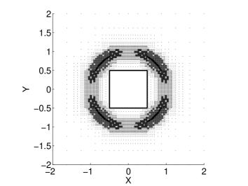
To illustrate the benefits of the multiscale wavelet representation, consider a prescribed concentration $c(x_{1},x_{3})$ that decays exponentially with respect to a circle of radius $1$. Taking the wavelet transform of $c(x_{1},x_{3})$, and recursively adapting the grid until all new wavelet coefficients satisfy a tolerance $\epsilon=10^{-4}$, an adaptive wavelet grid has been obtained, which is presented in Fig 2. Note that an obstacle of size $[-0.5,0.5]\times[-0.5,0.5]$ has been placed at the center of the domain, showing that the wavelet transform can be computed on complex domains.

Figure 2: An example of the wavelet based adaptive grid generation for a typical concentration field $c(x_{1},x_{3})$, where the ’box’ at the center of the domain represents an impermeable region. Each ’dot’ represents the physical position of a wavelet, representing a REV. More wavelets are used near a circle of radius $1$, where $c(x_{1},x_{3})$ has a sharp change, which confirms that REVs have been adapted to capture the local physical variation.

4 Results and verification

4.1 Verification results

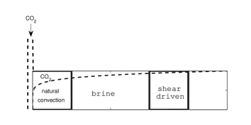
The shear driven or natural convection transport of CO₂ in an aquifer is an idealized model, and is useful for computational verification, where CO₂ moves horizontally just below the impermeable caprock, or vertically after it has been injected through an injection well. Adapted from [38, 32], a shear driven case and a natural convection case have been shown schematically in Fig 3. Note that the shear driven case has been chosen for the availability of reference data so that the numerical model can be quantified. In the next two simulations, the parameters $\mathcal{D}a=10^{4}$, $\mathcal{R}e=10^{3}$, $\alpha=1$, $\mathcal{S}c=0.72$, $\phi=90\%$ have been adapted from [48].

Figure 3: Schematic description for the distribution of the CO₂ phase after it has been injected into an aquifer. The natural convection mass transfer is an idealized model in the region that is next to the injection well - marked by the box. A region is marked “shear driven”, which may be a typical high permeability zone. Note that a shear driven case has been considered for the purpose of numerical verification only.

4.1.1 A shear driven mass transfer model for $\mathcal{G}r\rightarrow 0$

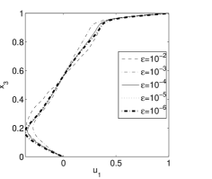
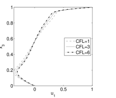
The shear driven mass transfer at $\mathcal{G}r=0$ is a benchmark example, where the momentum transfer is independent of the mass transfer. To study the performance of the proposed multiscale model, results of $30$ simulations of a shear driven mass transfer case with $\mathcal{G}r=0$ have now been summarized, where for each of the CFL numbers are $1$, $2$, $3$, $4$, $5$, $6$, the tolerance values are $\epsilon=10^{-6}$, $10^{-5}$, $10^{-4}$, $10^{-3}$, $10^{-2}$. In the present multiscale model, $\epsilon$ controls $\mathcal{N}$, as well as $\Delta x=\min(\Delta x_{1},\Delta x_{3})$ – the length scale of the smallest REV, where the grid points are adapted dynamically. To utilize the full advantage of this adaptivity, the maximum time step, $\Delta t$, has also been adapted dynamically based on CFL = $\Delta t/\Delta x$. Clearly, an increase of the CFL number (or $\epsilon$) would increase the global temporal (or spatial) error. These $30$ simulations provide an understanding of how the spatial and temporal errors are controlled globally in the present model. Note the use of a large CFL number (CFL=$6$) is a distinct feature of the present methodology, and is an important contribution to the field of computational heat and mass transfer.

$(a)$	$(b)$
$(c)$	$(d)$

Figure 4: Results from the performance studies of the proposed multiscale mode. The horizontal velocity $u=u_{1}\times\phi/U~{}\nicefrac{{m}}{{s}}$ as a function of $z=x_{3}\times H~{}\mathrm{m}$ along the vertical centerline of the aquifer. $(a)$ CFL $=3$ is fixed, but the tolerance, $\epsilon$, varies in the range $10^{-6}\leq\epsilon\leq 10^{-2}$. $(b)$ The tolerance $\epsilon=10^{-4}$ is fixed, but the CFL number varies in the range, $1\leq\hbox{CFL}\leq 6$. Clearly, the present model controls the space-time variation of the error, which is an important objective of this development. $(c)$ The number of degrees of freedom, $\mathcal{N}$, as a function of tolerance, $\epsilon$. The result for the present model, $\mathcal{N}\sim\epsilon^{-1/2}$, is compared with that of a classical finite difference (FD) model, $\mathcal{N}\sim\epsilon^{-1}$. $(d)$ Estimated boundary layer width, $\delta$, has been compared with $\mathcal{R}e^{-0.5}$ and $\mathcal{R}e^{-0.6}$.

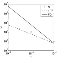
As demonstrated in Fig 4($a$-$b$), the variation of the spatial error tolerance $10^{-6}\leq\epsilon\leq 10^{-2}$ and the CFL number, $1\leq\hbox{CFL}\leq 6$ confirms the space-time error control of the proposed model. This velocity profile has a good agreement with the one, which was presented by Yang et al [48] and Guo and Zhao [19]. Fig 4($c$) shows that the computational degrees of freedom, $\mathcal{N}$, varies like $\epsilon^{-1/2}$, which means that $\mathcal{N}$ does not increase linearly if $\epsilon$ is decreased. Note that a direct numerical simulation of heat and mass transfer phenomena with a classical finite difference (FD) model, would increase $\mathcal{N}$ linear with a reduction of the error. The efficiency of the present model can be seen from the comparison in Fig 4($c$). Further more, with the error tolerance, $\epsilon=10^{-3}$, the present model needs $\mathcal{N}=3\,416$, which is about $5\%$ and $13\%$ of the grid points required by the simulations of Ghia et al [18] and Botella and Peyret [8], respectively. Although the physical setting of the present simulation is quite different than that of refs [18, 8], the similarity of dimensionless parameters allows us for a brief comparison in order to provide with a hint to the potential of the present model.

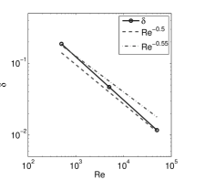
The laminar boundary layer thickness just below the top of the aquifer has been compared with the theoretical estimate, $\delta\sim\mathcal{R}e^{-1/2}$, in Fig 4($d$). A good fit between $\mathcal{R}e^{-0.5}$ and $\mathcal{R}e^{-0.6}$ indicates that the laminar boundary layer has been resolved more accurately at higher $\mathcal{R}e$. This idealized simulation at $\mathcal{G}r=0$ exploit the potential of the present model for simulating the best solution using the least number of the degrees of freedom, $\mathcal{N}$.

4.1.2 A natural convection case for $\mathcal{G}r\rightarrow\infty$

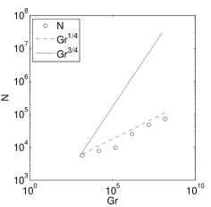
An idealization of the natural convection mass transfer in the aquifer has been simulated, where the boundary conditions, $C=1$ and $C=0$ on $x_{1}=0$ and $x_{1}=1$, represents the injection and removal of CO₂ across $x_{1}=0$ and $x_{1}=1$, respectively. Other boundary conditions are $\frac{\partial C}{\partial x_{3}}=0$ on $x_{3}=0$ and $x_{3}=1$, $\frac{\partial u_{1}}{\partial x_{1}}=0$ on $x_{1}=0$ and $x_{1}=1$. The velocity is assumed zero on all other boundaries. Under similar conditions, Nordbotten and Celia [32] studied mixed convection mass transfer in an aquifer, and showed that the migration of CO₂ occurs beneath the top boundary of the aquifer when natural convection dominates over the forced convection. Clearly, at large $\mathcal{G}r~{}(\rightarrow\infty)$, when the natural convection is dominant, the numerical simulation of the mass transfer in an aquifer would require high spatial resolution in order to resolve the solutal boundary layer. Hence, an estimate for $\mathcal{N}$ as a function of $\mathcal{G}r$ provides with a good understanding for the efficiency of the present multiscale model. Here, we summarize $7$ representative simulations with values of $\mathcal{G}r$ ($1.5\times 10^{3}$, $1.5\times 10^{4}$, $1.5\times 10^{5}$, $1.5\times 10^{6}$, $1.5\times 10^{7}$, $1.5\times 10^{8}$, and $1.5\times 10^{9}$), which show that $\mathcal{N}$ increases approximately as $\mathcal{G}r^{1/4}$. In Fig 5, this result is also compared with the estimate $\mathcal{G}r^{3/4}$ from the classical numerical simulation.

$(a)$	$(b)$

Figure 5: $(a)$ The number of degrees of freedom ($\mathcal{N}$) for resolving the multiscale mass transfer as a function of $\mathcal{G}r$ has been compared between the present multiscale model and a classical mass transfer model. The computational gain of a multiscale model at high $\mathcal{G}r$ is evident. $(b)$ The scaling of the CPU time with respect to $\mathcal{N}$, which shows that the CPU time remains approximately proportional to $\mathcal{N}$ for the entire period of simulation.

4.2 Simulation of a vertically migrating CO₂ plume

4.2.1 The Carrizo-Wilcox aquifer in Texas (CWT)

Over a period of $50$ years, the injection of approximately $370\times 10^{6}~{}\mathrm{m}^{3}$ super-critical CO₂ per year into the central section of the CWT would store about one fifth of the CO₂ emissions in Texas [29, 20]. The CWT formation is about $200~{}\mathrm{m}$ deep, and extends for a length of about $110~{}\mathrm{km}$ at an angle $\approx 1.5^{\hbox{\tiny{o}}}$ with the horizontal, reaching a depth of about $4~{}\mathrm{km}$ beneath the earth’s surface. A 2D vertical section of the CWT beneath a horizontal caprock at a depth of $3~{}\mathrm{km}$, which is $200~{}\mathrm{m}$ thick, and $2~{}\mathrm{km}$ long, has been simulated. The length to width aspect ratio of the model region is $10:1$, which is different than the actual aspect ratio of the CWT. The temperature of the aquifer is assumed at the initial value. A $400~{}\mathrm{m}$ wide CO₂ plume is assumed instantaneously at the center of the bottom boundary. The migration of CO₂ takes place under the action of gravity. Initially, both the resident brine and the invaded CO₂ are assumed at rest. The normal components of the gradient of mass and momentum fluxes are assumed zero on the lateral boundaries for all time.

Figure 6: Simulated plume migration and associated fingers in a $2,000~{}\mathrm{m}\times 200~{}\mathrm{m}$ domain. $(a)$ Distribution of CO₂ is marked with the dark color, where the light color represents brine. $(b)$ Distribution of grid points, showing that the most significant flow is located only in the region of fingers. $(c)$ The most significant flow occupies a part $400~{}\mathrm{m}\times 200~{}\mathrm{m}$ of the domain, where a high resolution is needed.

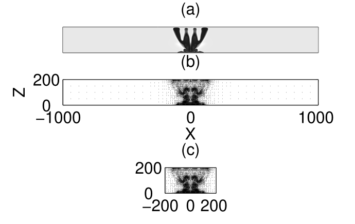
In Fig 6, simulated vertical migration of a CO₂ plume and the corresponding adapted grid points are presented at $t=11.4$ year. Clearly, the REVs have been adapted dynamically to resolve sharp gradients of the plume with respect to the error tolerance $\epsilon=10^{-4}$. The minimum size of a REV is given by $\Delta x_{1}\sim 2~{}\mathrm{m}$ and $\Delta x_{3}\sim 1.5~{}\mathrm{m}$ near the center of the plume, and the maximum size of the same is given by $\Delta x_{1}^{H}=62.5~{}\mathrm{m}$ and $\Delta x_{3}^{H}=50~{}\mathrm{m}$ away from the plume. The simulation needed an average $\mathcal{N}=3,593$ at each time step.

As depicted in Fig 6(c), the plume remains approximately in a region that extends from $-200~{}\mathrm{m}$ to $200~{}\mathrm{m}$ in the horizontal direction with respect to the center of the domain. However, only in this part of the domain, one might get the qualitatively equivalent results by solving the multiscale model (3-6) with a classical numerical method, using the uniform resolution of $\Delta x_{1}\sim 2~{}\mathrm{m}$ and $\Delta x_{3}\sim 1.5~{}\mathrm{m}$. In that case, at least $26,000$ grid points would be needed. In comparison to this estimate, the present methodology (with $\mathcal{N}\sim 3,593$) is about $86\%$ efficient, albeit a direct comparison with a previous simulation would be realistic.

4.2.2 A comparison of the computational gain with a TOUGH2 simulation

The recorded CPU time for the present simulation is approximately $2~{}\mathrm{ms~{}to}$ $3.6~{}\mathrm{ms}$ per grid point on a Dell T7400 workstation. A useful reference on the computational effort that is needed for a similar simulation is given by Pruess and Nordbotten [37], where the reported CPU time is about $700~{}\mathrm{ms}$ per grid block using the parallel code, TOUGH2, with $8$ processors in a Dell 5400 workstation. This is equivalent to about $5\,600~{}\mathrm{ms}$ per grid block for a single processor computation. The CPU time comparison with this particular TOUGH2 simulation exploits the advantage of $\mathcal{O}(\mathcal{N})$ computational complexity, which is one important development of the present multiscale model.

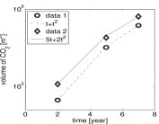
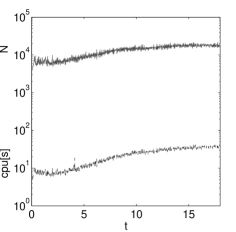
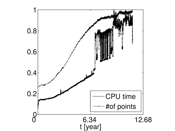
Since $\mathcal{N}$ varies at each time step due to adaptivity, we have recorded the CPU time for advancing the solution each time step, and two representative results are presented in Fig 5($b$) and Fig 7, showing that the CPU time is approximately proportional to $\mathcal{N}$. These results explore the promise of this development.

Figure 7: A scaling of the CPU time is compared with the number of grid points. In order to fit both the curves in the same frame, both the CPU time (upper curve) and the number of grid points (lower curve) have been normalized with respect to the maximum value of the corresponding data.

4.3 Analysis of natural convection mass transfer in an aquifer

4.3.1 Penetrative mass transfer

Ruckenstein [41] studied a generalized penetration theory for mass transfer in the vicinity of a fluid–fluid interface. In this section, we have briefly studied the multiscale nature of the penetrative mass transfer and the associated vorticity generation in a subsurface aquifer. In order to study the vorticity generation, we have simulated natural convection mass transfer at various values of $\phi$ and $\mathcal{D}a$.

In the limit of $\mathcal{D}a\rightarrow 0$, a first order estimate for the vorticity as a function of concentration is $\omega_{2}\sim\frac{\partial c}{\partial x_{1}}$, which indicates that a counter clockwise vorticity is generated in the region that is to the immediate left of the plume when the plume migrates upward [40]. Similarly, a clockwise vorticity is expected in the region that is to the immediate right of the plume. These clockwise and counter clockwise vortices interact with the porous structure, accelerate horizontal migration, and are responsible for transferring mass and momentum from one scale to the other. In Fig 8, the plume, the vorticity, and the adapted grid are presented for the porosities, $\phi=10\%$ and $\phi=20\%$, where $\mathcal{D}a=2.7\times 10^{-4}$. A complicated multiscale dynamics is observed. For the higher porosity, only $20\%$ of a REV is occupied by the fluid. A reduction of the porosity would decrease the volume of fluid faction in the REV, thereby strengthening the interaction between the fluid and the porous structure. For $\phi=10\%$, the mass transfer is accompanied with local sharp spatial gradients at multiple length scales, where $7,013$ grid points are needed because REVs are resized to resolve sharp gradients of the plume. If the porosity is doubled to $\phi=20\%$, the rate of mass transfer is enhanced by smoothing out the spatial gradients, and thus, the number of grid points is reduced to $3,553$. A better understanding of the vorticity field can be quantified with simulations at various values of $\mathcal{D}a$.

Figure 8: The effect of the porosity ($\phi$) in a natural convection mass transfer and the associated vorticity generation. $(a,\,b,\,c)$ $\phi=10\%$, $(d,\,e,\,f)$ $\phi=20\%$; $(a,d)$ the concentration of CO₂, red: CO₂, yellow: brine; $(b,e)$ the vorticity $\omega_{2}$ associated with the natural convection plume, red: counter clockwise vortex, blue: clockwise vortex, yellow: zero vorticity; $(c,f)$ the grid points. In $(c)$, $\mathcal{N}=7,013$, and in $(f)$, $\mathcal{N}=3,553$. Clearly, when $\phi$ increases the interaction between the fluid and the porous structure weakens.

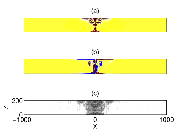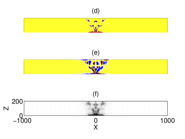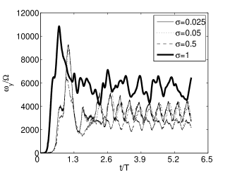
For the fixed $\phi=10\%$, let us present the time evolution for the mean vorticity for a variation of the Darcy number, $\mathcal{D}a=1.4\times 10^{-4},\,2.7\times 10^{-4},\,2.7\times 10^{-3},\,\hbox{and }5.4\times 10^{-3}$. Since the variation of $\mathcal{D}a$ is between $10^{-4}$ and $10^{-3}$, these simulations explore the sensitivity of perturbations introduced by the porous structure into the penetrative mass transfer. The growth of the mean vorticity, and its time evolution has been presented in Fig 9. Clearly, the Darcy number affects both the maximum of the mean vorticity and its amplitude of the fluctuation. Note that the natural convection mass transfer enhances the vorticity at the lowest of these values of $\mathcal{D}a$, which indicates that the penetrative mass transfer in a saline aquifer is accompanied with vorticity.

Figure 9: The time evolution of the mean vorticity $\frac{1}{A}\iint\omega_{2}(x_{1},x_{3},t)\,dA$, where $\omega_{2}=\frac{\partial u_{3}}{\partial x_{1}}-\frac{\partial u_{1}}{\partial x_{3}}$ is presented for $\mathcal{D}a=1.4\times 10^{-4},\,2.7\times 10^{-4},\,2.7\times 10^{-3},\,\hbox{and }5.4\times 10^{-3}$. The vorticity is normalized with respect to $\Omega=|\bm{\nabla}\times\bm{u}|$, and the time is normalized with respect to $T=L/U$, where $L$ and $U$ are length and velocity scales, respectively.

4.3.2 The effect of CO₂ dissolution into the natural convection mass transfer

$\mathcal{F}r=\infty$

$\mathcal{F}r=3.2$

$\mathcal{F}r=1.0$

Figure 10: Effect of dissolution on the vertical migration of a CO₂ plume for $\mathcal{F}r=\infty,\,3.2,\,1.0$ at $t=11.4~{}\mathrm{year}$. The red and yellow represents $c=1$ and $c=0$, respectively. The displayed region extends from $-600~{}\mathrm{m}$ to $600~{}\mathrm{m}$ horizontally, and from $0~{}\mathrm{m}$ to $200~{}\mathrm{m}$ vertically.

In the present model, the dissolution of CO₂ into the resident saline has been characterized by the Froude number $\mathcal{F}r$. In Fig 10, simulated distribution of CO₂ has been presented at $t=11.4~{}\mathrm{y}$ for three representative values of the Froude number, $\mathcal{F}r=\infty$, $3.3$, and $1$. The plume migrates vertically until it reaches the impermeable caprock at the top of the reservoir when $\mathcal{F}r=\infty$, when the brine is saturated with CO₂ such that $\Gamma=0$. When $1\leq\mathcal{F}r<\infty$, the plume migrates through a background environment with $\Gamma<0$. Comparing Fig 10(a) with Fig 10(c), we see that the plume has traveled less than half way in the vertical direction when $\mathcal{F}r=1$.

This simulation indicates a marked variability in the vertical migration of CO₂. These two-dimensional idealized simulations hint on the potential of the present model for analysing natural convection mass transfer and other related phenomena associated with CO₂ storage in aquifers. Further analysis with three dimensional simulations would be useful for explaining the multiscale and complex phenomena associated with the carbon capture and storage program.

5 Summary and discussion

5.1 Conclusion

This article introduces a multiscale modeling and simulation approach for the natural convection mass transfer in an aquifer. In order to tackle the challenges of multiscale phenomena, we have adopted the classical volume averaging technique to model a full details of the multiscale transport. Taking average heat and mass transfer with respect to a REV leads to a general framework for parameterizing the effect of multiscale phenomena which is not resolved with the averaging process. A wavelet based multiscale simulation methodology has been studied to dynamically resize the REV so that localized mass transfer can be resolved efficiently. A brief summary of the present development and key findings have been outlined below.

• Using the space-time average of the first principle conservation laws with respect to a representative elementary volume and a representative elementary time scale, this work has studied the governing equations so that heat, mass, and momentum transfer can be captured in a range of multiple length and time scales.

• Results from a set of $30$ representative numerical experiments at $\mathcal{G}r=0$ and $\mathcal{D}a=10^{4}$ show that the space-time error can be controlled with a priori prescribed error tolerance $\epsilon$ and CFL number. This a priori error control is an important contribution that would benefit future developments in the field of computational heat and mass transfer analysis.

• Simulations with an idealized natural convection mass transfer observes that the number of computational degrees of freedom varies like $\mathcal{N}\sim\mathcal{G}r^{1/4}$. Clearly, exploiting multiscale physics in the computational model has the potential to compute the most significant proportion of the flow using a near optimal computational effort. Further more, all simulations have indicated that the CPU time remains approximately proportional to $\mathcal{N}$, which means that the amount of computational work remains proportional to the amount of actual physical change in the system. To the author’s opinion, this property of the present model is a distinct feature with respect to classical approaches those are commonly used in the computational heat and mass transfer analysis.

• Present simulations with varying $\mathcal{F}r$ show a marked variation in the vertical migration of a CO₂ plume, i.e. the associated time scale, which suggests that the effect of dissolution of CO₂ in saline has a dominant role on the mass transfer mechanism. This would help to explain the dynamics of the subsurface CO₂ plume in various storage facilities.

• Present simulations observes that the vertical migration of a plume enhances the vorticity generation, where the dissolution of CO₂ has a strong influence on the vertical time scale of a plume.

• To the best of knowledge, this article, for the first time, has extended the second generation wavelet based adaptive technique to the field of subsurface flow and transport modeling. Hence, the present works adds a novel technology to the growing interests of multiscale modeling in the field of computational transport in aquifers.

5.2 Discussions

There are several possibilities to extend the present development. This includes the simulation of heat and mass transfer in a large aquifer – such as $110~{}\mathrm{km}$ long CWT or any other similar sites – where the phenomena is fully three-dimensional and gravitationally unstable. Future simulations, where the permeability, porosity, and other reservoir characteristics would have been obtained with advanced field technologies, may provide with an understanding of the degree to the proportion of actual multiscale features that can be resolved by the proposed model within the constraint of modern powerful computing resources. In a more realistic $3$D simulation, if $\mathcal{N}$ is still constrained by the computer power, then the smallest scale of a REV may need to be increased, where further improvements of the parameterization scheme would be necessary. Therefore, the present work leaves potential open questions those may be addressed in the future. However, the present research indicates that $3$D simulation will be benefited greatly if the present modeling approach is extended. Furthermore, the effect of variable permeability, temperature perturbation, and pathway transmissivities have not been examined in the present article. These works are currently underway.

Appendix A

The space-time double decomposition methodology

This section outlines the proposed model of resolving multiscale physics of a natural convection mass transfer when a plume migrates after CO₂ has been injected into an aquifer. The methodology aims to capture the average flow and transport with respect to a REV and a representative time scale for the REV, as well as to parameterize the effect of the unresolved flow. Researchers with interest in further mathematical details of the adopted double decomposition methodology may find the works of De Lemos [14] and Lage et al [25] useful. This section provides a brief outline for the decomposition of the inertia term $u_{j}\frac{\partial u_{i}}{\partial x_{j}}$ into a resolved proportion and an unresolved proportion, where the intrinsic space average ($\langle u_{i}\rangle$) is applied to time average ($\overline{u}_{i}$), and vice-versa (see also, section 2.2).

If we take the time average of a spatially averaged quantity, and use $\langle u^{\prime\prime}_{i}\rangle$ to denote temporal fluctuation of spatial averages, then a spatial mean may be decomposed as

$$\langle u_{i}\rangle=\langle\overline{u}_{i}\rangle+\langle u^{\prime\prime}_{i}\rangle,$$

where $\langle u^{\prime\prime}_{i}\rangle$ is the deviation of $\langle u_{i}\rangle$ with respect to the time average. The double decomposition is obtained by taking a spatial decomposition, $u_{i}=\langle u_{i}\rangle+\tilde{u}_{i}$, which is followed by a temporal decomposition; i.e.,

$$u_{i}=\underbrace{\langle\overline{u}_{i}\rangle+\langle u^{\prime\prime}_{i}\rangle}_{\langle u_{i}\rangle}+\overbrace{\overline{u}^{\prime\prime}_{i}+u^{\prime\prime}_{i}}^{\tilde{u}_{i}}$$

The following assumptions have been adopted to parameterize the effect of unresolved multiscale physics.

• $\rho_{0}\overline{\langle u^{\prime\prime}_{i}\rangle\langle u^{\prime\prime}_{j}\rangle}$ corresponds to momentum flux perturbation associated with the temporal fluctuations of the spatially averaged quantities $\langle u^{\prime\prime}_{i}\rangle$, which has been neglected. This term needs to be parameterized if a transition to turbulence is important; i.e., if $\mathcal{R}e_{p}\gg 1$.

• $\rho_{0}\langle\overline{u}^{\prime\prime}_{i}\overline{u}^{\prime\prime}_{j}\rangle$ corresponds to momentum diffusion associated with the temporal mean of spatial fluctuation (same as the spatial average of temporal fluctuation). In order to allow a smooth transition of flow and transport through pores of a porous medium, Brinkman [11] suggested to incorporate the effect of momentum diffusion. In the present work, this term has been parameterized to incorporate the effect of momentum diffusion.

• $\rho_{0}\overline{\langle u^{\prime\prime}_{i}u^{\prime\prime}_{j}\rangle}$ represents dispersion of momentum due to both time and spatial fluctuation, and can be neglected unless turbulence intermittency is important.

The above approximations, along with the conservation of mass and the Boussinesq approximation, leads to $u_{j}\frac{\partial u_{i}}{\partial x_{j}}=\frac{\partial u_{i}u_{j}}{\partial x_{j}}$, and hence, the spatio-temporal average of the divergence of the momentum flux (divided by the density) can be derived recursively. First, let us apply the spatial decomposition, $u_{i}=\langle u_{i}\rangle+\tilde{u}_{i}$, and write

$$\frac{\partial}{\partial x_{j}}\overline{\langle u_{i}u_{j}\rangle}=\frac{\partial}{\partial x_{j}}\overline{[\langle u_{i}\rangle\langle u_{j}\rangle+\langle\tilde{u}_{i}\tilde{u}_{j}\rangle]}$$

Second, both the mean, $\langle u_{i}\rangle$ and the fluctuation, $\tilde{u}_{i}$, are decomposed into a temporal mean and fluctuation, and as a result,

$$\frac{\partial}{\partial x_{j}}\overline{\langle u_{i}u_{j}\rangle}=\frac{\partial}{\partial x_{j}}[\langle\overline{u}_{i}\rangle\langle\overline{u}_{j}\rangle+\overline{\langle u^{\prime\prime}_{i}\rangle\langle u^{\prime\prime}_{j}\rangle}+\langle\overline{\tilde{u}_{i}\tilde{u}_{j}}\rangle]$$

Third, the decomposition of the spatial fluctuation, $\tilde{u}_{i}$ into a temporal mean, $\overline{u}^{\prime\prime}_{i}$, and a temporal fluctuation, $u^{\prime\prime}_{i}$, (i.e. $\tilde{u}_{i}=\overline{u}^{\prime\prime}_{i}+u^{\prime\prime}_{i}$) results into the final form

$$\frac{\partial}{\partial x_{j}}\overline{\langle u_{i}u_{j}\rangle}=\frac{\partial}{\partial x_{j}}[\langle\overline{u}_{i}\rangle\langle\overline{u}_{j}\rangle+\overline{\langle u^{\prime\prime}_{i}\rangle\langle u^{\prime\prime}_{j}\rangle}+\langle\overline{u}^{\prime\prime}_{i}\overline{u}^{\prime\prime}_{j}\rangle]+\overline{\langle u^{\prime\prime}_{i}u^{\prime\prime}_{j}\rangle}].$$

Finally, using the average mass conservation,

$$\frac{\partial}{\partial x_{j}}\overline{\langle u_{i}u_{j}\rangle}=\langle\overline{u}_{j}\rangle\frac{\partial\langle\overline{u}_{i}\rangle}{\partial x_{j}}+\frac{\partial}{\partial x_{j}}[\overline{\langle u^{\prime\prime}_{i}\rangle\langle u^{\prime\prime}_{j}\rangle}+\overline{\langle u^{\prime\prime}_{i}u^{\prime\prime}_{j}\rangle}+\langle\overline{u}^{\prime\prime}_{i}\overline{u}^{\prime\prime}_{j}\rangle].$$

Note that the above decomposition tells us what physical features of the problem has been modelled and the assumptions made to neglect some of the other physics. Similar approach has been used to derive Eq (6).

References

- Alam and Islam [2014] Alam J, Islam MR (2014) A multiscale eddy simulation methodology for the atmospheric ekman boundary layer. Geophysical & Astrophysical Fluid Dynamics 0(0):1–20, DOI 10.1080/03091929.2014.975127, in press
- Alam et al [2012] Alam JM, Kevlahan NKR, Vasilyev OV, Hossain Z (2012) A multi-resolution model for the simulation of transient heat and mass transfer. Numerical Heat Transfer, Part B 61:1–24
- Alam et al [2014] Alam JM, Walsh RP, Alamgir Hossain M, Rose AM (2014) A computational methodology for two-dimensional fluid flows. International Journal for Numerical Methods in Fluids 75(12):835–859
- Bachu et al [1994] Bachu S, Gunter W, Perkins E (1994) Aquifer disposal of CO2: Hydrodynamic and mineral trapping. Energy Conversion and Management 35(4):269 – 279
- Barbero et al [1983] Barbero J, Hepler L, McCurdy K, Tremaine P (1983) Thermodynamics of aqueous carbon dioxide and sulfur dioxide: Heat capacities, volumes, and the temperature dependence of ionization. Can J Chem 61(11):2509–2519
- Bear [1972] Bear J (1972) Dynamics of fluids in porous media. Elsevier (New York)
- Benson and Cook [2005] Benson SM, Cook P (2005) Underground Geological Storage, IPCC Special Report on Carbon Dioxide Capture and Storage, Intergovernmental Panel on Climate Change, Cambridge University Press, Cambridge, U.K., chap 5, pp 195–276
- Botella and Peyret [1998] Botella O, Peyret R (1998) Benchmark spectral results on the lid-driven cavity flow. Computers & Fluids 27(4):421 – 433
- Braga and de Lemos [2009] Braga EJ, de Lemos MJ (2009) Laminar and turbulent free convection in a composite enclosure. International Journal of Heat and Mass Transfer 52(3 4):588 – 596
- Breugem and Rees [2006] Breugem W, Rees D (2006) A derivation of the volume-averaged boussinesq equations for flow in porous media with viscous dissipation. Transport in Porous Media 63(1):1–12
- Brinkman [1949] Brinkman H (1949) A calculation of the viscous force exerted by a flowing fluid on a dense swarm of particles. Applied Scientific Research 1(1):27–34
- Chadwick et al [2009] Chadwick R, Noy D, Arts R, Eiken O (2009) Latest time-lapse seismic data from sleipner yield new insights into CO2 plume development. Energy Procedia 1(1):2103 – 2110
- Chorin [1968] Chorin A (1968) Numerical solution of navier-stokes equation. Math Commp 22:745–762
- De Lemos [2006] De Lemos M (2006) Turbulence in Porous Media: Modeling And Applications. Chemical, Petrochemical & Process, Elsevier Science Limited
- Elenius and Johannsen [2012] Elenius M, Johannsen K (2012) On the time scales of nonlinear instability in miscible displacement porous media flow. Computational Geosciences 16:901–911
- Farajzadeh et al [2007] Farajzadeh R, Salimi H, Zitha PL, Bruining H (2007) Numerical simulation of density-driven natural convection in porous media with application for CO2 injection projects. International Journal of Heat and Mass Transfer 50(25 26):5054 – 5064
- Farajzadeh et al [2009] Farajzadeh R, Zitha PLJ, Bruining J (2009) Enhanced mass transfer of CO2 into water: Experiment and modeling. Industrial & Engineering Chemistry Research 48(13):6423–6431
- Ghia et al [1982] Ghia U, Ghia K, Shin C (1982) High-Re solutions for incompressible flow using the navier-stokes equations and a multigrid method. Journal of Computational Physics 48(3):387–411
- Guo and Zhao [2002] Guo Z, Zhao TS (2002) Lattice Boltzmann model for incompressible flows through porous media. Physical Review E 66(3):036,304–9
- Hesse et al [2008] Hesse MA, Orr FM, Tchelepi HA (2008) Gravity currents with residual trapping. Journal of Fluid Mechanics 611:35–60
- Homsy [1987] Homsy GM (1987) Viscous fingering in porous media. Annual Review of Fluid Mechanics 19(1):271–311
- Hsu and Cheng [1990] Hsu C, Cheng P (1990) Thermal dispersion in a porous medium. International Journal of Heat and Mass Transfer 33(8):1587 – 1597
- Jenny et al [2006] Jenny P, Lee S, Tchelepi H (2006) Adaptive fully implicit multi-scale finite-volume method for multi-phase flow and transport in heterogeneous porous media. Journal of Computational Physics 217(2):627 – 641
- Künze et al [2013] Künze R, Lunati I, Lee SH (2013) A multilevel multiscale finite-volume method. Journal of Computational Physics 255(0):502 – 520
- Lage et al [2002] Lage JL, de Lemos MJS, Nield DA (2002) Modeling turbulence in porous media. Transport phenomena in porous media 2:198–230
- Leetaru et al [2009] Leetaru HE, Frailey SM, Damico J, Mehnert E, Birkholzer J, Zhou Q, Jordan PD (2009) Understanding CO2 plume behavior and basin-scale pressure changes during sequestration projects through the use of reservoir fluid modeling. Energy Procedia 1(1):1799 – 1806
- Lindeberg and Wessel-Berg [1997] Lindeberg E, Wessel-Berg D (1997) Vertical convection in an aquifer column under a gas cap of CO2. Energy Conversion and Management 38, Supplement(0):S229 – S234
- Mallat [1999] Mallat S (1999) A wavelet tour of signal processing. Academic Press, New York
- Nicot [2008] Nicot JP (2008) Evaluation of large-scale CO2 storage on fresh-water sections of aquifers: An example from the Texas Gulf coast basin. International Journal of Greenhouse Gas Control 2(4):582 – 593
- Nithiarasu et al [1999] Nithiarasu P, Seetharamu K, Sundararajan T (1999) Numerical investigation of buoyancy driven flow in a fluid saturated non-darcian porous medium. International Journal of Heat and Mass Transfer 42(7):1205 – 1215
- Nordbotten [2009] Nordbotten J (2009) Adaptive variational multiscale methods for multiphase flow in porous media. Multiscale Modeling & Simulation 7(3):1455–1473
- Nordbotten and Celia [2006] Nordbotten JM, Celia MA (2006) Similarity solutions for fluid injection into confined aquifers. Journal of Fluid Mechanics 561:307–327
- Nordbotten et al [2005] Nordbotten JM, Celia MA, Bachu S (2005) Injection and storage of CO2 in deep saline aquifers: Analytical solution for CO2 plume evolution during injection. Transport in Porous Media 58:339–360
- Pau et al [2010] Pau GS, Bell JB, Pruess K, Almgren AS, Lijewski MJ, Zhang K (2010) High-resolution simulation and characterization of density-driven flow in CO2 storage in saline aquifers. Advances in Water Resources 33(4):443 – 455
- Peaceman and Rachford [1962] Peaceman DW, Rachford HH (1962) Numerical calculation of the multidimensional miscible displacement. Society of Petroleum Engineering Journal 2:327–339
- Popiolek and Awruch [2009] Popiolek T, Awruch A (2009) An adaptive mesh strategy for transient flows simulations. In: Computational Modeling (MCSUL), 2009 Third Southern Conference on, pp 71 –76
- Pruess and Nordbotten [2011] Pruess K, Nordbotten J (2011) Numerical simulation studies of the long-term evolution of a CO2 plume in a saline aquifer with a sloping caprock. Transport in Porous Media 90:135–151
- Pruess and Zhang [2008] Pruess K, Zhang K (2008) Numerical modeling studies of the dissolution diffusion convection process during CO2 storage in saline aquifers. Tech. Rep. LBNL-1243E, Lawrence Berkeley National Laboratory, California
- Riaz and Meiburg [2003] Riaz A, Meiburg E (2003) Three-dimensional miscible displacement simulations in homogeneous porous media with gravity override. Journal of Fluid Mechanics 494:95–117
- Riaz et al [2006] Riaz A, Hesse M, Tchelepi HA, Orr FM (2006) Onset of convection in a gravitationally unstable diffusive boundary layer in porous media. Journal of Fluid Mechanics 548:87–111
- Ruckenstein [1968] Ruckenstein E (1968) A generalized penetration theory for unsteady convective mass transfer. Chemical Engineering Science 23(4):363 – 371
- Straughan [2008] Straughan B (2008) Convection in porous media. In: Stability and Wave Motion in Porous Media, Applied Mathematical Sciences, vol 165, Springer New York, pp 1–45
- Sweldens [1997] Sweldens W (1997) The lifting scheme: A construction of second generation wavelets. SIAM J Math Anal 29(2):511–546
- Vasilyev and Kevlahan [2005] Vasilyev OV, Kevlahan NR (2005) An adaptive multilevel wavelet collocation method for elliptic problems. J Comput Phys 206:412–431
- Whitaker [1999] Whitaker S (1999) The Method of Volume Averaging. Springer
- Wirasaet and Paolucci [2005] Wirasaet D, Paolucci S (2005) Application of an adaptive wavelet method to natural-convection flow in a differentially heated cavity. ASME Conference Proceedings 2005(47330):499–511
- Wirasaet and Paolucci [2006] Wirasaet D, Paolucci S (2006) The application of an adaptive wavelet method to the 3-d natural-convection flow in a differentially heated cavity. ASME Conference Proceedings 2006(47861):581–592
- Yang et al [2012] Yang D, Xue Z, Mathias SA (2012) Analysis of momentum transfer in a lid-driven cavity containing a Brinkman-Forchheimer medium. Transport in Porous Media 92:101–118