On the joint analysis of CMB temperature and lensing-reconstruction power spectra

Abstract

Gravitational lensing provides a significant source of cosmological information in modern CMB parameter analyses. It is measured in both the power spectrum and trispectrum of the temperature fluctuations. These observables are often treated as independent, although as they are both determined from the same map this is impossible. In this paper, we perform a rigorous analysis of the covariance between lensing power spectrum and trispectrum analyses. We find two dominant contributions coming from: (i) correlations between the disconnected noise bias in the trispectrum measurement and sample variance in the temperature power spectrum; and (ii) sample variance of the lenses themselves. The former is naturally removed when the dominant $N^{(0)}$ Gaussian bias in the reconstructed deflection spectrum is dealt with via a partially data-dependent correction, as advocated elsewhere for other reasons. The remaining lens-cosmic-variance contribution is easily modeled but can safely be ignored for a Planck-like experiment, justifying treating the two observable spectra as independent. We also test simple likelihood approximations for the deflection power spectrum, finding that a Gaussian with a parameter-independent covariance performs well.

I Introduction

Weak gravitational lensing by large-scale structure leaves subtle imprints in the temperature anisotropies of the cosmic microwave background (CMB); see Lewis and Challinor (2006) for a review. These imprints can be detected in surveys with resolution better than a few arcminutes and used to reconstruct the lensing deflection field Zaldarriaga and Seljak (1999); Hu (2001a). Since the lensing deflections depend on the growth of structure and geometry at much lower redshifts ($z\sim 2$) than the CMB last-scattering surface, lens reconstructions can be used to constrain parameters that are largely degenerate in the primary anisotropies sourced at last-scattering. Examples include sub-eV neutrino masses, spatial curvature, dark energy and modifications to gravity (e.g. Hu (2002); Kaplinghat et al. (2003); Verde and Spergel (2002); Acquaviva et al. (2004); Calabrese et al. (2008); Hall and Challinor (2012)).

Lensing is an emerging frontier of observational cosmology. The first direct measurements of the deflection power spectrum were reported recently by the ACT Das et al. (2011, 2013), SPT van Engelen et al. (2012) and Planck Planck Collaboration et al. (2013a) teams with significances of $4.6$, $6.3$ and $25\,\sigma$, respectively. These measurements provide the first evidence for dark energy from the CMB alone. Since lens reconstructions are quadratic in the temperature anisotropies, the power spectrum of the reconstruction is probing the 4-point non-Gaussianity of the CMB induced by lensing Hu (2001b). The statistical power of lens reconstructions is expected to improve rapidly with ongoing analyses of the full $2500\,\mathrm{deg}^{2}$ SPT survey and the full-mission data from Planck, which also allow for polarization-based lensing reconstruction. Lensing also affects the power spectrum (or 2-point function) of the temperature anisotropies, smoothing the acoustic peaks and transferring power from large to small scales (e.g. Seljak (1996)). The smoothing effect has been detected at nearly $10\,\sigma$ in current temperature power spectrum measurements Story et al. (2012); Planck Collaboration et al. (2013b).

A question that has received only limited attention to date is how one should model the likelihood of the lensed CMB anisotropies when deriving constraints on cosmological parameters. As the unlensed CMB and deflection field can be approximated as Gaussian on the scales relevant for CMB lensing, it is straightforward to write down a formal expression for the likelihood of the lensed temperature Hirata and Seljak (2003). However, this is very difficult to work with directly. Indeed, working with the exact likelihood even for Gaussian fields in mega-pixel maps is computationally prohibitive. Instead, in the Gaussian case, at high multipoles the data is usually compressed to an empirical power spectrum (or set of cross-spectra) and an approximate likelihood is constructed based on this spectrum and its covariance. Such an approach is both computationally feasible and allows for robust treatment of instrumental effects such as beam asymmetry. For non-Gaussian fields, like the lensed CMB, working with only the empirical power spectrum is clearly lossy. Instead, we should include further empirical connected $n$-point functions in our compressed data. In the context of CMB lensing, the 4-point function is the most relevant moment and the information it carries is captured in the estimated power spectrum of the reconstructed deflection field.

Parameter analyses involving lens reconstruction to date have followed the route described above. However, they have simply combined estimates of the temperature power spectrum and the lensing power spectrum as if they were independent Sherwin et al. (2011); van Engelen et al. (2012); Planck Collaboration et al. (2013a). Since both power spectra are derived from the same CMB temperature map, one might question the validity of this approach, raising the concern that lensing information is inadvertently being double counted. While early lensing forecasts Hu (2002); Kaplinghat et al. (2003); Lesgourgues et al. (2006) addressed this by using unlensed CMB power spectra, an optimal combination of the observed lensed CMB 2- and 4-point functions should model their cross-covariance. Intuitively, we might expect two effects to be relevant. First, the statistical noise in the reconstruction, due to chance alignments in the unlensed CMB which mimic the locally-anisotropic effects of lensing, is dependent on the CMB fluctuations themselves. If, due to cosmic variance, the unlensed temperature anisotropies fluctuate high at some particular scale, the noise in the lens reconstruction will also fluctuate high. The mode-coupling nature of lens reconstruction, whereby modes near the resolution limit of the observation dominate the reconstruction on much larger scales, will lead to broad correlations between the temperature and lensing power spectra. Since the reconstruction is quadratic, the correlation of the power spectra involves the CMB 6-point function, the disconnected part of which arises from the effect just decribed. The second effect is due to the cosmic variance of the lenses. If the lensing field fluctuates high at some scale, the reconstructed power will also fluctuate high at the same scale. In parallel, there will be more smoothing of the acoustic peaks in the measured CMB power spectrum giving an anti-correlation with the reconstucted lensing power at the location of acoustic peaks and a positive correlation at troughs. This effect is second order in the deflection power and derives from the connected part of the CMB 6-point function. As we shall show, the induced correlations are rather small (a few percent) for a Planck-like experiment for broad-band measures of the lensing power such as a lensing power spectrum amplitude. Essentially, this is because there are a limited number of modes of the lensing power spectrum that influence the acoustic part of the temperature power spectrum, and the correlation due to cosmic variance of these modes is diluted by the significant noise due to cosmic variance of the CMB and instrumental noise (i.e. the fact that lensing measurements from the CMB 2- and 4-point function are not limited by cosmic variance of the lenses). Moreover, the first effect mentioned above produces rather small lensing amplitude correlations since CMB modes at different scales fluctuate independently, and most of the information on peak smearing in the CMB power spectrum comes from modes near the acoustic peaks and troughs, whereas the reconstruction of (large-scale) lenses is most effective at CMB scales where the CMB spectrum changes most rapidly, i.e. between acoustic peaks and troughs. Note also that even the unlensed CMB anisotropies are correlated with the lensing field due to the late-time integrated Sachs-Wolfe effect Goldberg and Spergel (1999). This mostly produces a diagonal covariance between the power spectra of the lens reconstruction and the lensed CMB which falls rapidly at small scales ($L>100$). One of our main aims in this paper is to quantify these arguments with detailed calculations of the 6-point function, verified with simulations, and to assess whether the correlations are small enough to be safely ignored in the likelihood.

A further issue concerns the form of the likelihood for the power spectrum estimates. This has been well studied for Gaussian fields, e.g. Bond et al. (2000); Verde et al. (2003); Smith et al. (2006a); Hamimeche and Lewis (2008), and simple approximate forms are known to give reliable parameter constraints when applied on all but the largest scales. However, the lensing reconstruction is quadratic in the nearly Gaussian CMB fluctuations and therefore highly non-Gaussian. Here, we test a particularly simple form of the lensing power likelihood, a Gaussian with model-independent covariance. Constraining the amplitude and tilt of a fiducial deflection power spectrum, we demonstrate that the fiducial-Gaussian approximation performs well, returning maximum-likelihood points that scatter across simulations in a manner consistent with the width of the likelihood.

The paper is organised as follows. We review CMB lensing reconstruction in Sec. II and we describe our simulations of lensed CMB maps and the mechanics of our reconstructions in Sec. III. Section IV surveys known results for the auto-correlations of the lensed CMB temperature power spectrum and the reconstruction power spectrum. In Sec. V we present results for the cross-correlation of these power spectra and assess the importance of correlations for estimating cosmological parameters. We test likelihood approximations for the lensing reconstruction (in isolation) in Sec. VI and conclude in Sec. VII. In Appendix A we provide intuitive arguments for the magnitude of the temperature-lensing power correlation. A series of further appendices provide calculational details, and motivate some of the approaches taken in the main text. Table 1 summarises the key quantities, and their definitions and symbols, used in this paper.

Symbol		Description		Definition
$T$		Unlensed CMB temperature		Eq. (1)
$\tilde{T}$		Lensed CMB temperature		Eq. (1)
$\phi_{\text{in}}$		Input lensing potential field in simulations
$\hat{\phi}$		Lensing reconstruction (quadratic in $\tilde{T}$)		Eq. (9)
$A_{L}$, $\tilde{g}$		Normalisation and weights for $\hat{\phi}$		Eqs. (10), (11)
$C^{XX}_{l}$		Fiducial theoretical power spectrum of $X=T$, $\tilde{T}$ or $\phi$ (without noise/beam)
$C^{\tilde{T}\tilde{T}}_{l,\mathrm{expt}}$		Lensed temperature power spectrum including beam-deconvolved noise		Eq. (18)
$\hat{C}^{XX}_{l}$		Empirical power spectrum of a realisation of $X=T$, $\tilde{T}$, $\phi_{\text{in}}$ or $\hat{\phi}$		Eq. (19)
$N^{(0)}_{l}$		Gaussian, fully disconnected noise bias of $\hat{C}^{\hat{\phi}\hat{\phi}}_{l}$		Eq. (16)
$N^{(1)}_{l}$, $N^{(2)}_{l}$		Biases of $\hat{C}^{\hat{\phi}\hat{\phi}}_{l}$ at $\mathcal{O}(C^{\phi\phi})$ and $\mathcal{O}[(C^{\phi\phi})^{2}]$		Ref. Hanson et al. (2011)
$\hat{N}^{(0)}_{l}$		Data-dependent, empirical bias subtraction term		Eqs. (17), (32)
$\mathrm{cov}(\hat{C}^{\hat{\phi}\hat{\phi}}_{L},\hat{C}^{\tilde{T}\tilde{T}}_{L^{\prime},\mathrm{expt}})$		Covariance of CMB temperature and lensing reconstruction power spectra		Eq. (33)
$\mathrm{cov}(\hat{C}^{\hat{\phi}\hat{\phi}}_{L},\hat{C}^{\tilde{T}\tilde{T}}_{L^{\prime},\mathrm{expt}})_{\text{disconn.}}$		Noise contribution (from Gaussian, fully disconnected CMB 6-point function)		Eqs. (35), (36)
$\mathrm{cov}(\hat{C}^{\hat{\phi}\hat{\phi}}_{L},\hat{C}^{\tilde{T}\tilde{T}}_{L^{\prime},\mathrm{expt}})^{\text{conn.4pt.}X}_{\text{[(non-)primary]}}$		Trispectrum contributions of type $X=A,B$ [from (non-)primary coupling]		Appendix D
$\mathrm{cov}(\hat{C}^{\hat{\phi}\hat{\phi}}_{L},\hat{C}^{\tilde{T}\tilde{T}}_{L^{\prime},\mathrm{expt}})_{\langle\tilde{T}_{1}\cdots\tilde{T}_{6}\rangle_{c,\mathrm{dom.}}^{(4)}}$		Matter cosmic variance contribution [from $\mathcal{O}(\phi^{4})$ connected CMB 6-point function]		Eqs. (45), (111)
$A$		Overall lensing amplitude of a fiducial lensing power spectrum		$C^{\phi\phi}_{l}$$=$$AC^{\phi\phi}_{l}|_{\text{fid}}$
$\hat{A}$		Estimator for $A$ based on reconstruction power spectrum, i.e. CMB trispectrum		Eq. (54)
$\hat{A}^{\prime}$		Estimator for $A$ based on CMB power spectrum		Eq. (55)
$n$		Tilt of a fiducial lensing power spectrum $C^{\phi\phi}_{l}|_{\text{fid}}$		Eq. (66)

Table 1: Summary of the main quantities used throughout this paper (roughly ordered after first appearance).

II CMB lensing reconstruction

The lensed CMB temperature $\tilde{T}({\hat{\mathbf{n}}})$ along direction ${\hat{\mathbf{n}}}$ is related to the unlensed temperature $T({\hat{\mathbf{n}}})$ by the deflection field $\mathbf{\alpha}(\hat{\mathbf{n}})$

$$\tilde{T}(\hat{\mathbf{n}})=T[\hat{\mathbf{n}}+\mathbf{\alpha}(\hat{\mathbf{n}})].$$ (1)

The deflection angle can be written in the Born approximation as the angular gradient of a lensing potential, $\mathbf{\alpha}({\hat{\mathbf{n}}})=\mathbf{\nabla}\phi(\hat{\mathbf{n}})$, which is given by an integral along the (unperturbed) line of sight of the gravitational potentials (e.g. Lewis and Challinor (2006)).

On the full sky, the effect of lensing on the CMB temperature can be expressed perturbatively by Taylor expanding Eq. (1). Expanding in spherical harmonics, the multipoles of the lensed CMB, $\tilde{T}_{lm}$, are related to those of the unlensed CMB $T_{lm}$ and the lensing potential $\phi_{lm}$ via Hu (2000)

$$\tilde{T}_{lm}=T_{lm}+\delta T_{lm}+\delta^{2}T_{lm}+\cdots,$$ (2)

where changes due to lensing $\delta^{n}T_{lm}$ are of order $\mathcal{O}(\phi^{n})$ and linear in the unlensed temperature $T$:

$$\delta T_{lm} = \sum_{\underline{l}_{1},\underline{l}_{2}}\phi_{\underline{l}_{1}}T_{\underline{l}_{2}}I^{mm_{1}m_{2}}_{ll_{1}l_{2}},$$ (3)

$$\delta^{2}T_{lm} = \sum_{\underline{l}_{1},\underline{l}_{2},\underline{l}_{3}}\phi_{\underline{l}_{1}}\phi_{\underline{l}_{2}}T_{\underline{l}_{3}}J^{mm_{1}m_{2}m_{3}}_{ll_{1}l_{2}l_{3}},$$ (4)

where we have introduced the notation $\underline{l}\equiv(lm)$ and $I$ denotes an angular integral over a product of (derivatives of) spherical harmonics given by Hu (2000)

$$I^{mm_{1}m_{2}}_{ll_{1}l_{2}} = (-1)^{m}\left(\begin{matrix}l&l_{1}&l_{2}\\ -m&m_{1}&m_{2}\end{matrix}\right)F_{ll_{1}l_{2}}.$$ (5)

Expressions for $J^{mm_{1}m_{2}m_{3}}_{ll_{1}l_{2}l_{3}}$ can be found in Hanson et al. (2011). The geometrical factor $F_{l_{1}Ll_{2}}$, which is symmetric in the last two indices, is given by

$$F_{l_{1}Ll_{2}}=\left[L(L+1)-l_{1}(l_{1}+1)+l_{2}(l_{2}+1)\right]\sqrt{\frac{(2l_{1}+1)(2L+1)(2l_{2}+1)}{16\pi}}\left(\begin{matrix}l_{1}&L&l_{2}\\ 0&0&0\end{matrix}\right),$$ (6)

and describes the rotationally-invariant part of the coupling between the three multipoles.

It is possible to reconstruct the lensing potential $\phi(\hat{\mathbf{n}})$ from the observed CMB by exploiting the fact that fixed lenses introduce correlations between temperature modes Zaldarriaga and Seljak (1999); Hu and Okamoto (2002). Following the non-perturbative calculations in Lewis et al. (2011), we have

$$\left\langle\frac{\partial}{\partial\phi_{LM}}(\tilde{T}_{l_{1}m_{1}}\tilde{T}_{l_{2}m_{2}})\right\rangle\approx(-1)^{M}\left(\begin{matrix}L&l_{1}&l_{2}\\ -M&m_{1}&m_{2}\end{matrix}\right)\tilde{f}_{l_{1}Ll_{2}},$$ (7)

where $\tilde{f}_{l_{1}Ll_{2}}$ is symmetric in $l_{1}$ and $l_{2}$ and contains the lensed temperature power spectrum, $C^{\tilde{T}\tilde{T}}_{l}$:

$$\tilde{f}_{l_{1}Ll_{2}}=C^{\tilde{T}\tilde{T}}_{l_{2}}F_{l_{1}Ll_{2}}+C^{\tilde{T}\tilde{T}}_{l_{1}}F_{l_{2}Ll_{1}}.$$ (8)

The angle brackets in Eq. (7) denote the expectation value over $\phi$ and $T$ (and noise) and we have neglected the $T$–$\phi$ correlation which is generally a good approximation for CMB lensing since we are usually interested in small-scale ($l>600$) modes of the temperature where the correlation is small. More generally, we shall neglect the $T$–$\phi$ correlation throughout this paper, except where explicitly stated otherwise. Equation (7) motivates forming a quadratic estimator for the lensing potential Okamoto and Hu (2003),

$$\hat{\phi}_{LM}=A_{L}\sum_{\underline{l}_{1}\underline{l}_{2}}(-1)^{M}\left(\begin{matrix}l_{1}&l_{2}&L\\ m_{1}&m_{2}&-M\end{matrix}\right)\tilde{g}_{l_{1}l_{2}}(L)\tilde{T}_{\underline{l}_{1}}\tilde{T}_{\underline{l}_{2}}.$$ (9)

For any choice of weights $\tilde{g}_{l_{1}l_{2}}(L)$, we determine the normalisation $A_{L}$ by demanding that $\langle\partial\hat{\phi}_{LM}/\partial\phi_{L^{\prime}M^{\prime}}\rangle=\delta_{LL^{\prime}}\delta_{MM^{\prime}}$ which gives

$$A_{L}=(2L+1)\left(\sum_{l_{1}l_{2}}\tilde{f}_{l_{1}Ll_{2}}\tilde{g}_{l_{1}l_{2}}(L)\right)^{-1}.$$ (10)

One can determine optimal weights by minimising the variance of the estimator to find

$$\tilde{g}_{l_{1}l_{2}}(L)=\frac{\tilde{f}_{l_{1}Ll_{2}}}{2C_{l_{1},\mathrm{expt}}^{\tilde{T}\tilde{T}}C_{l_{2},\mathrm{expt}}^{\tilde{T}\tilde{T}}},$$ (11)

where the numerator contains the lensed temperature power $C^{\tilde{T}\tilde{T}}_{l}$, while the denominator involves the total power spectrum for the experiment $C^{\tilde{T}\tilde{T}}_{l,\mathrm{expt}}$ including beam-deconvolved noise; see Eq. (18) below.

The expectation value of the simple power spectrum estimate

$$\hat{C}_{L}^{\hat{\phi}\hat{\phi}}\equiv\frac{1}{2L+1}\sum_{M=-L}^{L}\hat{\phi}_{LM}\hat{\phi}_{LM}^{\ast},$$ (12)

involves the 4-point function of the lensed CMB. The connected part of the 4-point function can be written in terms of the fully-reduced trispectrum $\mathbb{T}^{l_{1}l_{2}}_{l_{3}l_{4}}(L)$ as (Hu, 2001b)

$$\langle\tilde{T}_{l_{1}m_{1}}\tilde{T}_{l_{2}m_{2}}\tilde{T}_{l_{3}m_{3}}\tilde{T}_{l_{4}m_{4}}\rangle_{c}=\frac{1}{2}\sum_{LM}(-1)^{M}\left(\begin{array}[]{ccc}l_{1}&l_{2}&L\\ m_{1}&m_{2}&M\end{array}\right)\left(\begin{array}[]{ccc}l_{3}&l_{4}&L\\ m_{3}&m_{4}&-M\end{array}\right)\mathbb{T}^{l_{1}l_{2}}_{l_{3}l_{4}}(L)+\mathrm{perms}\,.$$ (13)

By evaluating the trispectrum correct to ${\cal O}[(C_{L}^{\phi\phi})^{2}]$, Ref. Hanson et al. (2011) shows that the dominant terms for lensing reconstruction can be approximated by

$$\mathbb{T}^{l_{1}l_{2}}_{l_{3}l_{4}}(L)\approx\frac{1}{4}C_{L}^{\phi\phi}\tilde{f}_{l_{1}Ll_{2}}\tilde{f}_{l_{3}Ll_{4}},$$ (14)

which involves the lensed $C_{l}^{\tilde{T}\tilde{T}}$ (via $\tilde{f}_{l_{1}Ll_{2}}$ etc.). The normalisation of Eq. (10) therefore correctly normalises the power spectrum $\hat{C}_{l}^{\hat{\phi}\hat{\phi}}$, avoiding a bias [$N^{(2)}$] of around $-15\%$ on large scales that results from using the unlensed spectra, i.e. $f_{l_{1}Ll_{2}}$, in the normalisation $A_{L}$.

Taking the expectation value $\langle\hat{C}_{L}^{\hat{\phi}\hat{\phi}}\rangle$, and using Eq. (13), gives Kesden et al. (2003); Hanson et al. (2011)

$$\langle\hat{C}^{\hat{\phi}\hat{\phi}}_{L}\rangle=C_{L}^{\phi\phi}+N^{(0)}_{L}+N^{(1)}_{L}+\mathcal{O}((C^{\phi\phi})^{3}),$$ (15)

where $N^{(n)}_{L}$ is of order $(C^{\phi\phi})^{n}$ if we do not count appearances of $C^{\phi\phi}$ in the lensed temperature power spectrum. The disconnected part of the lensed temperature $4$-point function leads to the Gaussian bias

$$N^{(0)}_{L}=\frac{2A_{L}^{2}}{2L+1}\sum\limits_{l_{1},l_{2}}\tilde{g}^{2}_{l_{1}l_{2}}(L)C^{\tilde{T}\tilde{T}}_{l_{1},\mathrm{expt}}C^{\tilde{T}\tilde{T}}_{l_{2},\mathrm{expt}}=A_{L},$$ (16)

where the last equality holds only if the weights $\tilde{g}_{l_{1}l_{2}}(L)$ are given by Eq. (11). Since this bias is present even in the absence of lensing, it corresponds to the power spectrum generated by the statistical noise of the lensing reconstruction (see Appendix C for a more detailed discussion of how this bias is generated). The $N^{(1)}$ bias is due to those permutations in Eq. (13) that mix multipoles between the primary $(l_{1}m_{1},l_{2}m_{2})$ and $(l_{3}m_{3},l_{4}m_{4})$ couplings, e.g. $1\leftrightarrow 3$. It has been computed in Kesden et al. (2003); Hanson et al. (2011); see also Fig. 1. An unbiased estimate for the lensing potential power spectrum can be obtained by subtracting $N^{(0)}+N^{(1)}$ from $\hat{C}^{\hat{\phi}\hat{\phi}}$. Here, for $N^{(1)}$ we subtract the bias evaluated in the fiducial cosmology used for our simulations. In practice, the variation of $N^{(1)}$ with the cosmological model should be included in the likelihood analysis. However, since direct evaluation of this term is slow, a faster alternative is to include the uncertainty in $N^{(1)}$ as a correlated error in the covariance matrix for $\hat{C}_{L}^{\hat{\phi}\hat{\phi}}$.

The subtraction of the Gaussian $N^{(0)}$ bias can be done in various ways. The simplest is to subtract a fiducial model. For temperature reconstructions, $N^{(0)}$ generally exceeds the signal power on all scales, and by around two orders of magnitude at multipoles $l\sim 1000$, so that accurate $N^{(0)}$ subtraction is critical. For the idealised isotropic surveys considered here, this is perhaps not too problematic since only $C_{l,\mathrm{expt}}^{\tilde{T}\tilde{T}}$ is required to calculate $N^{(0)}$ and this can be estimated from a smoothed version of the measured power spectrum. However, in the presence of survey anisotropies, the Gaussian bias must generally be subtracted via simulations and this requires an accurate procedure for simulating maps including all relevant real-world effects such as noise inhomogeneities and correlations, beam asymmetry and unresolved foreground emission. A workaround to these issues is to use alternative data-dependent forms of $N^{(0)}$ (see Namikawa et al. (2013) and references therein) whose expectation value either equals $N^{(0)}$ or closely approximates it. Here, we use the form (for an isotropic survey) $\hat{C}_{L}^{\hat{\phi}\hat{\phi}}-(2\hat{N}_{L}^{(0)}-N_{L}^{(0)})$, advocated in Hanson et al. (2011); Namikawa et al. (2013), where

$$\hat{N}^{(0)}_{L}=\frac{2A_{L}^{2}}{2L+1}\sum\limits_{l_{1},l_{2}}\tilde{g}^{2}_{l_{1}l_{2}}(L)\hat{C}^{\tilde{T}\tilde{T}}_{l_{1},\mathrm{expt}}C^{\tilde{T}\tilde{T}}_{l_{2},\mathrm{expt}},$$ (17)

i.e. we replace one occurence of $C^{\tilde{T}\tilde{T}}_{l,\mathrm{expt}}$ in $N^{(0)}$ with the empirical temperature power spectrum of our given sky. Note that the expectation value $\langle\hat{N}^{(0)}_{L}\rangle=N_{L}^{(0)}$. As well as reducing the impact of modelling errors, this form of $N^{(0)}$ subtraction has the benefit of greatly reducing correlations between the $\hat{C}_{L}^{\phi\phi}$ estimates that arise from the disconnected part of the CMB 8-point function; see Sec. IV.2 and Ref. Hanson et al. (2011). As we shall see in Sec. V.1, it also eliminates the Gaussian contribution to the covariance between $\hat{C}_{L}^{\hat{\phi}\hat{\phi}}$ and the measured temperature power spectrum. Further motivation for the $2\hat{N}^{(0)}_{L}-N^{(0)}_{L}$ construction comes from considering optimal trispectrum estimation for weakly non-Gaussian fields Regan et al. (2010); these arguments are discussed further in the context of CMB lensing in Appendix B.

Throughout this paper we assume that the instrumental beam has been deconvolved from the $\tilde{T}_{lm}$. The total power spectrum of the experiment is then of the form

$$C_{l,\mathrm{expt}}^{\tilde{T}\tilde{T}}=C_{l}^{\tilde{T}\tilde{T}}+\sigma_{N}^{2}\exp[l(l+1)\sigma^{2}_{\mathrm{FWHM}}/(8\ln 2)],$$ (18)

where $\sigma_{N}^{2}$ is the white noise power spectrum and $\sigma_{\mathrm{FWHM}}$ is the full width at half-maximum (FWHM) of the optical beam. Following Hanson et al. (2011), we will use $\sigma_{N}=27\,\mu\mathrm{K}\,\mathrm{arcmin}$ and $\sigma_{\mathrm{FWHM}}=7\,\mathrm{arcmin}$, which is roughly appropriate for Planck.

III Simulations

We use simulations to verify our analytic arguments. These are based on $1000$ realisations of a flat $\Lambda$CDM cosmology with WMAP7+BAO+$H_{0}$ parameters NASA (2012) $h=0.704$, $\Omega_{b}h^{2}=0.0226$, $\Omega_{c}h^{2}=0.1123$, $\tau=0.087$, $n_{s}=0.963$, $\Delta_{\mathcal{R}}^{2}=2.441\times 10^{-9}$ at $k_{0}=0.002\mbox{ Mpc}^{-1}$ and three massless neutrino species. We start with realisations of the unlensed temperature and lensing potential up to $l_{\mathrm{max}}^{\mathrm{in}}=3000$ (including the $C^{T\phi}$ correlation on large scales), which are then lensed using Lenspix Lewis (2005). The lensed temperature up to $l^{T}_{\mathrm{max}}=2750$ is used to reconstruct the lensing potential up to $l^{\phi}_{\mathrm{max}}=2650$ with the full-sky simulation setup of Hanson et al. Hanson et al. (2011). The convolution in harmonic space in Eq. (9) is evaluated as a product in pixel space, where spin-1 spherical harmonic transforms are taken using HEALPix Górski et al. (2005). As a slight modification to Hanson et al. (2011) we use the reconstruction normalisation $A_{L}$ and weights $\tilde{g}$ given in Eqs. (10) and (11) to avoid the $N^{(2)}$ bias.

Figures 1 and 2 confirm that the power spectrum of the lensing reconstruction agrees with the input lensing power spectrum if the $N^{(0)}$ and $N^{(1)}$ biases are taken into account. Similar plots in Hanson et al. (2011) contain the $N^{(2)}$ bias because their simulations used reconstruction weights and normalisation with unlensed instead of lensed temperature power spectra. The realisation-dependent $\hat{N}^{(0)}$ bias correction does not change the expectation value of the reconstruction power spectrum but reduces its covariance.

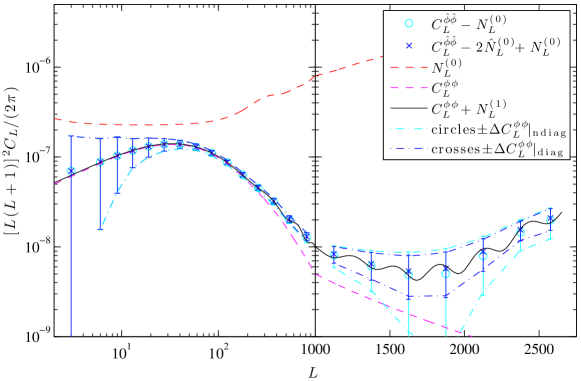
Figure 1: Reconstructed lensing potential power spectrum $C_{L}^{\hat{\phi}\hat{\phi}}$ averaged over $1000$ simulations, after subtracting the analytically-calculated $N^{(0)}$ bias (cyan circles). The magenta line is the input lensing potential power. Blue symbols include the empirical reconstruction bias correction of Eq. (17). The error bars show the estimated standard deviation of the binned power spectrum for a single realisation of the lensed CMB. Cyan error bars are only visible when they disagree from the blue error bars. Cyan dash-dotted lines show theoretical error bars obtained by binning Eqs. (28) and (29) below. Blue dash-dotted lines are theoretical error bars from Eq. (29) only. The biases $N^{(0)}$ (red) and $N^{(1)}$ (black, which also includes $C_{L}^{\phi\phi}$) are calculated analytically. Note that the left-hand panel uses a log scale for multipole $L$, whereas the right-hand panel uses a linear scale.

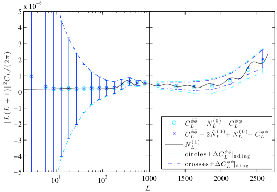
Figure 2: Same as Fig. 1 after subtracting the theoretical lensing power spectrum $C_{L}^{\phi\phi}$.

IV Auto-correlations of power spectra

We will argue later that parameter estimation with the lensing reconstruction should be based on empirical power spectra defined by

$$\hat{C}_{l}^{XX}\equiv\frac{1}{2l+1}\sum_{m=-l}^{l}(-1)^{m}\hat{X}_{lm}\hat{X}_{l,-m},$$ (19)

where $\hat{X}_{lm}$ are the multipole coefficients of the realisation $\hat{X}(\hat{\mathbf{n}})$ of a field on the sphere. Here, $X=\tilde{T}$ or $\phi$. To construct a likelihood for the empirical power spectra we will model auto- and cross-correlations of the empirical power spectra of the observed lensed temperature and the reconstructed lensing potential. If $X$ is a statistically-isotropic, Gaussian field, then the power covariance is diagonal with

$$\mathrm{cov}(\hat{C}^{XX}_{l},\hat{C}^{XX}_{l^{\prime}})=\delta_{ll^{\prime}}\frac{2}{2l+1}\langle\hat{C}_{l}^{XX}\rangle^{2}.$$ (20)

In the following we will abbreviate the Gaussian variance with

$$\mathrm{var}_{G}(C^{XX}_{l})\equiv\frac{2}{2l+1}\left(C^{XX}_{l}\right)^{2}.$$ (21)

We demonstrate in Appendix F that for most applications we can neglect the effect of $C^{T\phi}$ on the covariance between the power spectra of the lensed temperature and the lens reconstruction. Because the Taylor expansion of Eq. (2) is linear in the unlensed temperature all odd $n$-point functions of the lensed temperature vanish.

IV.1 Lensed temperature

The auto-correlation of the lensed temperature power spectrum has been computed at first order in $C^{\phi\phi}$ in Smith et al. (2006b) under the flat-sky approximation and in Li et al. (2007) on the full sky. A contribution at second order in $C^{\phi\phi}$ was recently identified in Benoit-Lévy et al. (2012). The power covariance is given by

$$\mathrm{cov}(\hat{C}^{\tilde{T}\tilde{T}}_{l,\mathrm{expt}},\hat{C}^{\tilde{T}\tilde{T}}_{l^{\prime},\mathrm{expt}})=\delta_{ll^{\prime}}\mathrm{var}_{G}(C^{\tilde{T}\tilde{T}}_{l,\mathrm{expt}})+\frac{1}{(2l+1)(2l^{\prime}+1)}\sum_{m,m^{\prime}}(-1)^{m+m^{\prime}}\langle\tilde{T}_{lm}\tilde{T}_{l,-m}\tilde{T}_{l^{\prime}m^{\prime}}\tilde{T}_{l^{\prime},-m^{\prime}}\rangle_{c},$$ (22)

where $\langle\,\rangle_{c}$ denotes the connected part of the $4$-point function, which is at $\mathcal{O}(C^{\phi\phi})$ Hu (2001b)

$$\langle\tilde{T}_{\underline{l}_{1}}\tilde{T}_{\underline{l}_{2}}\tilde{T}_{\underline{l}_{3}}\tilde{T}_{\underline{l}_{4}}\rangle_{c}=\frac{1}{2}C^{TT}_{l_{2}}C^{TT}_{l_{4}}\sum_{LM}(-1)^{M}C_{L}^{\phi\phi}\left(\begin{matrix}l_{1}&l_{2}&L\\ m_{1}&m_{2}&-M\end{matrix}\right)\left(\begin{matrix}l_{3}&l_{4}&L\\ m_{3}&m_{4}&M\end{matrix}\right)F_{l_{1}Ll_{2}}F_{l_{3}Ll_{4}}+\mbox{all perms.}$$ (23)

Here and in the following ‘all perms’ denotes permutations in all non-contracted multipole indices, i.e. permutations of $1$, $2$, $3$, and $4$ in Eq. (23). If we also include the contribution at second order in $C^{\phi\phi}$ from Benoit-Lévy et al. (2012) we get Li et al. (2007); Benoit-Lévy et al. (2012)

$$\mathrm{cov}(\hat{C}^{\tilde{T}\tilde{T}}_{l,\mathrm{expt}},\hat{C}^{\tilde{T}\tilde{T}}_{l^{\prime},\mathrm{expt}}) = \delta_{ll^{\prime}}\mathrm{var}_{G}(C^{\tilde{T}\tilde{T}}_{l,\mathrm{expt}})+\frac{2}{(2l+1)(2l^{\prime}+1)}\sum_{L}C^{\phi\phi}_{L}f^{2}_{lLl^{\prime}}$$ (24)

$$\;\;+\sum_{L}\frac{\partial C^{\tilde{T}\tilde{T}}_{l}}{\partial C^{\phi\phi}_{L}}\frac{2}{2L+1}\left(C^{\phi\phi}_{L}\right)^{2}\frac{\partial C^{\tilde{T}\tilde{T}}_{l^{\prime}}}{\partial C^{\phi\phi}_{L}}+\mathcal{O}[(C^{\phi\phi})^{3}],$$

where $f_{l_{1}Ll_{2}}$ is from the unlensed version of Eq. (8): $f_{l_{1}Ll_{2}}=C^{TT}_{l_{2}}F_{l_{1}Ll_{2}}+C^{TT}_{l_{1}}F_{l_{2}Ll_{1}}$. The third term on the right of Eq. (24) arises from cosmic variance of the lenses. Fluctuations at lens multipole $L$ produce fluctuations in the empirical lensed temperature power spectrum over a range of multipoles. The fluctuations in the lens power, $\Delta C_{L}^{\phi\phi}$, propagate to the empirical temperature power spectrum approximately as $\partial C^{\tilde{T}\tilde{T}}_{l}/\partial C_{L}^{\phi\phi}$. The power derivative here can be calculated perturbatively by noting that at $\mathcal{O}(C^{\phi\phi})$ Hu (2000)

$$C^{\tilde{T}\tilde{T}}_{l}=C_{l}^{TT}[1-l(l+1)R]+\sum\limits_{l_{1},l_{2}}C_{l_{1}}^{\phi\phi}C_{l_{2}}^{TT}\frac{F^{2}_{ll_{1}l_{2}}}{2l+1},$$ (25)

where

$$R=\frac{1}{8\pi}\sum\limits_{l}(2l+1)l(l+1)C_{l}^{\phi\phi}$$ (26)

is half the mean-squared deflection. Therefore

$$\frac{\partial C^{\tilde{T}\tilde{T}}_{l}}{\partial C^{\phi\phi}_{L}}=\sum_{l^{\prime}}C_{l^{\prime}}^{TT}\,\frac{F_{lLl^{\prime}}^{2}}{2l+1}-\frac{L(L+1)(2L+1)}{8\pi}\,l(l+1)C_{l}^{TT}.$$ (27)

While Ref. Benoit-Lévy et al. (2012) included higher-order corrections to this expression by taking numerical derivatives of lensed power spectra computed non-perturbatively with the CAMB code Lewis et al. (2000); Challinor and Lewis (2005), these corrections are not expected to be important for our purposes here.

The off-diagonal contributions to the correlation between the empirical $\hat{C}^{\tilde{T}\tilde{T}}_{l,\mathrm{expt}}$ are shown in Fig. 3 (see Li et al. (2007) and Benoit-Lévy et al. (2012) for similar plots). The checkerboard structure of the $\mathcal{O}[(C^{\phi\phi})^{2}]$ contribution arises because fluctuations in the lensing power produce changes in the lensed temperature spectra of opposite signs at the acoustic peaks and troughs. Both of the corrections in Eq. (24) give correlations that are at most of order $10^{-4}$ and are rather localised in the $(l,l^{\prime})$ plane. (Note that the correlations are suppressed on small scales where noise dominates the diagonal variance.) The impact of these non-diagonal contributions is found to be negligible for all calculations in this paper, i.e. we can assume a Gaussian diagonal auto-covariance of the temperature power spectrum.

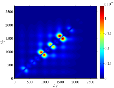
(a)

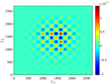
(b)

Figure 3: (a) Theoretical off-diagonal part of the correlation $\mathrm{correl}(\hat{C}^{\tilde{T}\tilde{T}}_{L_{T}},\hat{C}^{\tilde{T}\tilde{T}}_{L^{\prime}_{T}})$ to first order in $C^{\phi\phi}$, given by the second term on the right of Eq. (24) (see Li et al. (2007)). The covariance is converted to a correlation by dividing by $[\mathrm{var}_{G}(C^{\tilde{T}\tilde{T}}_{L_{T},\mathrm{expt}})\mathrm{var}_{G}(C^{\tilde{T}\tilde{T}}_{L^{\prime}_{T},\mathrm{expt}})]^{1/2}$. (b) $\mathcal{O}\left[(C^{\phi\phi})^{2}\right]$ contribution to the correlation identified in Benoit-Lévy et al. (2012).

IV.2 Lensing reconstruction

The auto-correlation of the lensing reconstruction power spectrum involves the $8$-point function of the lensed temperature. Hanson et al. Hanson et al. (2011) found that the dominant off-diagonal contributions on the full sky are given by disconnected terms that contribute as (see Kesden et al. (2003) for a similar calculation on the flat sky)

$$\mathrm{cov}(\hat{C}_{L}^{\hat{\phi}\hat{\phi}},\hat{C}_{L^{\prime}}^{\hat{\phi}\hat{\phi}})_{\text{non-diag}}^{\mathrm{dom}} = \frac{32A_{L}^{2}A_{L^{\prime}}^{2}}{(2L+1)(2L^{\prime}+1)}\sum_{l_{1}}\frac{1}{2l_{1}+1}(C^{\tilde{T}\tilde{T}}_{l_{1},\mathrm{expt}})^{2}\left[\sum_{l_{2}}\tilde{g}_{l_{1}l_{2}}^{2}(L)C^{\tilde{T}\tilde{T}}_{l_{2},\mathrm{expt}}\right]\left[\sum_{l_{3}}\tilde{g}_{l_{1}l_{3}}^{2}(L^{\prime})C^{\tilde{T}\tilde{T}}_{l_{3},\mathrm{expt}}\right].\;\;\;$$ (28)

This dominates over more tightly-coupled terms that involve products of four weights $\tilde{g}$ that do not factor in the form $\tilde{g}^{2}\tilde{g}^{2}$ and therefore enforce a reduced summation volume. The variance ($L=L^{\prime}$) on the full sky is predominantly

$$\mathrm{var}(\hat{C}_{L}^{\hat{\phi}\hat{\phi}})=\frac{2}{2L+1}\langle C_{L}^{\hat{\phi}\hat{\phi}}\rangle^{2},$$ (29)

with small corrections from Eq. (28) (for $L=L^{\prime}$).

As shown in Hanson et al. (2011) the off-diagonal reconstruction power correlation can reach a level of $0.5\%$ and is rather broad-band. If the reconstructed power is binned this can induce correlations of $\mathcal{O}(10\%)$ between different bins. Physically, these broad-band correlations arise because cosmic-variance fluctuations in the CMB at a given scale produce fluctuations in $\hat{C}^{\hat{\phi}\hat{\phi}}$ that are coherent over a broad range of scales due to the mode-coupling nature of lens reconstruction (small-scale CMB fluctuations are used to reconstruct large-scale lenses). To make this physical interpretation more explicit we note that the dominant non-diagonal covariance contribution of Eq. (28) can be written as

$$\mathrm{cov}(\hat{C}_{L}^{\hat{\phi}\hat{\phi}},\hat{C}_{L^{\prime}}^{\hat{\phi}\hat{\phi}})_{\text{non-diag}}^{\mathrm{dom}}=\sum_{l_{1}}\frac{\partial(2\hat{N}^{(0)}_{L})}{\partial\hat{C}^{\tilde{T}\tilde{T}}_{l_{1},\mathrm{expt}}}\;\frac{2}{2l_{1}+1}(C^{\tilde{T}\tilde{T}}_{l_{1},\mathrm{expt}})^{2}\;\frac{\partial(2\hat{N}^{(0)}_{L^{\prime}})}{\partial\hat{C}^{\tilde{T}\tilde{T}}_{l_{1},\mathrm{expt}}},$$ (30)

where the (realisation-independent) derivative is given by

$$\frac{\partial(2\hat{N}^{(0)}_{L})}{\partial\hat{C}^{\tilde{T}\tilde{T}}_{l_{1},\mathrm{expt}}}=\frac{4A_{L}^{2}}{2L+1}\sum\limits_{l_{2}}\tilde{g}^{2}_{l_{1}l_{2}}(L)C^{\tilde{T}\tilde{T}}_{l_{2},\mathrm{expt}},$$ (31)

which is non-zero even in the absence of lensing. Equation (31) describes the change of the Gaussian reconstruction noise resulting from fluctuations of the observed temperature realisation. In propagating these changes through to the covariance of $\hat{C}^{\hat{\phi}\hat{\phi}}$, one picks up the sample variance of the total lensed temperature power spectrum, $\mathrm{var}_{G}(C^{\tilde{T}\tilde{T}}_{l,\mathrm{expt}})$.

As noted in Sec. II, using the realisation-dependent $\hat{N}^{(0)}$ bias correction of Eq. (17) significantly reduces the off-diagonal covariance of the reconstruction power spectrum. To help interpret the $\hat{N}^{(0)}$ correction, we write it in the form

$$\hat{C}_{L}^{\hat{\phi}\hat{\phi}}-2\hat{N}_{L}^{(0)}+N_{L}^{(0)}=\hat{C}_{L}^{\hat{\phi}\hat{\phi}}-\sum_{l}\frac{\partial(2\hat{N}^{(0)}_{L})}{\partial\hat{C}^{\tilde{T}\tilde{T}}_{l,\mathrm{expt}}}\hat{C}^{\tilde{T}\tilde{T}}_{l,\mathrm{expt}}+N_{L}^{(0)}.$$ (32)

Therefore, for a given realisation of the lensed temperature, the empirical $\hat{N}^{(0)}$ bias correction partly removes the response of the Gaussian reconstruction noise to changes in the lensed temperature realisation. To see that this removes the non-diagonal power covariance of the lensing reconstruction caused by cosmic variance of the lensed temperature, note that both $\mathrm{cov}(\hat{C}^{\hat{\phi}\hat{\phi}}_{L},2\hat{N}^{(0)}_{L^{\prime}})$ and $\mathrm{cov}(2\hat{N}^{(0)}_{L},2\hat{N}^{(0)}_{L^{\prime}})$ equal the right hand side of Eq. (30) at $\mathcal{O}(\phi^{0})$. The empirical $\hat{N}^{(0)}$ correction leads to a small reduction in the variance of the binned reconstructed power spectrum, as shown in Figs. 1 and 2. Any residual covariance after empirical $\hat{N}^{(0)}$ subtraction is too small to be detected in our simulations.

V Temperature-lensing cross-correlation

For a joint analysis involving the empirical power spectra of the lens reconstruction and the lensed temperature anisotropies, the likelihood should model their cross-correlation to avoid potential double-counting of lensing effects. In this section we calculate the cross-correlation. We recover the two main physical effects introduced in Sec. I, i.e. a “noise contribution” from the cosmic variance of the lensed temperature affecting the noise in the reconstruction over a wide range of scales, and a “matter cosmic variance” contribution from cosmic variance of the lenses altering the smoothing of the acoustic peaks in the temperature power spectrum. We will show in Sec. V.1 that the noise contribution is due to the disconnected part of the lensed temperature $6$-point function, while in Sec. V.2 we show that the matter cosmic variance contribution is due to the connected part of the $6$-point function. Corrections from the lensed temperature trispectrum generally have a sub-dominant effect on parameter estimation and are discussed in Appendix D (see also Fig. 8 below).

V.1 Noise contribution

V.1.1 Perturbative derivation: Disconnected part of lensed temperature 4- and 6-point functions

Since the reconstructed lensing potential is quadratic in the lensed temperature the covariance $\mathrm{cov}(\hat{C}_{L}^{\hat{\phi}\hat{\phi}},\hat{C}_{L^{\prime},\mathrm{expt}}^{\tilde{T}\tilde{T}})$ involves the $4$- and $6$-point functions of the lensed temperature. Using the definition of $\hat{\phi}$ in (9) we find

$$\mathrm{cov}(\hat{C}_{L}^{\hat{\phi}\hat{\phi}},\hat{C}_{L^{\prime},\mathrm{expt}}^{\tilde{T}\tilde{T}}) = \frac{A_{L}^{2}}{(2L+1)(2L^{\prime}+1)}\sum\limits_{\underline{l}_{1},\underline{l}_{2},\underline{l}_{3},\underline{l}_{4},M,M^{\prime}}(-1)^{M+M^{\prime}}\left(\begin{matrix}l_{1}&l_{2}&L\\ m_{1}&m_{2}&-M\end{matrix}\right)\left(\begin{matrix}l_{3}&l_{4}&L\\ m_{3}&m_{4}&M\end{matrix}\right)\tilde{g}_{l_{1}l_{2}}(L)\tilde{g}_{l_{3}l_{4}}(L)$$ (33)

$$\;\times\left[\langle\tilde{T}_{\underline{l}_{1}}\tilde{T}_{\underline{l}_{2}}\tilde{T}_{\underline{l}_{3}}\tilde{T}_{\underline{l}_{4}}\tilde{T}_{L^{\prime}M^{\prime}}\tilde{T}_{L^{\prime},-M^{\prime}}\rangle-\langle\tilde{T}_{\underline{l}_{1}}\tilde{T}_{\underline{l}_{2}}\tilde{T}_{\underline{l}_{3}}\tilde{T}_{\underline{l}_{4}}\rangle\langle\tilde{T}_{L^{\prime}M^{\prime}}\tilde{T}_{L^{\prime},-M^{\prime}}\rangle\right].$$

Since all connected terms vanish in the absence of lensing we expect the noise contribution to come from the fully disconnected part. If we only keep disconnected terms, the second line of Eq. (33) can be replaced by

$$\left[\langle\tilde{T}_{\underline{l}_{1}}\tilde{T}_{\underline{l}_{2}}\tilde{T}_{\underline{l}_{3}}\tilde{T}_{\underline{l}_{4}}\tilde{T}_{L^{\prime}M^{\prime}}\tilde{T}_{L^{\prime},-M^{\prime}}\rangle-\langle\tilde{T}_{\underline{l}_{1}}\tilde{T}_{\underline{l}_{2}}\tilde{T}_{\underline{l}_{3}}\tilde{T}_{\underline{l}_{4}}\rangle\langle\tilde{T}_{L^{\prime}M^{\prime}}\tilde{T}_{L^{\prime},-M^{\prime}}\rangle\right]\rightarrow 4\left[\langle\tilde{T}_{\underline{l}_{1}}\tilde{T}_{\underline{l}_{3}}\rangle\langle\tilde{T}_{\underline{l}_{2}}\tilde{T}_{L^{\prime}M^{\prime}}\rangle\langle\tilde{T}_{\underline{l}_{4}}\tilde{T}_{L^{\prime},-M^{\prime}}\rangle+(M^{\prime}\leftrightarrow-M^{\prime})\right],$$ (34)

where we exploited symmetry under relabeling $(\underline{l}_{1}\leftrightarrow\underline{l}_{2})$ and/or $(\underline{l}_{3}\leftrightarrow\underline{l}_{4})$. We also used that the contractions $\langle\tilde{T}_{\underline{l}_{1}}\tilde{T}_{\underline{l}_{2}}\rangle$ and $\langle\tilde{T}_{\underline{l}_{3}}\tilde{T}_{\underline{l}_{4}}\rangle$ do not contribute because $\langle\hat{\phi}_{LM}\rangle=0$. The fully disconnected part of Eq. (33) is therefore

$$\mathrm{cov}(\hat{C}_{L}^{\hat{\phi}\hat{\phi}},\hat{C}_{L^{\prime},\mathrm{expt}}^{\tilde{T}\tilde{T}})_{\mathrm{disconn.}}=\frac{8A_{L}^{2}}{(2L+1)(2L^{\prime}+1)}\left(C_{L^{\prime},\mathrm{expt}}^{\tilde{T}\tilde{T}}\right)^{2}\sum\limits_{l_{1}}\tilde{g}^{2}_{l_{1}L^{\prime}}(L)C_{l_{1},\mathrm{expt}}^{\tilde{T}\tilde{T}},$$ (35)

where the weight $\tilde{g}_{l_{1}L^{\prime}}(L)$ enforces $l_{1}+L+L^{\prime}$ to be even.

To interpret this result note that it can be expressed in terms of the derivative in Eq. (31) as

$$\mathrm{cov}(\hat{C}^{\hat{\phi}\hat{\phi}}_{L},\hat{C}^{\tilde{T}\tilde{T}}_{L^{\prime},\mathrm{expt}})_{\mathrm{disconn.}}=\frac{\partial(2\hat{N}^{(0)}_{L})}{\partial\hat{C}^{\tilde{T}\tilde{T}}_{L^{\prime},\mathrm{expt}}}\,\frac{2}{2L^{\prime}+1}\left(C^{\tilde{T}\tilde{T}}_{L^{\prime},\mathrm{expt}}\right)^{2}.$$ (36)

This part of the covariance is therefore due to the response of the Gaussian reconstruction noise to changes in the observed temperature realisation and the resulting covariance with the observed temperature power. Based on this intuition, we anticipate that the covariance can be mitigated by the realisation-dependent $\hat{N}^{(0)}$ correction of the reconstruction power bias (see Sec. V.1.4 for confirmation).

V.1.2 Magnitude and structure of the correlation matrix

In Fig. 4a we plot the power correlation resulting from the power covariance in Eq. (35) (denoting $L_{\phi}=L$ and $L_{T}=L^{\prime}$ for convenience),

$$\mathrm{correl}(\hat{C}^{\hat{\phi}\hat{\phi}}_{L_{\phi}},\hat{C}^{\tilde{T}\tilde{T}}_{L_{T},\mathrm{expt}})=\frac{\mathrm{cov}(\hat{C}^{\hat{\phi}\hat{\phi}}_{L_{\phi}},\hat{C}^{\tilde{T}\tilde{T}}_{L_{T},\mathrm{expt}})}{\sqrt{\mathrm{var}_{G}(C^{\phi\phi}_{L_{\phi}}+N^{(0)}_{L_{\phi}}+N^{(1)}_{L_{\phi}})\,\mathrm{var}_{G}(C^{\tilde{T}\tilde{T}}_{L_{T},\mathrm{expt}})}}.$$ (37)

We plot the correlation of the unbinned spectra. Note that if the covariance is broad-band (i.e. roughly constant over the bin width) the correlation of (sufficiently finely) binned power spectra will increase roughly proportionally to the square root of the product of the two bin widths. The Gaussian variance of $C^{\tilde{T}\tilde{T}}_{L_{T},\mathrm{expt}}$ in the denominator of Eq. (37) contains the beam-deconvolved noisy temperature power spectrum (18), so that high temperature multipoles are suppressed.

(a)

(b)

(c)

Figure 4: (a) Theoretical noise contribution from Eq. (35) to the correlation of unbinned power spectra of the lensed temperature and the reconstructed lensing potential, $\mathrm{correl}(\hat{C}_{L_{\phi}}^{\hat{\phi}\hat{\phi}},\hat{C}_{L_{T},\mathrm{expt}}^{\tilde{T}\tilde{T}})$. The acoustic peaks of the temperature power spectrum are visible in the vertical direction. (b) Estimate of the correlation of unbinned power spectra from $1000$ simulations. (c) Same as (b) after subtracting the empirical $\hat{N}^{(0)}$ bias of Eq. (17) from $\hat{C}^{\hat{\phi}\hat{\phi}}$.

The unbinned power correlation shown in Fig. 4a is mostly constrained to a cone-like region in the $L_{\phi}$ vs $L_{T}$ plane, with the maximum correlation of $0.5\%$ located at the first acoustic peak $L_{T}\sim 200$ and lensing reconstruction multipoles $1600\lesssim L_{\phi}\lesssim 1900$. To understand the basic structure of the correlation in Fig. 4a we compute approximations to Eq. (35) in the limits $L_{T}\ll L_{\phi}$ and $L_{\phi}\ll L_{T}$.

For $L_{T}\ll L_{\phi}$, the weights in Eq. (35) restrict the summation from $l_{1}=L_{\phi}-L_{T}$ to $l_{1}=L_{\phi}+L_{T}$. If we Taylor expand in $l_{1}$ around $L_{\phi}$ we get

$$\mathrm{correl}(\hat{C}^{\hat{\phi}\hat{\phi}}_{L_{\phi}},\hat{C}^{\tilde{T}\tilde{T}}_{L_{T},\mathrm{expt}})_{\mathrm{disconn.}}^{L_{T}\ll L_{\phi}}\approx\frac{[L_{\phi}(L_{\phi}+1)]^{2}A_{L_{\phi}}}{8\pi}\sqrt{(2L_{T}+1)(2L_{\phi}+1)}\;\frac{L_{T}(L_{T}+1)C^{\tilde{T}\tilde{T}}_{L_{T}}}{L_{\phi}(L_{\phi}+1)C^{\tilde{T}\tilde{T}}_{L_{\phi},\mathrm{expt}}}.$$ (38)

Recalling that $A_{L_{\phi}}=N_{L_{\phi}}^{(0)}$ for optimal weights, we see from Fig. 1 that the first term slightly increases with $L_{\phi}$. The last term is maximised at the first acoustic peak $L_{T}\sim 200$ and at the reconstruction multipole $1600\lesssim L_{\phi}\lesssim 1900$ where the observed temperature power $C^{\tilde{T}\tilde{T}}_{L_{\phi},\mathrm{expt}}$ is minimal (for the Planck-like noise and beam considered here). In this region Eq. (38) gives a correlation of around $0.4$–$0.5\%$, which agrees with Fig. 4a. Equation (38) also implies that lower noise in the temperature power spectrum would move the peak position to higher reconstruction multipoles $L_{\phi}$. The cone structure in Fig. 4a, with apex at $(L_{\phi},L_{T})\sim(\text{1600--1900},200)$ and edges $L_{\phi}-L_{T}\lesssim(\text{1600--1900})\lesssim L_{\phi}+L_{T}$, encloses the region for which the sum over $l_{1}$ includes the maximum of $1/C_{l_{1},\text{expt}}^{\tilde{T}\tilde{T}}$ around $l_{1}=1600$–$1900$. A similar argument can be applied for the cone patterns in the $L_{\phi}\lesssim 200$ region.

For high temperature and low reconstruction multipoles, $L_{\phi}\ll L_{T}$, we can Taylor expand Eq. (35) in $l_{1}$ around $L_{T}$ (see Hanson et al. (2011) for a similar calculation):

$$\mathrm{correl}(\hat{C}^{\hat{\phi}\hat{\phi}}_{L_{\phi}},\hat{C}^{\tilde{T}\tilde{T}}_{L_{T},\mathrm{expt}})_{\mathrm{disconn.}}^{L_{\phi}\ll L_{T}} \approx \frac{[L_{\phi}(L_{\phi}+1)]^{2}A_{L_{\phi}}^{2}}{2\pi(A_{L_{\phi}}+C^{\phi\phi}_{L_{\phi}})}\left(\frac{C^{\tilde{T}\tilde{T}}_{L_{T}}}{C^{\tilde{T}\tilde{T}}_{L_{T},\mathrm{expt}}}\right)^{2}\sqrt{\frac{(2{L_{\phi}}+1)(2L_{T}+1)}{4}}$$ (39)

$$\quad\times\;\frac{1}{4}\left[\left(\frac{\mathrm{d}\ln(L_{T}^{2}C^{\tilde{T}\tilde{T}}_{L_{T}})}{\mathrm{d}\ln L_{T}}\right)^{2}+\frac{1}{2}\,\left(\frac{\mathrm{d}\ln C^{\tilde{T}\tilde{T}}_{L_{T}}}{\mathrm{d}\ln L_{T}}\right)^{2}\right],$$

where we have neglected $N_{L_{\phi}}^{(1)}$ and used $A_{L_{\phi}}=N_{L_{\phi}}^{(0)}$. The quadrature sum of derivatives in the last term is maximal between acoustic peaks and troughs at $L_{T}\sim 350$, $625$, $925$, $1225$, $1550$, $1850$ etc., which agrees with the temperature multipoles where the full correlation shown in Fig. 4a is maximal (for $L_{\phi}\lesssim 200)$. The maximum value of the second line of Eq. (39) is around $36$ (for $L_{T}\lesssim 2700$). If we neglect $C^{\phi\phi}_{L_{\phi}}$ compared to $A_{L_{\phi}}$, which is roughly acceptable for $L_{\phi}\lesssim 10$, then the first term in Eq. (39) is around $2\times 10^{-7}$ (see Fig. 1), i.e. for ${L_{\phi}}\lesssim 10$,

$$\mathrm{correl}(\hat{C}^{\hat{\phi}\hat{\phi}}_{L_{\phi}},\hat{C}^{\tilde{T}\tilde{T}}_{L_{T},\mathrm{expt}})_{\mathrm{disconn.}}^{{L_{\phi}}\ll L_{T}}\lesssim 2\times 10^{-7}\times\frac{1}{2}\sqrt{(2{L_{\phi}}+1)(2L_{T}+1)}\times 36.$$ (40)

For example, for ${L_{\phi}}=10$, $L_{T}=1500$ the bound is $9\times 10^{-4}$ which is consistent with the full result shown in Fig. 4a.

V.1.3 Comparison with simulations

Before assessing the relevance of the noise contribution to the covariance for parameter estimation we compare the analytic result in Eq. (35) with the full covariance estimated from our simulations. For the latter, we use

$$\widehat{\mathrm{cov}}(\hat{C}^{\hat{\phi}\hat{\phi}}_{{L}},\hat{C}^{\tilde{T}\tilde{T}}_{{L^{\prime}},\mathrm{expt}})=\frac{1}{N_{\mathrm{sims}}-1}\sum_{s=1}^{N_{\mathrm{sims}}}(\hat{C}^{\hat{\phi}\hat{\phi}}_{L,s}-\langle\hat{C}^{\hat{\phi}\hat{\phi}}_{L}\rangle_{\mathrm{sims}})(\hat{C}^{\tilde{T}\tilde{T}}_{L^{\prime},\mathrm{expt},s}-\langle\hat{C}^{\tilde{T}\tilde{T}}_{L^{\prime},\mathrm{expt}}\rangle_{\mathrm{sims}}),$$ (41)

where $s$ labels different realisations and $\langle\cdot\rangle_{\mathrm{sims}}$ denotes the average over $N_{\mathrm{sims}}$ realisations. To reduce the noise of the estimates from the finite number of simulations, we average the measured covariance over a range of $L$ and $L^{\prime}$ values,

$$\widehat{\mathrm{cov}}(\hat{C}^{\hat{\phi}\hat{\phi}}_{\overline{L}_{i}},\hat{C}^{\tilde{T}\tilde{T}}_{\overline{L}^{\prime}_{j},\mathrm{expt}})=\frac{1}{\Delta L_{i}\Delta L^{\prime}_{j}}\frac{1}{[\overline{L}_{i}(\overline{L}_{i}+1)]^{2}\;\overline{L}^{\prime}_{j}(\overline{L}^{\prime}_{j}+1)}\sum_{L=L_{i}}^{L_{i+1}-1}\sum_{L^{\prime}=L^{\prime}_{j}}^{L^{\prime}_{j+1}-1}[L(L+1)]^{2}L^{\prime}(L^{\prime}+1)\widehat{\mathrm{cov}}(\hat{C}^{\hat{\phi}\hat{\phi}}_{L},\hat{C}^{\tilde{T}\tilde{T}}_{L^{\prime}}),$$ (42)

where $L_{i}$ and $L^{\prime}_{j}$ are bin boundaries for lensing and temperature powers, respectively, and $\overline{L}_{i}$ and $\overline{L}^{\prime}_{j}$ denote the corresponding bin centres. The bin widths are $\Delta L_{i}=L_{i+1}-L_{i}$ and $\Delta L^{\prime}_{j}=L^{\prime}_{j+1}-L^{\prime}_{j}$. We divide out $L(L+1)$ prefactors to average over relatively slowly varying quantities. In Fig. 4b we plot the estimate of the correlation that unbinned power spectra would have. This is obtained by dividing the covariance estimate of Eq. (42) by the theoretical Gaussian variance of unbinned power spectra as in Eq. (37) [evaluated at $(\overline{L}_{i},\overline{L^{\prime}}_{j})$]. Within the random scatter from the finite $N_{\text{sims}}$, the estimated correlation agrees with the theoretical noise contribution of Eq. (35). We can also conclude that the noise contribution is the dominant part of the temperature-lensing power correlation.

V.1.4 Mitigating the noise contribution with the empirical $\hat{N}^{(0)}$ bias correction

In practice, it is desirable that the temperature and reconstruction power spectra are uncorrelated so that their respective likelihoods may be simply combined. Indeed, this is the assumption that has been made in all joint analyses to date Sherwin et al. (2011); van Engelen et al. (2012); Planck Collaboration et al. (2013a).

Fortunately, the empirical $\hat{N}^{(0)}$ subtraction, which was originally proposed in Hanson et al. (2011) to eliminate the non-diagonal reconstruction power auto-covariance (28), also removes the noise contribution [Eq. (35)] to the temperature-lensing power cross-covariance. To see this note that if the empirical bias correction of Eq. (17) is used, the cross-covariance changes by

$$-\mathrm{cov}(2\hat{N}^{(0)}_{L},\hat{C}_{L^{\prime},\mathrm{expt}}^{\tilde{T}\tilde{T}})=-\sum_{l}\frac{\partial(2\hat{N}^{(0)}_{L})}{\partial\hat{C}^{\tilde{T}\tilde{T}}_{l,\mathrm{expt}}}\mathrm{cov}(\hat{C}^{\tilde{T}\tilde{T}}_{l,\mathrm{expt}},\hat{C}^{\tilde{T}\tilde{T}}_{L^{\prime},\mathrm{expt}})=-\mathrm{cov}(\hat{C}^{\hat{\phi}\hat{\phi}}_{L},\hat{C}_{L^{\prime},\mathrm{expt}}^{\tilde{T}\tilde{T}})_{\mathrm{disconn.}}+\mathcal{O}(\phi^{2}).$$ (43)

We establish a more general version of this result in Appendix B, where we show that the generalisation of the $\hat{N}^{(0)}$ correction for anisotropic surveys removes the noise contribution to the covariance with any quadratic estimate (including e.g. cross-spectra) of the temperature power spectrum. We confirm the reduction in the cross-covariance with simulations in Fig. 4c. Corrections to Eq. (43) from the non-Gaussian terms in the covariance of the temperature power spectra [see Eq. (24)] at $\mathcal{O}(\phi^{2})$ and $\mathcal{O}(\phi^{4})$ reach at most $3\times 10^{-5}$ in the correlation, which is roughly one order of magnitude smaller than the matter cosmic variance contribution discussed below (see Fig. 5a). These corrections are too small to be visible in Fig. 4c and we neglect them in the following.

V.2 Matter cosmic variance contribution

V.2.1 Warm-up: Power covariance of input lensing potential and lensed temperature

We expect the cosmic variance of the lenses to induce a power-correlation of the lensed temperature with the lensing reconstruction since greater lensing power in a given realisation leads to additional smoothing of the empirical temperature power spectrum. As a warm-up, we calculate how the same effect gives rise to a covariance between the power spectrum of the temperature and the (unobservable) power spectrum of the lensing potential, as if we were able to measure $\phi$ directly with no noise. This correlation can be extracted from simulations simply by measuring the correlation of the power spectra of the lensed temperature and the input lensing potential without performing any lensing reconstruction. To calculate the covariance perturbatively, note that for a fixed realisation of the input lensing potential $\phi_{\mathrm{in}}$ the lensed temperature power spectrum obtained by averaging only over the unlensed CMB is given by ($L^{\prime}\neq 0$)

$$\frac{1}{2L^{\prime}+1}\sum_{M^{\prime}}\langle|\tilde{T}_{L^{\prime}M^{\prime}}|^{2}\rangle_{\mathrm{CMB}} = C_{L^{\prime}}^{TT}+\frac{1}{2L^{\prime}+1}\sum_{l_{1}l_{2}}\hat{C}_{l_{1}}^{\phi_{\mathrm{in}}\phi_{\mathrm{in}}}C_{l_{2}}^{TT}F_{L^{\prime}l_{1}l_{2}}^{2}-\hat{R}L^{\prime}(L^{\prime}+1)C_{L^{\prime}}^{TT}$$ (44)

$$= C_{L^{\prime}}^{TT}+\sum_{L^{\prime\prime}}\frac{\partial C^{\tilde{T}\tilde{T}}_{L^{\prime}}}{\partial C^{\phi\phi}_{L^{\prime\prime}}}\hat{C}^{\phi_{\mathrm{in}}\phi_{\mathrm{in}}}_{L^{\prime\prime}}.$$

Here $\hat{C}^{\phi_{\mathrm{in}}\phi_{\mathrm{in}}}$ denotes the empirical power spectrum of the input lensing potential realisation $\phi_{\mathrm{in}}$ and $\hat{R}$ is defined by replacing $C^{\phi\phi}$ in Eq. (26) by $\hat{C}^{\phi_{\mathrm{in}}\phi_{\mathrm{in}}}$. The first line of Eq. (44) can be derived from the expansion in Eq. (2) at second order in $\phi_{\mathrm{in}}$. The term linear in $\phi_{\mathrm{in}}$ vanishes because it is proportional to the monopole of $\phi_{\text{in}}$. In Eq. (44) we neglected noise in the temperature measurement since this does not contribute to the covariance that we aim to calculate. The derivative in the second line of Eq. (44) is given by Eq. (27). Neglecting the $T$-$\phi$ correlation, we then have

$$\mathrm{cov}(\hat{C}^{\phi_{\mathrm{in}}\phi_{\mathrm{in}}}_{L},\hat{C}^{\tilde{T}\tilde{T}}_{L^{\prime},\mathrm{expt}}) =\langle\hat{C}^{\phi_{\mathrm{in}}\phi_{\mathrm{in}}}_{L}\langle\hat{C}^{\tilde{T}\tilde{T}}_{L^{\prime},\mathrm{expt}}\rangle_{\text{CMB}}\rangle_{\text{LSS}}-\langle\hat{C}^{\phi_{\mathrm{in}}\phi_{\mathrm{in}}}_{L}\rangle\langle\hat{C}^{\tilde{T}\tilde{T}}_{L^{\prime},\mathrm{expt}}\rangle,$$

$$=\frac{2}{2L+1}(C^{\phi\phi}_{L})^{2}\,\frac{\partial C^{\tilde{T}\tilde{T}}_{L^{\prime}}}{\partial C^{\phi\phi}_{L}},$$ (45)

where $\langle\cdot\rangle_{\text{LSS}}$ denotes an average over realisations of $\phi$ (i.e., over large-scale structure).

V.2.2 Power covariance of reconstructed lenses and lensed temperature from the connected 6-point function

The power covariance [Eq. (33)] of the reconstructed lensing potential and the lensed temperature receives contributions from the connected $4$- and $6$-point functions, as well as the Gaussian (disconnected) part. The leading-order trispectrum is linear in $C^{\phi\phi}$ and so cannot give rise to the expected matter cosmic variance contribution calculated above. The trispectrum contributions are discussed in detail in Appendix D, and are shown to have a sub-dominant effect on parameter estimation (see Fig. 8 below). We therefore focus here on the contribution from the connected $6$-point function. Terms independent of $\phi$ do not contribute to the connected part and terms linear in $\phi$ vanish when averaging over large-scale structure. Since the $\phi^{2}$ contribution can be shown to vanish Kesden et al. (2002) as well as $\phi^{3}$ terms which vanish for Gaussian $\phi$, the leading-order contribution is of order $\phi^{4}$. The $\mathcal{O}(\phi^{4})$ contribution from the connected $6$-point function to the temperature-lensing power covariance is calculated in detail in Appendix E. The dominant contribution there [Eq. (111)] is exactly of the form calculated above [Eq. (45)] for the power covariance of the input lensing potential and the lensed temperature.

V.2.3 Magnitude and structure of the covariance matrix

The correlation of unbinned temperature and lensing power spectra due to Eq. (111) is at most $0.04\%$ (see Fig. 5a). Since higher lensing power lowers the acoustic peaks and increases the troughs of the temperature power spectrum, the correlation is negative at multipoles $L_{T}$ where the temperature power peaks and positive where it has a trough. The correlation is small for $L_{\phi}\gtrsim 150$ because the acoustic peak smearing is mainly caused by large-scale lenses Smith et al. (2006b).

(a)

(b)

Figure 5: (a) Theoretical matter cosmic variance contribution, from Eq. (111), to the correlation of the unbinned power spectra of the reconstructed lensing potential and the lensed temperature anisotropies. The covariance is converted to a correlation following Eq. (37). (b) Measured correlation $\widehat{\mathrm{correl}}(\hat{C}_{L_{\phi}}^{\phi_{\mathrm{in}}\phi_{\mathrm{in}}},\hat{C}_{L_{T}}^{\tilde{T}\tilde{T}}-\hat{C}^{TT}_{L_{T}})$ of the power spectrum of the input lensing potential and the difference of noise-free lensed and unlensed temperature power spectra from $1000$ simulations.

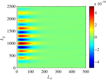
Figure 6: Left: The approximate contribution to the covariance between $[L_{\phi}(L_{\phi}+1)]^{2}\hat{C}_{L_{\phi}}^{\hat{\phi}\hat{\phi}}/(2\pi)$ and $L_{T}(L_{T}+1)\hat{C}_{L_{T}}^{\tilde{T}\tilde{T}}/(2\pi)$ from cosmic variance of the lenses, derived from Eq. (111). Right: The rank-one approximation to the matrix on the left from retaining only the largest singular value.

The approximate covariance matrix between $[L(L+1)]^{2}\hat{C}_{L}^{\hat{\phi}\hat{\phi}}/(2\pi)$ and $L^{\prime}(L^{\prime}+1)\hat{C}_{L^{\prime}}^{\tilde{T}\tilde{T}}/(2\pi)$, calculated from Eq. (111), is shown in the left-hand panel of Fig. 6. By perfoming a singular-value decomposition of this matrix, we find that it has a very low-rank structure. For example, retaining the multipoles of the reconstruction to $L=500$ (and up to $L^{\prime}=2500$ for the temperature), the first singular value is 34 times larger than the second. The covariance matrix can be accurately approximated in rank-one form,

$$\text{cov}\left(\frac{[L(L+1)]^{2}\hat{C}_{L}^{\hat{\phi}\hat{\phi}}}{2\pi},\frac{L^{\prime}(L^{\prime}+1)\hat{C}_{L^{\prime}}^{\tilde{T}\tilde{T}}}{2\pi}\right)_{\eqref{eq:matter_contri_theo}}\approx\lambda_{1}u_{L}v_{L^{\prime}},$$ (46)

as shown in the right-hand panel of Fig. 6. Here, the leading singular value $\lambda_{1}=8.3\times 10^{-8}\,\mu\mathrm{K}^{2}$; the corresponding (normalised) singular vectors $u_{L}$ (for the reconstructed lensing power) and $v_{L^{\prime}}$ (for the temperature power) are plotted in Fig. 7. The significance of the rank-one covariance is that cosmic variance of the lenses produces correlated changes in the measured lensed temperature power spectrum with definite shape given by $v_{L^{\prime}}$. Moreover, cosmic-variance fluctuations in $\hat{C}_{L}^{\phi\phi}$ that are orthogonal to $u_{L}$ do not influence $\hat{C}_{L^{\prime}}^{\tilde{T}\tilde{T}}$.

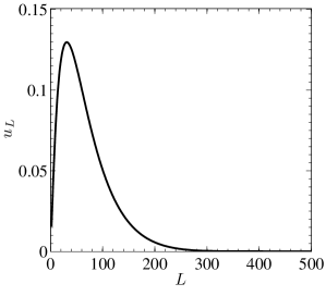
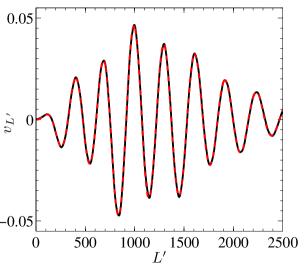
Figure 7: Singular vectors $u_{L}$ (left) and $v_{L^{\prime}}$ (right, black) of the matter cosmic variance contribution to the covariance between $[L(L+1)]^{2}\hat{C}_{L}^{\hat{\phi}\hat{\phi}}/(2\pi)$ and $L^{\prime}(L^{\prime}+1)\hat{C}_{L^{\prime}}^{\tilde{T}\tilde{T}}/(2\pi)$ corresponding to the dominant singular value; see Eq. (46). The approximation of Eq. (49) is shown in red dashed on the right.

We can understand the low-rank stucture of the covariance by evaluating the derivative $\partial C_{L^{\prime}}^{\tilde{T}\tilde{T}}/\partial C_{L}^{\phi\phi}$ with the flat-sky form of Eq. (25). Following Ref. Hu (2000), we have

$$C_{L^{\prime}}^{\tilde{T}\tilde{T}}=(1-{L^{\prime}}^{2}R)C_{L^{\prime}}^{TT}+\int\frac{d^{2}{\mathbf{L}}}{(2\pi)^{2}}\left[({\mathbf{L}}^{\prime}-{\mathbf{L}})\cdot{\mathbf{L}}\right]^{2}C_{L}^{\phi\phi}C^{TT}_{|{\mathbf{L}}^{\prime}-{\mathbf{L}}|},$$ (47)

where $R$ is given by Eq. (26). It is clear from Fig. 6 that the covariance is only significant between large-scale lens modes ($L<100$) and intermediate- and small-scale temperature modes (where lensing has a significant effect on the power spectrum). In the limit $L\ll L^{\prime}$, and for $L$ small compared to the CMB acoustic scale, we can Taylor expand $C^{TT}_{|{\mathbf{L}}^{\prime}-{\mathbf{L}}|}$ in Eq. (47) to obtain

$$\frac{\partial C_{L^{\prime}}^{\tilde{T}\tilde{T}}}{\partial C_{L}^{\phi\phi}}\approx\frac{L^{5}}{16{L^{\prime}}^{2}}\left[5L^{\prime}\frac{d}{dL^{\prime}}\left(\frac{L^{\prime}(L^{\prime}+1)C_{L^{\prime}}^{TT}}{2\pi}\right)+3{L^{\prime}}^{2}\frac{d^{2}}{d{L^{\prime}}^{2}}\left(\frac{L^{\prime}(L^{\prime}+1)C_{L^{\prime}}^{TT}}{2\pi}\right)\right]$$ (48)

at leading order in $L/L^{\prime}$. Since this is a rank-one matrix, the same is true of the covariance between $\hat{C}_{L}^{\hat{\phi}\hat{\phi}}$ and $\hat{C}_{L^{\prime}}^{\tilde{T}\tilde{T}}$. We can read off that the singular vector $v_{L^{\prime}}$ in Eq. (46) is

$$v_{L^{\prime}}\propto 5L^{\prime}\frac{d}{dL^{\prime}}\left(\frac{L^{\prime}(L^{\prime}+1)C_{L^{\prime}}^{TT}}{2\pi}\right)+3{L^{\prime}}^{2}\frac{d^{2}}{d{L^{\prime}}^{2}}\left(\frac{L^{\prime}(L^{\prime}+1)C_{L^{\prime}}^{TT}}{2\pi}\right),$$ (49)

which agrees well with that determined directly by singular-value decomposition (see Fig. 7). This singular vector is also similar to the change in $C_{L}^{TT}$ due to lensing over the acoustic part of the spectrum, where the dominant contribution is from large-scale lenses. Finally, we note that the rank-one structure of the derivative $\partial C_{L^{\prime}}^{\tilde{T}\tilde{T}}/\partial C_{L}^{\phi\phi}$ is consistent with the findings of Ref. Smith et al. (2006b) where it is shown that the lensed temperature power spectrum is sensitive to essentially a single mode of $C_{L}^{\phi\phi}$.

V.2.4 Comparison with simulations

Before assessing the importance for parameter estimation of the matter cosmic variance contribution to the cross-covariance, we validate it against simulations. The measurements of the temperature-lensing power correlation in Fig. 4b are too noisy to resolve clearly the matter cosmic variance contribution. However, we can test Eq. (45) by correlating the lensed temperature with the empirical power spectrum $\hat{C}^{\phi_{\mathrm{in}}\phi_{\mathrm{in}}}$ of the realisation of the input lensing potential without performing any reconstruction. To reduce the noise of the covariance estimate we work with the empirical power of the lensed temperature without including beam effects or noise, which do not affect the matter cosmic variance effect we are looking for. Since we have so far neglected $T$-$\phi$ correlations in all calculations, we try to eliminate correlations between the lensing potential and the unlensed temperature in the simulations by calculating $\widehat{\mathrm{cov}}(\hat{C}^{\phi_{\mathrm{in}}\phi_{\mathrm{in}}}_{L},\hat{C}^{\tilde{T}\tilde{T}}_{L^{\prime}}-\hat{C}^{TT}_{L^{\prime}})$. Here, $\hat{C}^{\phi_{\mathrm{in}}\phi_{\mathrm{in}}}$ is the empirical power of the input lensing potential and $\hat{C}^{TT}$ is the empirical power of the unlensed temperature. Additionally, subtracting the unlensed from the lensed empirical temperature power reduces the noise of the covariance estimate because it eliminates the scatter due to cosmic variance of the unlensed temperature. Otherwise, our estimate of the covariance follows the procedure described in Sec. V.1.3. As shown in Fig. 5b, these broad-band estimates are consistent with the theoretical expectation from Eq. (45).

V.2.5 Mitigating the matter cosmic variance contribution

As we shall show in Sec. V.4, the impact on parameter errors of ignoring the covariance between the lensed temperature and reconstruction power due to cosmic variance of the lenses is small for an experiment like Planck. Indeed, this is why the covariance is not accounted for in the current Planck likelihood Planck Collaboration et al. (2013a). However, the covariance is simple to model using Eq. (111) and could easily be included in a joint analysis. Equivalently, the covariance could be diagonalised by appropriate modifications of the empiricial temperature or lensing power spectra. A symmetric way to do this, mirroring the empirical $N^{(0)}$ correction that we advocate applying to the empirical lensing reconstruction power, is to modify the measured temperature power spectrum by

$$\hat{C}^{\tilde{T}\tilde{T}}_{l,\mathrm{expt}}\rightarrow\hat{C}^{\tilde{T}\tilde{T}}_{l,\mathrm{expt}}-\sum_{l^{\prime}}A_{ll^{\prime}}(\hat{C}_{l^{\prime}}^{\hat{\phi}\hat{\phi}}-2\hat{N}_{l^{\prime}}^{(0)})+\left\langle\sum_{l^{\prime}}A_{ll^{\prime}}(\hat{C}_{l^{\prime}}^{\hat{\phi}\hat{\phi}}-2\hat{N}_{l^{\prime}}^{(0)})\right\rangle,$$ (50)

where

$$A_{ll^{\prime}}=\frac{\partial C_{l}^{\tilde{T}\tilde{T}}}{\partial C_{l^{\prime}}^{\phi\phi}}\left(\frac{C_{l^{\prime}}^{\phi\phi}}{\langle\hat{C}_{l^{\prime}}^{\hat{\phi}\hat{\phi}}\rangle}\right)^{2}.$$ (51)

The expectation value is introduced in Eq. (50) to preserve the mean value of $\hat{C}^{\tilde{T}\tilde{T}}_{l,\mathrm{expt}}$. The construct $(C_{l^{\prime}}^{\phi\phi}/\langle\hat{C}_{l^{\prime}}^{\hat{\phi}\hat{\phi}}\rangle)^{2}$ acts like a Wiener filter on the empirical spectrum $\hat{C}_{l^{\prime}}^{\hat{\phi}\hat{\phi}}-2\hat{N}_{l^{\prime}}^{(0)}$. The effect is to ‘delens’ the lensed temperature power spectrum with the (CMB-averaged) lensing effect from any scales in the reconstructed potential power spectrum where the signal-to-noise on the reconstruction is high. In practice, high signal-to-noise lens reconstructions are never achieved with reconstructions based only on the temperature.

An alternative procedure is suggested by Eq. (46): project out from $\hat{C}_{L}^{\hat{\phi}\hat{\phi}}$ the dominant singular vector $u_{L}$. Although this is lossy, it does have the virtue that the $\tilde{T}\tilde{T}$ part of the likelihood is left unchanged. We discuss the effect of such a lossy projection on the errors of amplitude estimates in Sec. V.4.1.

V.3 Towards a complete model for power covariances

The power covariances of Eqs. (30), (36) and (111) can be regarded as a natural extension of the model for temperature and polarization power covariances found in Benoit-Lévy et al. (2012). We can summarise the covariances in the unified form

$$\mathrm{cov}(\hat{C}^{XY}_{L},\hat{C}^{ZW}_{L^{\prime}}) = \delta_{LL^{\prime}}\text{cov}_{G}(\hat{C}^{XY}_{L},\hat{C}^{ZW}_{L^{\prime}})+\sum_{ll^{\prime}}\frac{\partial C^{XY}_{L}}{\partial C^{UU}_{l}}\mathrm{cov}(\hat{C}^{UU}_{l},\hat{C}^{UU}_{l^{\prime}})\frac{\partial C^{ZW}_{L^{\prime}}}{\partial C^{UU}_{l^{\prime}}}$$ (52)

$$\;+\sum_{ll^{\prime}}\frac{\partial C^{XY}_{L}}{\partial C^{VV}_{l}}\mathrm{cov}(\hat{C}^{VV}_{l},\hat{C}^{VV}_{l^{\prime}})\frac{\partial C^{ZW}_{L^{\prime}}}{\partial C^{VV}_{l^{\prime}}},$$

where $U$ and $V$ are listed in Table 2 for different combinations of $XY$ and $ZW$. In this context we make the identifications

$$\frac{\partial C^{\hat{\phi}\hat{\phi}}_{L}}{\partial C^{\phi\phi}_{l}}\equiv\delta_{Ll},\qquad\frac{\partial C^{\hat{\phi}\hat{\phi}}_{L}}{\partial C^{\tilde{T}\tilde{T}}_{l}}\equiv\frac{\partial(2\hat{N}^{(0)}_{L})}{\partial\hat{C}^{\tilde{T}\tilde{T}}_{l,\mathrm{expt}}}.$$ (53)

The first term on the right of Eq. (52) is the Gaussian covariance that would arise for Gaussian fields $X$, $Y$, $Z$ and $W$.

$XY$, $ZW$		$UU$		$VV$		Equation here		Reference
Any combination of $\tilde{T}\tilde{T}$, $\tilde{T}\tilde{E}$, $\tilde{E}\tilde{E}$		$\phi\phi$		– –		(24)		Benoit-Lévy et al. (2012)
$\tilde{B}\tilde{B}$, $\tilde{B}\tilde{B}$		$\phi\phi$		$EE$				Benoit-Lévy et al. (2012)
$\hat{\phi}\hat{\phi}$, $\hat{\phi}\hat{\phi}$		– –		$\tilde{T}\tilde{T}$		(29), (30)		Kesden et al. (2003); Hanson et al. (2011) and this work
$\hat{\phi}\hat{\phi}-2\hat{N}^{(0)}+N^{(0)}$, $\hat{\phi}\hat{\phi}-2\hat{N}^{(0)}+N^{(0)}$		– –		– –		(29)		Hanson et al. (2011)
$\hat{\phi}\hat{\phi}$, $\tilde{T}\tilde{T}$		$\phi\phi$		$\tilde{T}\tilde{T}$		(111), (36)		this work
$\hat{\phi}\hat{\phi}-2\hat{N}^{(0)}+N^{(0)}$, $\tilde{T}\tilde{T}$		$\phi\phi$		– –		(111)		this work

Table 2: Covariance types $UU$ and $VV$ that are picked up by power covariances $\mathrm{cov}(\hat{C}^{XY}_{L},\hat{C}^{ZW}_{L^{\prime}})$ according to Eq. (52). Lensed power spectra are denoted with tildes and for $\tilde{T}\tilde{T}$ the $VV$ covariance should be understood to correspond to $C^{\tilde{T}\tilde{T}}_{l,\mathrm{expt}}$ including noise. The notation $\hat{\phi}\hat{\phi}-2\hat{N}^{(0)}+N^{(0)}$ stands for $\hat{C}_{L}^{XY}=\hat{C}_{L}^{\hat{\phi}\hat{\phi}}-2\hat{N}_{L}^{(0)}+N_{L}^{(0)}$, and in this case the Gaussian variance in the first term of Eq. (52) involves $\langle\hat{C}_{L}^{\hat{\phi}\hat{\phi}}\rangle^{2}$, while the Gaussian covariance with $\hat{C}_{L^{\prime}}^{\tilde{T}\tilde{T}}$ involves $(C_{L}^{T\phi})^{2}$. The symbol – – means that the corresponding contribution is cancelled or can be neglected. For the temperature-lensing covariances in the bottom two rows the leading trispectrum contribution of Eq. (102) should be added to Eq. (52).

The general formula of Eq. (52) does not include trispectrum contributions to the temperature-lensing covariance, but the dominant correction has a simple form [Eq. (102)], which can be added straightforwardly to the covariance. Generally, terms involving $C^{T\phi}$ in Eq. (52) can be neglected. While we evaluated derivatives perturbatively in $\phi$, non-perturbative corrections can be included from numerical derivatives of accurate lensed power spectra Benoit-Lévy et al. (2012); Lewis et al. (2000). However we do not expect these corrections to be significant here. All combinations listed in Table 2 have been verified with simulations in Benoit-Lévy et al. (2012); Hanson et al. (2011) or in this work. Extending the covariance model to polarization-based lensing reconstructions would be interesting but is beyond the scope of this paper.

V.4 Impact of correlations on parameter estimation

V.4.1 Lensing amplitude estimates

As a first step in assessing the impact of covariances between the temperature and lens-reconstruction power spectra on parameter estimation, we consider constraining an overall amplitude parameter $A$ of a fiducial lensing power spectrum, $C_{l}^{\phi\phi}=AC_{l}^{\phi\phi}|_{\mathrm{fid}}$ Calabrese et al. (2008) with all other parameters fixed. The value of $A=1$ corresponds to lensing at the level expected in the fiducial model, while $A=0$ corresponds to no lensing.

The lensing amplitude can be estimated from the reconstructed lensing potential with

$$\hat{A}=\frac{\sum_{l,l^{\prime}}C_{l}^{\phi\phi}\left(\mathrm{cov}_{\hat{\phi}\hat{\phi}}^{-1}\right)_{ll^{\prime}}\left(\hat{C}_{l^{\prime}}^{\hat{\phi}\hat{\phi}}-N^{(0)}_{l^{\prime}}-N^{(1)}_{l^{\prime}}\right)}{\sum_{L,L^{\prime}}C_{L}^{\phi\phi}\left(\mathrm{cov}_{\hat{\phi}\hat{\phi}}^{-1}\right)_{LL^{\prime}}C_{L^{\prime}}^{\phi\phi}},$$ (54)

where $\mathrm{cov}_{\hat{\phi}\hat{\phi}}$ denotes the auto-covariance of the reconstructed lensing power given by Eqs. (28) and (29), evaluated for $A=1$. Equation (54) is the maximum-likelihood estimator for the lensing amplitude if the likelihood is modeled as a multi-variate Gaussian in the empirical power spectrum of the lensing reconstruction. This form of the likelihood will be motivated later. Alternatively, the lensing amplitude can be extracted directly from the lensed temperature power spectrum without invoking lensing reconstruction by

$$\hat{A}^{\prime}=\frac{\sum_{l}\left(\hat{C}^{\tilde{T}\tilde{T}}_{l,\mathrm{expt}}-C^{TT}_{l,\mathrm{expt}}\right)\left(\mathrm{cov}_{\tilde{T}\tilde{T},\mathrm{expt}}^{-1}\right)_{ll}\left(C^{\tilde{T}\tilde{T}}_{l}-C^{TT}_{l}\right)}{\sum_{l^{\prime}}\left(C^{\tilde{T}\tilde{T}}_{l^{\prime}}-C^{TT}_{l^{\prime}}\right)^{2}\left(\mathrm{cov}_{\tilde{T}\tilde{T},\mathrm{expt}}^{-1}\right)_{l^{\prime}l^{\prime}}},$$ (55)

where the auto-covariance of the temperature power is approximated by its leading-order diagonal piece [see Eq. (24)].

Since the reconstruction-based amplitude $\hat{A}$ is linear in the empirical reconstruction power and the temperature-based amplitude $\hat{A}^{\prime}$ is linear in the empirical lensed temperature power, the covariance of $\hat{A}$ and $\hat{A}^{\prime}$ involves the temperature-lensing power covariance that we computed earlier,

$$\mathrm{cov}(\hat{A},\hat{A}^{\prime})=\sigma_{A}^{2}\sigma_{A^{\prime}}^{2}\sum_{l,l^{\prime},l^{\prime\prime}}C_{l}^{\phi\phi}\left(\mathrm{cov}_{\hat{\phi}\hat{\phi}}^{-1}\right)_{ll^{\prime}}\mathrm{cov}(\hat{C}^{\hat{\phi}\hat{\phi}}_{l^{\prime}},\hat{C}_{l^{\prime\prime},\mathrm{expt}}^{\tilde{T}\tilde{T}})\left(\mathrm{cov}^{-1}_{\tilde{T}\tilde{T},\mathrm{expt}}\right)_{l^{\prime\prime}l^{\prime\prime}}\left(C^{\tilde{T}\tilde{T}}_{l^{\prime\prime}}-C^{TT}_{l^{\prime\prime}}\right),$$ (56)

where the standard deviations are

$$\sigma_{A}=\left[\sum_{l,l^{\prime}}C_{l}^{\phi\phi}\left(\mathrm{cov_{\hat{\phi}\hat{\phi}}^{-1}}\right)_{ll^{\prime}}C_{l^{\prime}}^{\phi\phi}\right]^{-1/2},\quad\sigma_{A^{\prime}}=\left[\sum_{l}\left(C_{l}^{\tilde{T}\tilde{T}}-C_{l}^{TT}\right)^{2}\left(\mathrm{cov}_{\tilde{T}\tilde{T},\mathrm{expt}}^{-1}\right)_{ll}\right]^{-1/2}.$$ (57)

The covariance of $\hat{A}$ and $\hat{A}^{\prime}$ can be measured in $N_{\mathrm{sims}}$ simulations with

$$\widehat{\mathrm{cov}}(\hat{A},\hat{A}^{\prime})=\frac{1}{N_{\mathrm{sims}}-1}\sum_{s=1}^{N_{\mathrm{sims}}}(\hat{A}_{s}-\langle\hat{A}\rangle_{\mathrm{sims}})(\hat{A}^{\prime}_{s}-\langle\hat{A}^{\prime}\rangle_{\mathrm{sims}}),$$ (58)

where $s$ labels different realisations. We get the correlation by dividing by the theoretical standard deviations of Eq. (57). Approximating the spectra as Gaussian variables, the variance of the estimated covariance is $\sigma_{A}^{2}\sigma_{A^{\prime}}^{2}+[\text{cov}(\hat{A},\hat{A}^{\prime})]^{2}$, i.e. the variance of $(\hat{A}-1)(\hat{A}^{\prime}-1)$, divided by $N_{\mathrm{sims}}-1$. If we ignore the (small) correlation between $\hat{A}$ and $\hat{A}^{\prime}$, the theoretical standard error of the measured covariance is therefore $\sigma_{A}\sigma_{A^{\prime}}/\sqrt{N_{\mathrm{sims}}-1}$, i.e. the theoretical error of the estimated correlation is roughly $1/\sqrt{N_{\mathrm{sims}}-1}\approx 3.2\%$ for $1000$ simulations.

Figure 8 shows that the lensing amplitude correlation measured in our simulations agrees well with the theoretical correlation of Eq. (56) if all contributions to the temperature-lensing power covariance are taken into account. As one of the main results of this paper we find that the correlation is at most $7\%$ if the realisation-dependent $\hat{N}^{(0)}$ subtraction [Eq. (17)] is used. Without this $\hat{N}^{(0)}$ subtraction the correlation can reach up to $10\%$ because the disconnected noise contribution of Eq. (35) is not cancelled. A plausibility argument for the relatively small level of amplitude correlations is presented in Appendix A. Briefly, the disconnected noise contribution is small since the temperature modes that bring most information to the reconstruction are in between acoustic peaks and troughs, but the temperature modes that influence $\hat{A}^{\prime}$ most strongly are at the peaks and troughs. Since these disjoint modes vary independently, the amplitude correlation is suppressed. The matter cosmic variance contribution to the amplitude correlation is small since the errors in the measurements of $\hat{A}$ and $\hat{A}^{\prime}$ are dominated by cosmic variance of the temperature, not the lenses.

Figure 8 also illustrates the relative importance of the individual covariance contributions derived above. The dominant effect comes from the matter cosmic variance contribution [Eq. (111)] which induces an amplitude correlation of around $4$–$5\%$ for any $l^{\phi}_{\mathrm{max}}\gtrsim 100$. The disconnected noise contribution [Eq. (35)] implies a slightly smaller amplitude correlation of $3$–$4\%$ for $l^{\phi}_{\mathrm{max}}\gtrsim 300$. An additional contribution to the temperature-lensing power covariance comes from the lensed temperature trispectrum discussed in Appendix D. The dominant term [Eq. (102)] gives rise to a $2\%$ lensing amplitude correlation. The agreement between simulations and theory in Fig. 8 gives us confidence that the power correlations modeled here include all relevant contributions for amplitude measurements.

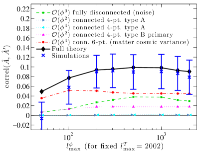
(a)

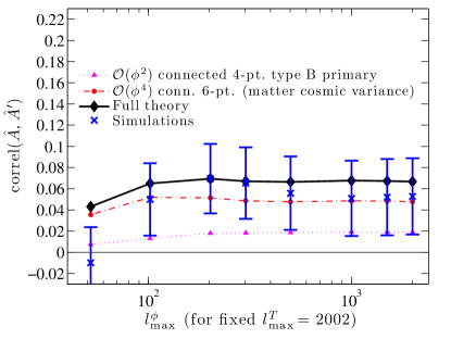
(b)

Figure 8: (a) Correlation $\mathrm{\widehat{correl}}(\hat{A},\hat{A}^{\prime})=\widehat{\mathrm{cov}}(\hat{A},\hat{A}^{\prime})/(\sigma_{A}\sigma_{A^{\prime}})$ of the lensing amplitude estimates of Eqs. (54) and (55) measured in $1000$ simulations (blue crosses), if no empirical $\hat{N}^{(0)}$ subtraction is applied. The theoretical correlation from Eq. (56) (black) includes the noise contribution of Eq. (35), the matter cosmic variance contribution of Eq. (111) and the dominant connected $4$-point contributions from Eqs. (100) and (102). In the simulations the lensing potential is reconstructed from the lensed temperature power spectrum up to $l_{\mathrm{max}}^{\mathrm{rec}}=2750$. Then, $\hat{A}$ is estimated from $\hat{C}_{l}^{\hat{\phi}\hat{\phi}}$ from $l^{\phi}_{\mathrm{min}}=2$ up to the multipole $l^{\phi}_{\mathrm{max}}$, which is varied along the horizontal axis. The amplitude $\hat{A}^{\prime}$ is estimated using $\hat{C}^{\tilde{T}\tilde{T}}_{l,\mathrm{expt}}$ up to $l_{\mathrm{max}}^{T}=2002$. Theoretical expressions are evaluated with the same cut-offs (non-diagonal covariance matrices are cut off before inverting them). Error bars show standard errors on the measured correlation. The errors are very correlated because they all involve overlapping low-$l$ reconstruction modes. (b) Same as (a) but with empirical $\hat{N}^{(0)}$ subtraction. Since this removes some covariance contributions, the theoretical covariance is given by Eqs. (102) and (111) only.

Instead of fixing $l^{\phi}_{\mathrm{min}}=2$ and varying $l^{\phi}_{\mathrm{max}}$ it is worthwhile to consider the disjoint reconstruction bins $[l^{\phi}_{\mathrm{min}},l^{\phi}_{\mathrm{max}}]=[40,84]$, $[85,129]$, $[130,174]$, $\dots$, $[355,400]$ used for the Planck analyses in Planck Collaboration et al. (2013b, a). If the realisation-dependent $\hat{N}^{(0)}$ is used, the theoretical correlation of the lensing amplitude estimated from one of these bins alone with the lensing amplitude estimated from the temperature power (for $l^{T}_{\mathrm{max}}=2002$) is $5\%$, $3.6\%$ and $2\%$ for the first three reconstruction bins, and decreases further for the remaining higher-$l$ bins. This is consistent with the correlations estimated from our $1000$ simulations. In particular, this result shows that the lensing amplitude estimated from the temperature power spectrum and the reconstruction amplitudes used in the Planck lensing likelihood Planck Collaboration et al. (2013a) are nearly uncorrelated, which justifies neglecting this correlation in the likelihood.

For experiments with superior noise and beam characteristics the matter cosmic variance contribution to the temperature-lensing power covariance does not change, but the lensing amplitude errors decrease. We therefore expect the corresponding amplitude correlation to increase. For example, for a full-sky experiment with SPT-like noise and beam specificiations, $\sigma_{N}=18\,\mu\mathrm{K}\,\mathrm{arcmin}$ and $\sigma_{\mathrm{FWHM}}=1\,\mathrm{arcmin}$, the amplitude correlation from the matter cosmic variance contribution alone is around $10$–$11\%$ for $l_{\mathrm{max}}^{T}=2002$ and $l_{\mathrm{max}}^{\phi}=500$–$1000$.

Combined lensing amplitude estimate

We have presented two estimators of the lensing amplitude: $\hat{A}$ is linear in the reconstruction power and $\hat{A}^{\prime}$ is linear in the CMB power. These two estimates can be combined with inverse variance weighting,

$$\hat{A}_{C}=\frac{1}{\sigma_{A}^{-2}+\sigma_{A^{\prime}}^{-2}}\left(\frac{\hat{A}}{\sigma_{A}^{2}}+\frac{\hat{A}^{\prime}}{\sigma_{A^{\prime}}^{2}}\right).$$ (59)

This combined estimator is the maximum-likelihood estimator for the lensing amplitude if $\hat{A}$ and $\hat{A}^{\prime}$ are assumed to be uncorrelated. If there is a correlation between $\hat{A}$ and $\hat{A}^{\prime}$ this does not change the expectation value of $\hat{A}_{C}$, but it does change its variance, which is then given by

$$\mathrm{var}(\hat{A}_{C})=\sigma_{A}\sigma_{A^{\prime}}\left(\frac{\sigma_{A}}{\sigma_{A^{\prime}}}+\frac{\sigma_{A^{\prime}}}{\sigma_{A}}\right)^{-2}\left[\left(\frac{\sigma_{A}}{\sigma_{A^{\prime}}}+\frac{\sigma_{A^{\prime}}}{\sigma_{A}}\right)+2\,\mathrm{correl}(\hat{A},\hat{A}^{\prime})\right].$$ (60)

A correlation between $\hat{A}$ and $\hat{A}^{\prime}$ therefore increases the $1\sigma$ error of the combined estimator (59) by a factor of

$$\frac{\sigma_{A_{C}}|_{\mathrm{cov}(A,A^{\prime})\neq 0}}{\sigma_{A_{C}}|_{\mathrm{cov}(A,A^{\prime})=0}}=\sqrt{1+\frac{2(\sigma_{A}/\sigma_{A^{\prime}})}{1+(\sigma_{A}/\sigma_{A^{\prime}})^{2}}\mathrm{correl}(\hat{A},\hat{A}^{\prime})}\leq\sqrt{1+\mathrm{correl}(\hat{A},\hat{A}^{\prime})}$$ (61)

compared to the error if $\hat{A}$ and $\hat{A}^{\prime}$ were uncorrelated. Since correlations between $\hat{A}$ and $\hat{A}^{\prime}$ were found to be at most $7\%$ if the empirical $\hat{N}^{(0)}$ subtraction is used, the $1\sigma$ error of the combined lensing estimate changes by at most $3.5\%$ for Planck ($5.5\%$ for the full-sky SPT-like experiment mentioned above). Noting that this is the error on the error bar, the correlations between $\hat{A}$ and $\hat{A}^{\prime}$ found above can be safely neglected when combining these two estimates of the lensing amplitude.

We briefly introduced a projection technique in Sec. V.2.5 to remove the covariance between the reconstructed lensing power and the lensed temperature power spectrum due to the cosmic variance of the lenses. A simple way to perform the projection is to modify the covariance matrix $(\text{cov}_{\hat{\phi}\hat{\phi}})_{ll^{\prime}}$ in Eq. (54) by adding $\lambda^{\prime}u_{l}u_{l^{\prime}}$, where $u_{l}$ is the dominant singular vector in Eq. (46), and taking $\lambda^{\prime}$ to infinity. To the extent that the covariance between the lensing and temperature power spectra is really rank-one, this procedure removes the correlation between $\hat{A}$ and $\hat{A}^{\prime}$ exactly. However, the variance of $\hat{A}$ is increased by projection: it is still given by Eq. (57) but with the modified $(\text{cov}_{\hat{\phi}\hat{\phi}})_{ll^{\prime}}$. For $l^{\phi}_{\mathrm{max}}=500$, we find that $\sigma_{A}$ is increased from $0.025$ to $0.042$, i.e. a 70% increase. This falls to 60% for $l^{\phi}_{\mathrm{max}}=1000$. The reason for the large increase is that $u_{l}$ is rather similar in shape to the signal whose amplitude we are trying to reconstruct. Given the large increase in the error on $\hat{A}$, and that ignoring the effect of the covariance between the lensing reconstruction and temperature power spectra is relatively harmless, we do not advocate the use of projection to remove the correlations.

V.4.2 Cosmological parameters

We naively expect the impact of power correlations on cosmological parameters to be smaller than for the lensing amplitude, because the latter is directly related to the lensing potential on all scales and can therefore accumulate contributions from the full power covariances. We confirm this with a simple Fisher analysis. The covariance matrix for the joint data vector $\underline{\hat{C}}=(\hat{C}^{\tilde{T}\tilde{T}}_{\mathrm{expt}},\hat{C}^{\hat{\phi}\hat{\phi}}-2\hat{N}^{(0)}+N^{(0)})$ is

$$\mathrm{cov}_{{LL^{\prime}},\,\mathrm{joint}}\equiv\mathrm{cov}(\underline{\hat{C}}_{L},\underline{\hat{C}}_{L^{\prime}})=\left(\begin{matrix}\delta_{LL^{\prime}}\mathrm{var}_{G}(C^{\tilde{T}\tilde{T}}_{L,\mathrm{expt}})&\mathrm{cov}(\hat{C}^{\tilde{T}\tilde{T}}_{L,\mathrm{expt}},\hat{C}^{\hat{\phi}\hat{\phi}}_{L^{\prime}}-2\hat{N}^{(0)}_{L^{\prime}})\\ \mathrm{cov}(\hat{C}^{\hat{\phi}\hat{\phi}}_{L}-2\hat{N}^{(0)}_{L},\hat{C}^{\tilde{T}\tilde{T}}_{L^{\prime},\mathrm{expt}})&\delta_{LL^{\prime}}\mathrm{var}_{G}(\langle\hat{C}_{L}^{\hat{\phi}\hat{\phi}}\rangle)\end{matrix}\right).$$ (62)

Fisher errors are obtained by taking the square root of the diagonal entries of the inverse of the Fisher matrix

$$F_{ij}=\sum_{LL^{\prime}}\frac{\partial\underline{C}_{L}}{\partial p_{i}}(\mathrm{cov}_{\mathrm{joint}}^{-1})_{LL^{\prime}}\frac{\partial\underline{C}_{L^{\prime}}}{\partial p_{j}}$$ (63)

for cosmological parameters $\mathbf{p}=(\Omega_{b}h^{2},\Omega_{c}h^{2},h,\tau,A_{s},n_{s},\Omega_{\nu}h^{2},\Omega_{K})$ and theoretical power spectra $\underline{C}=(C^{\tilde{T}\tilde{T}},C^{\phi\phi})$ (assuming cosmology-independent $N^{(0)}$ for simplicity). Including the off-diagonal temperature-lensing covariances of Eqs. (102) and (111) in Eq. (62) increases the Fisher errors for these parameters by at most $0.7\%$ ($0.5\%$ if only Eq. (111) is used) compared to a completely diagonal covariance matrix. The off-diagonal part of the joint covariance matrix can therefore safely be neglected for cosmological parameter estimation with a Planck-like experiment.

VI Towards a lensing likelihood

As argued in Sec. I, dealing with the exact likelihood for the lensed CMB temperature is generally computationally prohibitive. For this reason, we have focussed on a form of data compression whereby the non-Gaussian lensed CMB is represented by its 2- and 4-point functions (the latter via the lensing reconstrucion power spectrum). In computing the correlations between these spectra, we have implicitly been assuming that the likelihood takes the form of a multi-variate Gaussian in the spectra. In this section, we test the accuracy of this assumption in simple parameter-estimation exercises.

VI.1 Lensing amplitude from lensing reconstruction

As a toy model, we first aim to constrain the lensing amplitude $A$ from the lensing reconstruction alone. Considering an isotropic CMB survey, with Planck-like noise as described earlier, we consider two simple models for the likelihood, both of which depend only on the empirical power spectrum of the reconstruction. The first is the usual isotropic likelihood for a Gaussian field:

$$-2\ln\mathcal{L}_{1}(\hat{\phi}|A)=\sum_{l}(2l+1)\left(\frac{\hat{C}_{l}^{\hat{\phi}\hat{\phi}}}{AC_{l}^{\phi\phi}+N_{l}}+\ln\big{|}AC_{l}^{\phi\phi}+N_{l}|\right)+(\text{const.})\,.$$ (64)

This would be correct if $\hat{\phi}$ were a Gaussian field. However, since the reconstruction is manifestly non-Gaussian, we do not expect this likelihood to perform well. The second is Gaussian in the empirical power spectrum $\hat{C}^{\hat{\phi}\hat{\phi}}$:

$$-2\ln\mathcal{L}_{2}(\hat{C}^{\hat{\phi}\hat{\phi}}|A)=\sum_{l,l^{\prime}}\left[\hat{C}_{l}^{\hat{\phi}\hat{\phi}}-(AC_{l}^{\phi\phi}+N_{l})\right](\mathrm{cov}_{\hat{\phi}\hat{\phi}}^{-1})_{ll^{\prime}}\left[\hat{C}_{l^{\prime}}^{\hat{\phi}\hat{\phi}}-(AC_{l^{\prime}}^{\phi\phi}+N_{l^{\prime}})\right]+(\text{const.})\,.$$ (65)

The theoretical reconstruction power auto-covariance $\mathrm{cov}_{\hat{\phi}\hat{\phi}}$, given by Eqs. (28) and (29), and the bias of the reconstructed lensing power, $N=N^{(0)}+N^{(1)}$, are evaluated for the fiducial amplitude $A=1$. The empirical $\hat{N}^{(0)}$ subtraction is obtained by replacing $N$ with $\hat{N}=2\hat{N}^{(0)}-N^{(0)}+N^{(1)}$. For $\mathcal{L}_{1}$, the maximum-likelihood estimate for $A$ (given a realisation of the lensing reconstruction) is found numerically by direct evaluation of $\mathcal{L}_{1}$ for various $A$. The maximum likelihood estimator for $A$ based on the second likelihood $\mathcal{L}_{2}$ is given by Eq. (54).

We compute estimates $\hat{A}$ of the lensing amplitude for $1000$ realisations of the lensed CMB. The sample mean of $\hat{A}$ should be unity and the sample variance of $\hat{A}$, i.e. the scatter of the best-fit amplitude over different realisations, should agree with the typical width of the likelihood evaluated for a single realisation. Checking these two properties provides a non-trivial test of the likelihood $\mathcal{L}_{1}$. In contrast, for $\mathcal{L}_{2}$, rather than testing the accuracy of $\mathcal{L}_{2}$, the sample mean and sample variance of $\hat{A}$ just test our understanding of the mean and covariance of $\hat{C}^{\hat{\phi}\hat{\phi}}$. This test is still useful to check for residual biases and the accuracy of our model for the reconstruction power covariance.

Figure 9 compares the likelihood evaluated for several individual realisations (coloured) with a Gaussian (black) with mean and standard deviation given by sample mean and standard deviation of $\hat{A}$ averaged over all $1000$ realisations (for $l_{\mathrm{max}}^{\phi}=2650$ and our Planck-like noise model). Including the $N^{(1)}$ bias is important at high multipoles for both likelihoods: e.g. without it, $\mathcal{L}_{1}$ overestimates the lensing amplitude by $9\%$; see Fig. 9a. Including the $N^{(1)}$ bias in $\mathcal{L}_{1}$ yields the correct lensing amplitude $A=1$ in the mean, but the scatter of $\hat{A}$ over realisations is more than $30\%$ larger than the typical width of $\mathcal{L}_{1}$ in a single realisation; see Fig. 9b. The likelihood $\mathcal{L}_{1}$ underpredicts the error of $A$ because of the non-Gaussianity of $\hat{\phi}$. This is demonstrated in Fig. 9c, for which we replace the reconstructions with Gaussian simulations of a field with power spectrum $C_{l}^{\phi\phi}+N_{l}^{(0)}+N_{l}^{(1)}$. In this case, $\mathcal{L}_{1}$ should be exact and the scatter does indeed match the widths of individual realisations.

In contrast, $\mathcal{L}_{2}$ can partly model the non-Gaussianity of $\hat{\phi}$ through the non-diagonal reconstruction power auto-covariance. We compute $\hat{A}$ based on $\mathcal{L}_{2}$ for different forms of the lensing covariance. Neglecting off-diagonal contributions to $\mathrm{cov}_{\hat{\phi}\hat{\phi}}$ gives likelihood-based errors for $A$ less than $80\%$ of the scatter of $\hat{A}$ across the simulations; see Fig. 9d. If we include non-Gaussian, off-diagonal contributions given by Eq. (28), we find that $\mathcal{L}_{2}$ predicts the scatter in $A$ to better than $5\%$; see Fig. 9e. Similar results are achieved with the empirical $\hat{N}^{(0)}$ correction of Eq. (17) and diagonal (Gaussian) reconstruction power covariance; see Fig. 9f.

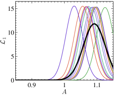
(a)

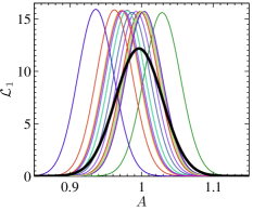
(b)

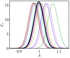
(c)

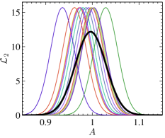
(d)

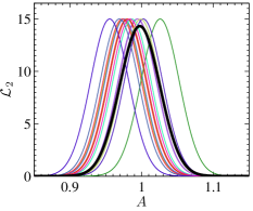
(e)

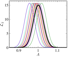
(f)

Figure 9: Likelihoods for the lensing amplitude for $15$ different realisations (thin, coloured lines), using the lensing reconstruction up to $l_{\mathrm{max}}^{\phi}=2650$, compared with the scatter in the best-fit amplitude obtained over 1000 simulations. Each likelihood peaks at some best-fit parameter $\hat{A}$, and the mean and scatter of these best-fitting amplitudes over all 1000 simulations correspond to the Gaussian curves (thick black). The upper panels show $\mathcal{L}_{1}$ from Eq. (64), while the lower panels show $\mathcal{L}_{2}$ given by Eq. (65). All curves are normalised such that their integral over $A$ is unity.

VI.2 Two-parameter likelihood tests with lensing amplitude and lensing tilt

To test the likelihood approximation $\mathcal{L}_{2}$ we use the lensing reconstruction additionally to constrain the lensing tilt $n$ defined by

$$C_{l}^{\phi\phi}=A\left(\frac{l}{l_{*}}\right)^{n}C_{l}^{\phi\phi}|_{\mathrm{fid}}.$$ (66)

The pivot multipole $l_{*}=124$ is chosen such that the Fisher matrix associated with $\mathcal{L}_{2}$ is diagonal [for $l_{\mathrm{max}}^{\phi}=\mathcal{O}(10^{3})$], implying that the parameters $A$ and $n$ are approximately uncorrelated. The likelihoods for nine realisations are compared with the scatter of the best-fit parameters over $1000$ realisations in Fig. 10. If the non-diagonal lensing power covariance of Eq. (28) is included we find good agreement (without empiricial $\hat{N}^{(0)}$ subtraction). Note that we have binned the reconstruction power in bins with boundaries at

$$l=2,13,35,75,115,155,195,\dots\quad\mbox{(increasing by $40$ above $l=35$)}.$$ (67)

Similar results for the unbinned case will be summarised in Fig. 11 below.

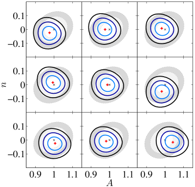
(a)

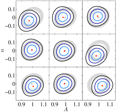
(b)

Figure 10: Likelihood test if lensing amplitude $A$ (horizontal axis) and tilt $n$ (vertical axis) are varied. Thick lines: Contours enclosing $68\%$, $95\%$ and $99.7\%$ of the probability for the likelihood $\mathcal{L}_{2}$ (65) evaluated for nine realisations. Gray filled ellipses: Contours of a Gaussian with central point and covariance matrix estimated from the scatter of the best-fit parameters over 1000 realisations. The lensing power auto-covariance $\mathrm{cov}_{\hat{\phi}\hat{\phi}}$ is assumed to be diagonal in (a), while (b) also includes the non-diagonal contribution in Eq. (28). The reconstruction power is used up to $l_{\mathrm{max}}^{\phi}=1002$ and is binned as described in the text.

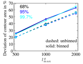
(a)

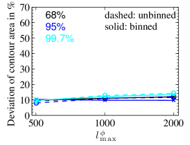
(b)

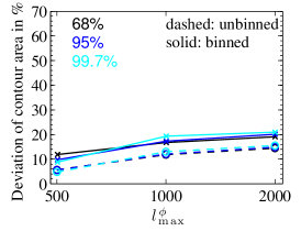
(c)

Figure 11: Quantitative comparison of areas in the $A$ vs. $n$ plane enclosed by contours of the $\mathcal{L}_{2}$ likelihood. We show the fractional deviation of the areas of Gaussians (with sample mean and sample covariance derived from the scatter of the best fit-parameters over 1000 realisations) from the average area in a single realisation. Positive values mean that the width of the likelihood typically underestimates the scatter of its peak across realisations. Results are shown for unbinned power spectra (dashed lines) and power spectra binned according to the scheme of Eq. (67) (solid lines); and for $68\%$ (black), $95\%$ (blue) and $99.7\%$ (cyan) confidence levels. The maximum multipole of the reconstruction power is varied along the horizontal axis (only for three values which are connected by straight lines to guide the eye). The lensing power auto-covariance $\mathrm{cov}_{\hat{\phi}\hat{\phi}}$ in $\mathcal{L}_{2}$ is assumed to be diagonal in (a), while (b) also includes the non-diagonal contribution of Eq. (28). Panel (c) is for empirical $\hat{N}^{(0)}$ bias correction and diagonal covariance. The contours in Fig. 10 correspond to the crosses at $l^{\phi}_{\mathrm{max}}=1002$ in (a) and (b).

To quantify the level of agreement between the likelihoods for individual realisations and the scatter of their best-fit parameters, we compare the areas of the confidence contours shown in Fig. 10. We show in Fig. 11 the fractional deviation of the areas of the Gaussian, with sample mean and sample covariance matched to the scatter of the best-fit parameters over realisations, from the average area of the likelihoods for individual realisations (i.e. the fractional deviation of gray background areas from average areas enclosed by the solid lines in Fig. 10).

Neglecting the off-diagonal contribution to the lensing power covariance, which is largest at high reconstruction multipoles Hanson et al. (2011), gives narrow misshapen likelihoods that underestimate the scatter across simulations. This is particularly so for $l_{\mathrm{max}}^{\phi}\gtrsim 1000$ where the confidence areas disagree by around $40$–$65\%$. Binning does not help because it does not reduce the broad-band correlations of the reconstruction power. The agreement is better when the non-diagonal reconstruction power covariance is used (the disagreement of confidence areas is at most $14\%$). Alternatively, if the empirical $\hat{N}^{(0)}$ bias correction and the diagonal covariance is used, the confidence areas deviate by at most $22\%$. If we assume circular contours the fractional deviation of the contour radius is $\sqrt{1+d}-1<d/2$ if $d$ is the fractional deviation of the contour areas. Taking this as the approximate fractional error of the marginalised error bars of $A$ or $n$ shows that the error on the error bars is smaller than $11\%$ if the non-diagonal reconstruction covariance or empirical $\hat{N}^{(0)}$ subtraction are used in $\mathcal{L}_{2}$. Therefore these two cases provide a reasonably accurate model for the lensing likelihood in this test. If diagonal reconstruction power covariance is assumed, and no empirical $\hat{N}^{(0)}$ subtraction performed, the error on the error bars can reach $30\%$ even if binning is used. It is also worth noting that in this last case only the confidence areas increase with $l^{\phi}_{\mathrm{max}}$, i.e. the analysis is clearly non-optimal.

Note that in the above, ideally, we should use a histogram of the best-fit parameters instead of fitting a Gaussian to their scatter. This would test the tails of the distribution much better because it would include possible skewness etc. However we find that histograms from $1000$ simulations are too noisy to be useful for this purpose, giving results that scatter significantly with changes in histogram binning widths $\Delta A$ and $\Delta n$.

VII Conclusions

To include the CMB lensing reconstruction power spectrum in a joint likelihood analysis with the power spectrum of the temperature anisotropies requires knowledge of the cross-covariance of the two spectra. We computed this cross-covariance between the CMB 4-point and 2-point functions perturbatively, identifying two physical contributions. The disconnected part of the $6$-point function of the lensed temperature leads to a noise contribution which can be interpreted as the response of the statistical noise in the lens reconstruction to fluctuations in the underlying CMB temperature field. The connected $\mathcal{O}(\phi^{4})$ piece of the $6$-point function gives rise to a second contribution attributable to the cosmic variance of the lenses, which causes the power spectrum of the lens reconstruction and the smoothing effect in the anisotropy power spectrum to covary. The temperature-lensing power covariance can therefore be written as

$$\mathrm{cov}(\hat{C}^{\hat{\phi}\hat{\phi}}_{L},\hat{C}^{\tilde{T}\tilde{T}}_{L^{\prime},\mathrm{expt}})\;=\;\frac{\partial(2\hat{N}^{(0)}_{L})}{\partial\hat{C}^{\tilde{T}\tilde{T}}_{L^{\prime},\mathrm{expt}}}\;\frac{2}{2L^{\prime}+1}(C^{\tilde{T}\tilde{T}}_{L^{\prime},\mathrm{expt}})^{2}\left[1+2\frac{C^{\phi\phi}_{L}}{A_{L}}\right]\;+\;\frac{2}{2L+1}(C^{\phi\phi}_{L})^{2}\;\frac{\partial C^{\tilde{T}\tilde{T}}_{L^{\prime}}}{\partial C^{\phi\phi}_{L}},$$ (68)

where perturbative expressions for the derivatives are given in Eqs. (27) and (31). Both contributions were confirmed with simulations. The second term in the square brackets represents the leading correction from the connected 4-point function; see Eq. (102). The $C^{T\phi}$ correlation gives a diagonal contribution to the temperature-lensing power correlation, which is less than $5\%$ for Planck-like specifications and falls rapidly with $L$. This generally has a negligible impact on parameter constraints derived jointly from the CMB 2- and 4-point functions.

We showed that correcting for the Gaussian $N^{(0)}$ bias in the reconstruction power with the data-dependent $\hat{N}^{(0)}$, advocated by Hanson et al. (2011) to remove auto-covariances of the lensing reconstruction power spectrum, also removes the noise contribution to the temperature-lensing power correlation and we provided an intuitive interpretation of this result.

For Planck-like specifications, estimates of the lensing amplitude $A$ based on the lensing reconstruction or the peak smearing of the lensed temperature power spectrum can be correlated at around the $10\%$ level due to the power correlations. If the correlations are ignored, this gives a mis-estimate of the error on a joint amplitude estimate of only $5\%$, which should be negligible. The data-dependent $\hat{N}^{(0)}$ bias correction reduces the amplitude correlation further to $7\%$ and the error of the error to $3.5\%$. Intuitively, we can understand the smallness of the correlation (found perturbatively and with simulations) by noting that: (i) covariance of the amplitude estimates due to cosmic variance of the lenses is limited by the small number of modes of $C^{\phi\phi}$ that influence the acoustic region of the temperature power spectrum, and is diluted significantly by CMB cosmic variance (and noise); and (ii) roughly disjoint scales in the CMB contribute to the amplitude determination from peak smearing and to the lens reconstruction limiting the correlation due to CMB cosmic variance. (See Appendix A for further details of these arguments.) For a joint analysis of the power spectrum of a temperature-based CMB lensing reconstruction and the power spectrum of the temperature anisotropies themselves, the likelihoods for these two observables can therefore be simply combined for a Planck-like experiment (as was the case for the 2013 Planck analysis Planck Collaboration et al. (2013a)).

Non-Gaussianity of the lensing reconstruction complicates the construction of a likelihood. We showed that the usual likelihood for isotropic Gaussian fields does not perform well for lens reconstruction in simple parameter tests, significantly underestimating the scatter seen in the best-fitting parameters across simulations. We obtained better results with simple likelihoods that are Gaussian in the measured spectra (with fiducial covariance matrix) provided that power spectrum covariances were properly modeled or data-dependent $N^{(0)}$ subtraction included. In two-parameter tests based on the amplitude and tilt of a fiducial lensing power spectrum, the widths of these Gaussian likelihoods reproduce the scatter in parameters across simulations at the $10\%$ level.

With polarization-based reconstructions becoming feasible with current observations, it will be important to extend the analysis presented here to polarization (see Zahn et al. (2013) for work in this direction). While we expect that many of our results can be simply applied to reconstructions based on the temperature and polarization, the correlations are likely to be much more significant and particularly so for the most powerful $EB$-based reconstructions. We leave this to future work.

Appendix A Why are the lensing amplitude cross-correlations so small?

The calculations in this paper give a rigorous derivation of the cross-correlation of the power spectra of the lensing reconstruction and the temperature anisotropies. In this appendix we present simple physical arguments for why the correlation of the lensing amplitudes estimated from the reconstruction power and the anisotropy power are so small. We present these arguments first for the correlation due to CMB cosmic variance and then for the correlation due to cosmic variance of the lenses.

A.1 Cosmic variance of the CMB

Due to the smoothing effect of lensing, most of the constraint on the lensing amplitude $\hat{A}^{\prime}$ estimated from the CMB power spectrum comes from the CMB on scales of the acoustic peaks and troughs. This can be seen directly from the contribution $s_{l}^{\tilde{T}\tilde{T}}$ to the total signal-to-noise squared [$(S/N)^{2}$] associated with the CMB cosmic variance at multipole $l$ (see the blue curve in Fig. 12):

$$\left(\frac{S}{N}\right)_{A^{\prime}}^{2}=\frac{1}{\sigma_{A^{\prime}}^{2}}=\sum_{l=l_{\mathrm{min}}^{T}}^{l_{\mathrm{max}}^{T}}\underbrace{\frac{(C_{l}^{\tilde{T}\tilde{T}}-C_{l}^{TT})^{2}}{\text{var}_{G}(C^{\tilde{T}\tilde{T}}_{l,\mathrm{expt}})}}_{s_{l}^{\tilde{T}\tilde{T}}}.$$ (69)

In contrast, in the limit of very large-scale lenses, and as argued in more detail below, the reconstruction combines local convergence and shear measurements, for which scales in the CMB where the power spectrum changes rapidly are most informative. For large-scale lenses, the $(S/N)^{2}$ on the reconstruction-based amplitude estimate $\hat{A}$ is thus expected to be dominated by CMB modes between acoustic peaks and troughs. Therefore, the lensing amplitude estimates $\hat{A}$ and $\hat{A}^{\prime}$ are determined by rather disjoint CMB modes with independent CMB cosmic-variance fluctuations. We therefore expect the amplitude correlation due to CMB cosmic variance to be suppressed (in case this correlation is not mitigated by the empirical $\hat{N}^{(0)}$ subtraction anyway).

To make this point more quantitative, note that the reconstruction power $\hat{C}^{\hat{\phi}\hat{\phi}}$ is affected by CMB cosmic variance through the disconnected CMB $4$-point contribution $N^{(0)}$. Keeping the estimator normalisation $A_{L}$ and weights $\tilde{g}$ fixed in Eq. (16), the contribution from the CMB at multipole $l$ to the $(S/N)^{2}$ of the reconstruction-based amplitude estimate $\hat{A}$ is monitored by

$$s_{l}^{\hat{\phi}\hat{\phi}}=\left|\frac{\delta\sigma_{A}^{-2}}{\delta\ln C^{\tilde{T}\tilde{T}}_{l,\mathrm{expt}}}\right|_{\text{fix}\,A_{L},\tilde{g}}=\sum_{L=l_{\mathrm{min}}^{\phi}}^{l_{\mathrm{max}}^{\phi}}\Bigg{|}\frac{-2(C_{L}^{\phi\phi})^{2}}{\frac{2}{2L+1}\big{(}N_{L}^{(0)}+C_{L}^{\phi\phi}+N_{L}^{(1)}\big{)}^{3}}\,\frac{4A_{L}^{2}}{2L+1}\sum_{l_{1}}\tilde{g}^{2}_{l_{1}l}(L)C^{\tilde{T}\tilde{T}}_{l_{1},\mathrm{expt}}\Bigg{|}C^{\tilde{T}\tilde{T}}_{l,\mathrm{expt}},$$ (70)

where we used $\sigma_{A}$ from Eq. (57) and kept only the dominant diagonal part of the reconstruction power auto-covariance. As shown in Fig. 12, $s_{l}^{\hat{\phi}\hat{\phi}}$ (red) is out of phase compared to $s_{l}^{\tilde{T}\tilde{T}}$ (blue). To understand this structure, we separate the sums over $L$ and $l_{1}$ in Eq. (70) by restricting ourselves to very large-scale lenses, $l^{\phi}_{\mathrm{max}}\ll l$, and using the large scale approximation for $N^{(0)}$ derived in Hanson et al. (2011) [see their Eq. (19)], to find

$$s_{l}^{\hat{\phi}\hat{\phi}}\approx s^{\hat{\phi}\hat{\phi}}_{l,\text{approx}}=f(l^{\phi}_{\mathrm{min}},l^{\phi}_{\mathrm{max}})\frac{1}{\text{var}_{G}(C^{\tilde{T}\tilde{T}}_{l,\mathrm{expt}})}\left[\left(C^{\tilde{T}\tilde{T}}_{l}\frac{\mathrm{d}\ln(l^{2}C^{\tilde{T}\tilde{T}}_{l})}{\mathrm{d}\ln l}\right)^{2}+\frac{1}{2}\left(C^{\tilde{T}\tilde{T}}_{l}\frac{\mathrm{d}\ln C^{\tilde{T}\tilde{T}}_{l}}{\mathrm{d}\ln l}\right)^{2}\right],\quad[l^{\phi}_{\mathrm{max}}\lesssim\mathcal{O}(10)].$$ (71)

Here, the prefactor $f$ depends on the minimum and maximum reconstruction multipole but not on the CMB multipole $l$. The terms in square brackets have the form of the quadrature sum of the information in convergence and shear. Convergence changes locally the angular scale of the CMB anisotropies and so would contribute nothing to the $(S/N)^{2}$ for a scale-invariant spectrum, $l^{2}C_{l}=\text{const.}$, while shear contributes nothing for a white-noise spectrum, $C_{l}=\text{const}$. Thus, for large-scale lenses, the $(S/N)^{2}$ for the reconstruction-based amplitude gets most contributions from CMB scales where the gradient of the CMB power spectrum is maximal, i.e. between acoustic peaks and troughs (see red and black curves in Fig. 12a).

In reality, temperature multipoles that are not precisely at peaks or troughs and not precisely in between them will affect both amplitude estimates, which implies a small amplitude correlation. Intermediate- and small-scale lenses can mix CMB modes over multipole ranges comparable to the acoustic peak separation so that they are affected by wider ranges of CMB multipoles than argued above (see red curve in Fig. 12b), which implies a somewhat larger amplitude correlation. However, since the CMB scales that are most important for the reconstruction still have negligible impact on the amplitude estimated from the temperature power, we expect the correlation of the amplitudes to stay rather small.

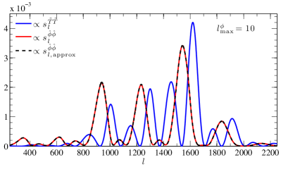
(a)

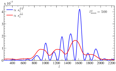
(b)

Figure 12: Contribution of different CMB multipoles $l$ to the $(S/N)^{2}$ of the lensing amplitude for estimators based on the CMB power spectrum [blue; Eq. (69)] and on the lensing reconstruction [red; Eq. (70)] for $l^{\phi}_{\mathrm{max}}=10$ (left) and $l^{\phi}_{\mathrm{max}}=500$ (right). The approximation in Eq. (71) for large-scale lenses is shown in black dashed in the left plot. Since we are not interested in the total $S/N$ but only in its distribution over different CMB scales, all curves are normalised such their integral over $l$ is unity.

A.2 Cosmic variance of the lenses

We now consider the contribution of cosmic variance of the lenses to the covariance of the lensing amplitude estimates given in Eq. (56). It is instructive to consider a toy-model where the reconstruction “noise” power is proportional to $C^{\phi\phi}$, i.e. $N_{l}^{(0)}+N_{l}^{(1)}=\lambda C_{l}^{\phi\phi}$. Taking the limit $\lambda\rightarrow 0$ is equivalent to being able to observe $\phi$ directly with no measurement error, while $\lambda\rightarrow\infty$ corresponds to there being no information in the reconstruction. With $N_{l}^{(0)}+N_{l}^{(1)}=\lambda C_{l}^{\phi\phi}$, the weighting of the reconstruction power spectrum in $\hat{A}$ is the same as for an ideal reconstruction (i.e. one with no $N^{(0)}$ and $N^{(1)}$ noise). Provided we then determine $\hat{A}$ from all those $\phi$ modes that influence the temperature power spectrum, the contribution to the amplitude covariance from cosmic variance of the lenses simplifies significantly to give

$$\text{cov}(\hat{A},\hat{A}^{\prime})=\sigma_{A,\text{ideal}}^{2}.$$ (72)

Here, $\sigma_{A,\text{ideal}}^{2}=[\sum_{l}(l+1/2)]^{-1}\approx 2/(l_{\text{max}}^{\phi})^{2}$ is the variance of the reconstruction-based amplitude in the ideal limit $\lambda\rightarrow 0$ using all modes up to $l_{\text{max}}^{\phi}$. Since only a few (large-scale) lensing modes affect $\hat{A}^{\prime}$, including more lensing modes in the reconstruction dilutes the covariation of $\hat{A}$ and $\hat{A}^{\prime}$ over different realisations of the lenses, because there are increasingly more lensing modes in $\hat{A}$ whose fluctuations do not enter $\hat{A}^{\prime}$. The amplitude covariance falls inversely as the number of modes in the reconstruction since the weight in $\hat{A}$ given to those (few) modes of $C^{\phi\phi}$ that influence the temperature power spectrum falls as the total number of modes. Note that the covariance is independent of the weighting of the measured temperature power spectrum in $\hat{A}^{\prime}$, provided $\hat{A}^{\prime}$ is appropriately normalised, and it is also independent of additional contributions to the reconstruction noise (e.g. from CMB cosmic variance, for fixed $l^{\phi}_{\text{max}}$). The variance of $\hat{A}$ does depend on the reconstruction noise level, with

$$\sigma_{A}^{-2} \approx \sum_{l}\frac{2l+1}{2}\left(\frac{C_{l}^{\phi\phi}}{C_{l}^{\phi\phi}+N_{l}^{(0)}+N_{l}^{(1)}}\right)^{2}$$ (73)

$$= \frac{1}{(1+\lambda)^{2}}\sum_{l}\frac{2l+1}{2}=\frac{1}{(1+\lambda)^{2}}\sigma_{A,\text{ideal}}^{-2}.$$

The result $\text{cov}(\hat{A},\hat{A}^{\prime})=\sigma_{A,\text{ideal}}^{2}$ for ideal weighting is necessary to ensure that the lensed CMB spectrum adds no further information on the lensing amplitude when combined with an ideal measurement of $\phi$ itself on all scales that are relevant for peak smearing of the temperature power spectrum. To see this, note that we can combine the amplitude estimates $\hat{A}$ and $\hat{A}^{\prime}$ optimally into a single estimate $\hat{A}_{\text{opt.}}$, properly taking account of their correlation. If we do this, the inverse variance of the optimal estimate is given by contracting the inverse covariance matrix of the estimates:

$$\sigma_{A,\text{opt.}}^{-2}=\text{cov}^{-1}(\hat{A},\hat{A})+2\,\text{cov}^{-1}(\hat{A},\hat{A}^{\prime})+\text{cov}^{-1}(\hat{A}^{\prime},\hat{A}^{\prime}).$$ (74)

This evaluates to

$$\sigma_{A,\text{opt.}}^{-2}=\frac{\sigma_{A}^{2}+\sigma^{2}_{A^{\prime}}-2\sigma^{2}_{A,\text{ideal}}}{\sigma_{A}^{2}\sigma^{2}_{A^{\prime}}-\sigma_{A,\text{ideal}}^{4}},$$ (75)

on using Eq. (72) for the covariance. In the ideal case, taking the limit $\lambda\rightarrow 0$, we have $\sigma_{A}=\sigma_{A,\text{ideal}}$ so that $\sigma_{A,\text{opt}.}=\sigma_{A,\text{ideal}}$. This as it must be – the observation of the peak smearing in the power spectrum adds no new information to that obtained from the ideal measurement of $\phi$. In the opposite limit, $\lambda\rightarrow\infty$, we have $\sigma_{A}\rightarrow\infty$ and $\sigma_{A,\text{opt.}}=\sigma_{A^{\prime}}$ and all information is coming from the temperature power spectrum.

The correlation induced by matter cosmic variance,

$$\text{correl}(\hat{A},\hat{A}^{\prime})=\frac{\sigma^{2}_{A,\text{ideal}}}{\sigma_{A}\sigma_{A^{\prime}}}=\frac{\sigma_{A}}{(1+\lambda)^{2}\sigma_{A^{\prime}}},$$ (76)

reaches its maximal value of $\sigma_{A,\text{ideal}}/\sigma_{A^{\prime}}$ if the variance of the reconstruction power spectrum is only due to matter cosmic variance, $\lambda=(N_{L}^{(0)}+N_{L}^{(1)})/C_{L}^{\phi\phi}\rightarrow 0$; and it falls monotonically with increasing $\lambda$, tending to zero as $\lambda\rightarrow\infty$ (when CMB cosmic variance dominates the reconstruction uncertainty). This is expected since we assume matter and CMB fluctuations to be independent. More generally, $\sigma_{A}$ is determined by the number of high $S/N$ modes in the reconstruction, but $\sigma_{A^{\prime}}$ depends not only on the number of CMB modes but also the fractional size of the power spectrum corrections from lensing relative to the total spectrum, $C_{l,\text{expt}}^{\tilde{T}\tilde{T}}$. The result is that both factors $\sigma_{A,\text{ideal}}/\sigma_{A}$ and $\sigma_{A,\text{ideal}}/\sigma_{A^{\prime}}$ in Eq. (76) are less than $1$, diluting the amplitude correlation.

For our Planck-like parameters, the power spectrum corrections from lensing are only ever a few percent of the total spectrum and so cosmic variance of the CMB limits $\sigma_{A^{\prime}}\approx 0.04$. Statistical noise in the lens reconstruction limits $\sigma_{A}\approx 0.025$. It is clear from Fig. 1 that a constant $\lambda$ is not a good approximation for lens reconstruction, but we can crudely limit $\lambda\gtrsim 2$ in which case we expect the amplitude correlation to be less than $(0.025/0.04)/3^{2}\sim 0.06$ which is close to the value plotted in Fig. 8.

To summarise, the correlation of the lensing amplitudes due to the cosmic variance of the lenses is generally small since there are a limited number of modes of $C^{\phi\phi}$ that influence the acoustic part of the temperature power spectrum (so the covariance for an ideal reconstruction scales inversely as the number of reconstruction modes), and the small covariance [less than $O(10^{-4})$] is diluted by cosmic variance of the CMB (and noise), which dominates the error on $\hat{A}^{\prime}$ and contributes significantly to the error on $\hat{A}$. We emphasise that these conclusions assume that the temperature power spectrum at multipoles $l\gtrsim 3000$, where the lensing-induced power from small-scale lenses dominates the unlensed power, does not influence the amplitude estimate (i.e. the spectrum is limited by noise or foregrounds there).

Appendix B Optimal trispectrum estimation and $N^{(0)}$ subtraction

In this appendix we show that the lensing power spectrum estimator advocated in Sec. II, which includes a data-dependent $N^{(0)}$ subtraction to remove the (disconnected) Gaussian bias, follows naturally from optimal trispectrum estimation (e.g. Regan et al. (2010)). Moreover, we show that in the Gaussian limit, this estimator is uncorrelated with any quadratic estimate of the temperature power spectrum, generalising the result established in Sec. V.1.4.

We start by considering the Gram-Charlier expansion for the probability density function (PDF) of a weakly non-Gaussian, zero-mean temperature field $T$. Writing the field in an arbitrary basis (e.g. a pixelised map or multipole coefficients) as $T_{i}$, with covariance $\langle T_{i}T_{j}\rangle=C_{ij}$, the expansion truncated at the trispectrum level can be written in the form Regan et al. (2010)

$$P(T) = \frac{e^{-T_{i}C_{ij}^{-1}T_{j}/2}}{\sqrt{\mathrm{det}(2\pi C)}}\biggl{(}1+\frac{1}{24}\langle T_{i}T_{j}T_{k}T_{l}\rangle_{c}\bigl{(}\bar{T}_{i}\bar{T}_{j}\bar{T}_{k}\bar{T}_{l}-[C_{ij}^{-1}\bar{T}_{k}\bar{T}_{l}+C^{-1}_{kl}\bar{T}_{i}\bar{T}_{j}-C^{-1}_{ij}C^{-1}_{kl}]$$ (77)

$$\mbox{}\hskip 86.72267pt-[C_{ik}^{-1}\bar{T}_{j}\bar{T}_{l}+C^{-1}_{jl}\bar{T}_{i}\bar{T}_{k}-C^{-1}_{ik}C^{-1}_{jl}]-[C_{il}^{-1}\bar{T}_{j}\bar{T}_{k}+C^{-1}_{jk}\bar{T}_{i}\bar{T}_{l}-C^{-1}_{jk}C^{-1}_{il}]\bigr{)}\biggr{)}.$$

Here, $\bar{T}_{i}\equiv C_{ij}^{-1}T_{j}$ is the field filtered by the inverse covariance and summation over repeated indices is implicit. Note that $\langle\bar{T}_{i}\bar{T}_{j}\rangle=C_{ij}^{-1}$. We have ignored bispectrum contributions (due to the lensing-ISW correlation) which is a good approximation on intermediate and small scales. Using Wick’s theorem, it is straightforward to show from Eq. (77) that the mean and bispectrum of $T$ vanish, whilst the covariance is $C_{ij}$ and the trispectrum is $\langle T_{i}T_{j}T_{k}T_{l}\rangle_{c}$, as intended. That the covariance is $C_{ij}$ implies that the data combination associated with the trispectrum term in Eq. (77) is orthogonal to any quadratic function of $T$ with respect to the Gaussian weight function. In other words, if $T$ were Gaussian, this data combination is uncorrelated with any quadratic function of $T$.

We can form an estimator for $C_{L}^{\phi\phi}$ by maximising the PDF with respect to $C_{L}^{\phi\phi}$. In practice, we can approximate this by one step of a Newton-Raphson scheme starting at $C_{L}^{\phi\phi}=0$. The estimator is then proportional to $\partial\ln P(T)/\partial C_{L}^{\phi\phi}$ evaluated at $C_{L}^{\phi\phi}=0$. The lensing power spectrum enters the PDF explicitly through the connected 4-point function, and also implicitly through the lensed $\tilde{C}_{l}^{TT}$ in the covariance $C_{ij}$. The contribution to the $C_{L}^{\phi\phi}$ estimate from the 4-point function is of the form

$$\hat{C}_{L}^{\phi\phi} \sim \frac{\partial}{\partial C_{L}^{\phi\phi}}\langle T_{i}T_{j}T_{k}T_{l}\rangle_{c}\bigl{(}\bar{T}_{i}\bar{T}_{j}\bar{T}_{k}\bar{T}_{l}-[C_{ij}^{-1}\bar{T}_{k}\bar{T}_{l}+C^{-1}_{kl}\bar{T}_{i}\bar{T}_{j}-C^{-1}_{ij}C^{-1}_{kl}]$$ (78)

$$\mbox{}\hskip 85.35826pt-[C_{ik}^{-1}\bar{T}_{j}\bar{T}_{l}+C^{-1}_{jl}\bar{T}_{i}\bar{T}_{k}-C^{-1}_{ik}C^{-1}_{jl}]-[C_{il}^{-1}\bar{T}_{j}\bar{T}_{k}+C^{-1}_{jk}\bar{T}_{i}\bar{T}_{l}-C^{-1}_{jk}C^{-1}_{il}]\bigr{)}.$$

The terms involving the data in this equation are symmetric under permutations and so we need retain only primary couplings of the trispectrum, i.e., the first term in Eq. (13). The primary coupling has the form

$$\frac{\partial}{\partial C_{L}^{\phi\phi}}\langle T_{i}T_{j}T_{k}T_{l}\rangle_{c}^{\mathrm{primary}}\propto\sum_{M}(-1)^{M}X_{LM}^{ij}X_{L-M}^{kl},$$ (79)

where, in multipole space,

$$X_{LM}^{l_{1}m_{1}\,l_{2}m_{2}}=\tilde{f}_{l_{1}Ll_{2}}\left(\begin{matrix}l_{1}&l_{2}&L\\ m_{1}&m_{2}&M\end{matrix}\right).$$ (80)

The power spectrum estimator in Eq. (78) generalises that introduced in Sec. II. It reduces to the simple form given there for an isotropic survey. To see this, note that for an isotropic survey, $\bar{T}_{l_{1}m_{1}}=T_{l_{1}m_{1}}^{*}/C_{l_{1},\,\mathrm{expt}}^{\tilde{T}\tilde{T}}$, and $X_{LM}^{l_{1}m_{1}\,l_{2}m_{2}}\bar{T}_{l_{1}m_{1}}\bar{T}_{l_{2}m_{2}}$ is proportional to the estimator $\hat{\phi}_{LM}$ for the lensing potential in Eq. (9). The first set of data-dependent terms in Eq. (78) can be rewritten as

$$\bar{T}_{i}\bar{T}_{j}\bar{T}_{k}\bar{T}_{l}-[C_{ij}^{-1}\bar{T}_{k}\bar{T}_{l}+C^{-1}_{kl}\bar{T}_{i}\bar{T}_{j}-C^{-1}_{ij}C^{-1}_{kl}]=(\bar{T}_{i}\bar{T}_{j}-\langle\bar{T}_{i}\bar{T}_{j}\rangle)(\bar{T}_{k}\bar{T}_{l}-\langle\bar{T}_{k}\bar{T}_{l}\rangle).$$ (81)

Each factor on the right combines with an $X_{LM}$ to give an unnormalised $\hat{\phi}_{LM}-\langle\hat{\phi}_{LM}\rangle$. The “mean-field” term $\langle\hat{\phi}_{LM}\rangle$ vanishes (except for $L=0$) for a full-sky survey with homogeneous noise. More generally, in the presence of beam asymmetry, realistic noise, and masking, it can require careful subtraction on large scales (see e.g., Hanson et al. (2009a); Namikawa et al. (2013); Planck Collaboration et al. (2013a)). The sum of the remaining terms in Eq. (78) has an expectation value that, for an isotropic survey, is simply $-N_{L}^{(0)}$ [see Eq. 16]. However, rather than removing the Gaussian (disconnected) bias from $\hat{C}_{L}^{\phi\phi}$ with the data-independent $N_{L}^{(0)}$, the optimal trispectrum estimator debiases with additional data-dependent terms that are equivalent to the $\hat{N}_{L}^{(0)}$ of Eq. (17). For example,

$$\sum_{M}(-1)^{M}X^{ij}_{LM}X^{kl}_{L-M}C^{-1}_{ik}\bar{T}_{j}\bar{T}_{l} =4\sum_{M}(-1)^{m_{1}+M}\tilde{g}_{l_{1}l_{2}}(L)\tilde{g}_{l_{1}l_{4}}(L)\left(\begin{matrix}l_{1}&l_{2}&L\\ m_{1}&m_{2}&M\end{matrix}\right)\left(\begin{matrix}l_{1}&l_{4}&L\\ -m_{1}&m_{4}&-M\end{matrix}\right)C_{l_{1},\,\mathrm{expt}}^{\tilde{T}\tilde{T}}T^{*}_{l_{2}m_{2}}T^{*}_{l_{4}m_{4}}$$

$$=4\sum_{l_{1}l_{2}}\tilde{g}^{2}_{l_{1}l_{2}}(L)C_{l_{1},\,\mathrm{expt}}^{\tilde{T}\tilde{T}}\left(\frac{1}{2l_{2}+1}\sum_{m_{2}}T_{l_{2}m_{2}}T^{*}_{l_{2}m_{2}}\right)$$

$$=4\sum_{l_{1}l_{2}}\tilde{g}^{2}_{l_{1}l_{2}}(L)C_{l_{1},\,\mathrm{expt}}^{\tilde{T}\tilde{T}}\hat{C}_{l_{2},\,\mathrm{expt}}^{\tilde{T}\tilde{T}},$$ (82)

where summation over $(l_{1},m_{1})$, $(l_{2},m_{2})$ and $(l_{4},m_{4})$ is implicit in the first line.

We showed in Sec. V.1.4 that, for an isotropic survey, the data-dependent $N^{(0)}$ subtraction removes the disconnected covariance between $\hat{C}_{L}^{\hat{\phi}\hat{\phi}}$ and the empirical power spectrum of the measured temperature anisotropies, $\hat{C}_{l,\,\mathrm{expt}}^{\tilde{T}\tilde{T}}$. For the power spectrum estimator in Eq. (78), this result generalises to anisotropic surveys, and also to arbitrary quadratic power spectrum estimates of the temperature anisotropies. The latter are often estimated with combinations of cross-spectra, each of which are quadratic forms constructed from maps $T^{(1)}$ and $T^{(2)}$ for which the noise is independent. Each cross-spectrum therefore involves terms like $T^{(1)}_{p}T^{(2)}_{q}$, where $p$ and $q$ are pixel (or multipole) indices, and the fields $T^{(1)}$ and $T^{(2)}$ are correlated with the field that enters the lensing power spectrum estimate at least through the common temperature anisotropies. By using Wick’s theorem, it is straightforward to show that the complete set of data-dependent terms in Eq. (78) has vanishing covariance with $T^{(1)}_{p}T^{(2)}_{q}$ in the Gaussian limit.

Appendix C $\hat{N}^{(0)}$ subtraction as efficient mitigation of chance alignments

In this appendix we provide further details to understand why the empirical $\hat{N}^{(0)}$ bias subtraction cancels not only the non-diagonal reconstruction power auto-covariance, but also the noise contribution to the temperature-lensing power cross-covariance. After identifying chance-aligned terms in the empirical reconstruction power spectrum in Eq. (84) below (see also Sherwin and Das (2010)), we will show that avoiding these terms naturally cancels the noise contribution to the auto- and cross-covariance. We then show that empirical $\hat{N}^{(0)}$ subtraction achieves the same but in a faster way (due to the specific multipole couplings that are relevant for the covariances).

Given a CMB realisation $\tilde{T}_{lm}$, we split the empirical reconstruction power spectrum into two contributions,

$$\hat{C}^{\hat{\phi}\hat{\phi}}_{L}=\frac{A_{L}^{2}}{2L+1}\sum_{\underline{l}_{1}\cdots\underline{l}_{4}M}(-1)^{M}\left(\begin{matrix}l_{1}&l_{2}&L\\ m_{1}&m_{2}&-M\end{matrix}\right)\left(\begin{matrix}l_{3}&l_{4}&L\\ m_{3}&m_{4}&M\end{matrix}\right)\tilde{g}_{l_{1}l_{2}}(L)\tilde{g}_{l_{3}l_{4}}(L)\tilde{T}_{\underline{l}_{1}}\tilde{T}_{\underline{l}_{2}}\tilde{T}_{\underline{l}_{3}}\tilde{T}_{\underline{l}_{4}}=\hat{C}^{\hat{\phi}\hat{\phi}}_{L,\mathrm{noise}}+\hat{C}^{\hat{\phi}\hat{\phi}}_{L,\mathrm{rest}},$$ (83)

where the noise term contains the part of the sum over $l_{i}$ where CMB multipoles are chance-aligned,

$$\hat{C}^{\hat{\phi}\hat{\phi}}_{L,\mathrm{noise}}=\frac{2A_{L}^{2}}{2L+1}\sum_{\underline{l}_{1}\underline{l}_{2}m_{3}m_{4}M}(-1)^{M}\left(\begin{matrix}l_{1}&l_{2}&L\\ m_{1}&m_{2}&-M\end{matrix}\right)\left(\begin{matrix}l_{1}&l_{2}&L\\ m_{3}&m_{4}&M\end{matrix}\right)\tilde{g}^{2}_{l_{1}l_{2}}(L)s_{l_{1}l_{2}}\tilde{T}_{l_{1}m_{1}}\tilde{T}_{l_{2}m_{2}}\tilde{T}_{l_{1}m_{3}}\tilde{T}_{l_{2}m_{4}},$$ (84)

taking only half of the terms for $l_{1}=l_{2}$ by defining $s_{l_{1}l_{2}}=1-\delta_{l_{1}l_{2}}/2$. The expectation values are as desired, at sub-percent level accuracy,

$$\langle\hat{C}^{\hat{\phi}\hat{\phi}}_{L,\mathrm{noise}}\rangle\approx N^{(0)}_{L},\qquad\langle\hat{C}^{\hat{\phi}\hat{\phi}}_{L,\mathrm{rest}}\rangle\approx C_{L}^{\phi\phi}+N^{(1)}_{L},$$ (89)

To assess the covariance properties of the noise-corrected reconstruction power spectrum $\hat{C}^{\hat{\phi}\hat{\phi}}-\hat{C}^{\hat{\phi}\hat{\phi}}_{\text{noise}}$, note that the $\mathcal{O}(\phi^{0})$ noise contribution (35) to the temperature-lensing power cross-covariance is sourced by contractions

$$\contraction{}{\tilde{T}_{\underline{l}_{1}}}{}{\tilde{T}_{\underline{l}_{3}}}\contraction{\tilde{T}_{\underline{l}_{1}}\tilde{T}_{\underline{l}_{3}}}{\tilde{T}_{\underline{l}_{2}}}{\tilde{T}_{\underline{l}_{4}}\ \mid\ }{\tilde{T}_{L^{\prime}M^{\prime}}}\contraction[2ex]{\tilde{T}_{\underline{l}_{1}}\tilde{T}_{\underline{l}_{3}}\tilde{T}_{\underline{l}_{2}}}{\tilde{T}_{\underline{l}_{4}}}{\ \mid\ \tilde{T}_{L^{\prime}M^{\prime}}}{\tilde{T}_{L^{\prime},-M^{\prime}}}\tilde{T}_{\underline{l}_{1}}\tilde{T}_{\underline{l}_{3}}\tilde{T}_{\underline{l}_{2}}\tilde{T}_{\underline{l}_{4}}\ \mid\ \tilde{T}_{L^{\prime}M^{\prime}}\tilde{T}_{L^{\prime},-M^{\prime}},$$ (90)

which imply $l_{1}=l_{3}$ and $l_{2}=l_{4}$. Since all terms with coinciding multipoles of this form are contained in the noise term (84), this covariance is cancelled if $\hat{C}^{\hat{\phi}\hat{\phi}}-\hat{C}^{\hat{\phi}\hat{\phi}}_{\text{noise}}$ is used instead of $\hat{C}^{\hat{\phi}\hat{\phi}}$. To see this explicitly note that

$$\mathrm{cov}(\hat{C}^{\hat{\phi}\hat{\phi}}_{L,\mathrm{noise}},\hat{C}^{\tilde{T}\tilde{T}}_{L^{\prime},\mathrm{expt}})_{\mathrm{disconn.}}=\mathrm{cov}(\hat{C}^{\hat{\phi}\hat{\phi}}_{L},\hat{C}^{\tilde{T}\tilde{T}}_{L^{\prime},\mathrm{expt}})_{\mathrm{disconn.}}.$$ (91)

The dominant non-diagonal contribution of Eq. (28) to the auto-covariance of the uncorrected reconstruction power $\hat{C}^{\hat{\phi}\hat{\phi}}$ is due to couplings [see Eq. (46c) in Ref. Hanson et al. (2011)]

$$\contraction{}{\tilde{T}_{\underline{l}_{1}}}{}{\tilde{T}_{\underline{l}_{3}}}\contraction[2ex]{\tilde{T}_{\underline{l}_{1}}\tilde{T}_{\underline{l}_{3}}}{\tilde{T}_{\underline{l}_{2}}}{\tilde{T}_{\underline{l}_{4}}\ \mid\ \tilde{T}_{\underline{l}_{7}}}{\tilde{T}_{\underline{l}_{5}}}\contraction{\tilde{T}_{\underline{l}_{1}}\tilde{T}_{\underline{l}_{3}}\tilde{T}_{\underline{l}_{2}}}{\tilde{T}_{\underline{l}_{4}}}{\ \mid\ }{\tilde{T}_{\underline{l}_{7}}}\contraction{\tilde{T}_{\underline{l}_{1}}\tilde{T}_{\underline{l}_{3}}\tilde{T}_{\underline{l}_{2}}\tilde{T}_{\underline{l}_{4}}\ \mid\ \tilde{T}_{\underline{l}_{7}}\tilde{T}_{\underline{l}_{5}}}{\tilde{T}_{\underline{l}_{6}}}{}{\tilde{T}_{\underline{l}_{8}}}\tilde{T}_{\underline{l}_{1}}\tilde{T}_{\underline{l}_{3}}\tilde{T}_{\underline{l}_{2}}\tilde{T}_{\underline{l}_{4}}\ \mid\ \tilde{T}_{\underline{l}_{7}}\tilde{T}_{\underline{l}_{5}}\tilde{T}_{\underline{l}_{6}}\tilde{T}_{\underline{l}_{8}},$$ (92)

which implies $l_{1}=l_{3}$ and $l_{6}=l_{8}$. Writing out the contractions following Hanson et al. (2011) and summing over $m_{1}$ and $M$ in Eq. (42) of Hanson et al. (2011) enforces $l_{2}=l_{4}$, and therefore also $l_{5}=l_{7}$. Since all terms of the reconstruction power (83) with these coinciding multipoles are in the noise term (84), the auto-covariance of $\hat{C}^{\hat{\phi}\hat{\phi}}-\hat{C}^{\hat{\phi}\hat{\phi}}_{\text{noise}}$ does not contain the non-diagonal contribution (28). In contrast, the covariance contributions that involve a product of two trispectra and lead to the dominant diagonal variance (29) Hanson et al. (2011) are still present, so that

$$\mathrm{cov}(\hat{C}^{\hat{\phi}\hat{\phi}}_{L}-\hat{C}^{\hat{\phi}\hat{\phi}}_{L,\mathrm{noise}},\hat{C}^{\hat{\phi}\hat{\phi}}_{L^{\prime}}-\hat{C}^{\hat{\phi}\hat{\phi}}_{L^{\prime},\mathrm{noise}})\approx\delta_{LL^{\prime}}\frac{2}{2L+1}\langle C^{\hat{\phi}\hat{\phi}}_{L}\rangle^{2}.$$ (93)

Thus, the chance-aligned noise terms (84), which lead to the $N^{(0)}$ bias, are responsible for both the dominant non-diagonal reconstruction power auto-covariance (28) and the noise contribution (35) to the temperature-lensing power cross-covariance. It is therefore desirable to avoid these noise terms. In practice, a brute-force way to achieve this would be to subtract $\hat{C}^{\hat{\phi}\hat{\phi}}_{\text{noise}}$ from $\hat{C}^{\hat{\phi}\hat{\phi}}$ directly, or, equivalently, to restrict the summation over the $l_{i}$ in (83) appropriately. A more efficient method is obtained from a “partial-averaging” procedure, which will turn out to be equivalent to the empirical $\hat{N}^{(0)}$ subtraction. Guided by the fact that both covariances (28) and (35) are due to disconnected terms containing the contraction

$$\contraction{}{\tilde{T}_{\underline{l}_{1}}}{}{\tilde{T}_{\underline{l}_{3}}}\tilde{T}_{\underline{l}_{1}}\tilde{T}_{\underline{l}_{3}}$$ (94)

[see Eqs. (90) and (92)], we take the corresponding expectation value already at the level of evaluating (84), before computing covariances, by defining the partial averaging operation, $\mathcal{R}$, by

$$\mathcal{R}[\tilde{T}_{\underline{l}_{1}}\tilde{T}_{\underline{l}_{2}}\tilde{T}_{\underline{l}_{3}}\tilde{T}_{\underline{l}_{4}}]\equiv\langle\tilde{T}_{\underline{l}_{1}}\tilde{T}_{\underline{l}_{2}}\rangle\tilde{T}_{\underline{l}_{3}}\tilde{T}_{\underline{l}_{4}}+5\mbox{ perms.},$$ (95)

i.e. we average out two of the four modes while keeping the unaveraged realisation of the other two modes. This leaves contractions of the form (90) in the disconnected (4+2)-point function and contractions of the form (92) in the disconnected (4+4)-point function invariant in the sense that

$$\langle\mathcal{R}[\tilde{T}_{\underline{l}_{1}}\tilde{T}_{\underline{l}_{2}}\tilde{T}_{\underline{l}_{3}}\tilde{T}_{\underline{l}_{4}}]\tilde{T}_{L^{\prime}M^{\prime}}\tilde{T}_{L^{\prime},-M^{\prime}}\rangle_{\mathrm{disconn.}}^{\eqref{eq:CouplingsCovCphirecCTTNoiseContri}\;\mathrm{terms}}\;=\;\langle\tilde{T}_{\underline{l}_{1}}\tilde{T}_{\underline{l}_{2}}\tilde{T}_{\underline{l}_{3}}\tilde{T}_{\underline{l}_{4}}\tilde{T}_{L^{\prime}M^{\prime}}\tilde{T}_{L^{\prime},-M^{\prime}}\rangle_{\mathrm{disconn.}}^{\eqref{eq:CouplingsCovCphirecCTTNoiseContri}\;\mathrm{terms}}$$ (96)

and

$$\langle\mathcal{R}[\tilde{T}_{\underline{l}_{1}}\cdots\tilde{T}_{\underline{l}_{4}}]\mathcal{R}[\tilde{T}_{\underline{l}_{5}}\cdots\tilde{T}_{\underline{l}_{8}}]\rangle_{\mathrm{disconn.}}^{\mathrm{\eqref{eq:couplingsLeadingToCovCphirecCphirecNonDiag}}\;\mathrm{terms}}\;=\;\langle\mathcal{R}[\tilde{T}_{\underline{l}_{1}}\cdots\tilde{T}_{\underline{l}_{4}}](\tilde{T}_{\underline{l}_{5}}\cdots\tilde{T}_{\underline{l}_{8}})\rangle_{\mathrm{disconn.}}^{\mathrm{\eqref{eq:couplingsLeadingToCovCphirecCphirecNonDiag}}\;\mathrm{terms}}\;=\;\langle\tilde{T}_{\underline{l}_{1}}\cdots\tilde{T}_{\underline{l}_{8}}\rangle_{\mathrm{disconn.}}^{\mathrm{\eqref{eq:couplingsLeadingToCovCphirecCphirecNonDiag}}\;\mathrm{terms}}.$$ (97)

Therefore both covariance contributions (28) and (35) are still eliminated if instead of subtracting the full noise term (84) from the reconstruction power we subtract the partial average of this noise term, i.e. if we consider (up to realisation-independent bias mitigation terms) $\hat{C}^{\hat{\phi}\hat{\phi}}_{L}-\mathcal{R}[\hat{C}^{\hat{\phi}\hat{\phi}}_{L,\mathrm{noise}}]$. We find that this partially-averaged noise mitigation reduces to the empirical $\hat{N}^{(0)}$ subtraction,

$$\mathcal{R}[\hat{C}^{\hat{\phi}\hat{\phi}}_{L,\mathrm{noise}}]=2\hat{N}^{(0)}_{L}.$$ (98)

Thus, the empirical $\hat{N}^{(0)}$ subtraction can be interpreted as an efficient method to mitigate disconnected (auto- and cross-) covariance contributions generated by the chance-aligned noise terms (84) in the reconstruction power spectrum. In contrast to the noise terms (84), the empirical $\hat{N}^{(0)}$ defined in Eq. (17) can be evaluated very efficiently because the empirical temperature power spectrum is isolated in the sum.

Appendix D Temperature-lensing power covariance from the CMB trispectrum

We will show here that contributions from the lensed CMB trispectrum to the temperature-lensing power covariance have a sub-dominant effect on parameter estimation compared to the fully disconnected $\mathcal{O}(\phi^{0})$ contribution and the $\mathcal{O}(\phi^{4})$ contribution from the connected $6$-point function. The connected $4$-point function contributes to Eq. (33) with couplings of the form $\langle\tilde{T}_{1}\tilde{T}_{3}\rangle\langle\tilde{T}_{2}\tilde{T}_{4}\tilde{T}_{L^{\prime}M^{\prime}}\tilde{T}_{L^{\prime},-M^{\prime}}\rangle_{c}$ (‘type A’) and $\langle\tilde{T}_{1}\tilde{T}_{L^{\prime}M^{\prime}}\rangle\langle\tilde{T}_{2}\tilde{T}_{3}\tilde{T}_{4}\tilde{T}_{L^{\prime},-M^{\prime}}\rangle_{c}$ (‘type B’). Other couplings either cancel in Eq. (33) or vanish because $\langle\hat{\phi}_{LM}\rangle=0$. The contribution from type A can be expressed non-perturbatively in terms of the derivative in Eq. (31) and the connected $4$-point contribution to the temperature power auto-covariance as

$$\mathrm{cov}(\hat{C}^{\hat{\phi}\hat{\phi}}_{L},\hat{C}^{\tilde{T}\tilde{T}}_{L^{\prime},\mathrm{expt}})^{\mathrm{conn.4pt.A}}=\sum_{l_{2}}\frac{\partial(2\hat{N}^{(0)}_{L})}{\partial\hat{C}^{\tilde{T}\tilde{T}}_{l_{2},\mathrm{expt}}}\mathrm{cov}(\hat{C}^{\tilde{T}\tilde{T}}_{l_{2},\mathrm{expt}},\hat{C}^{\tilde{T}\tilde{T}}_{L^{\prime},\mathrm{expt}})^{\mathrm{conn.}4\mathrm{pt.}}.$$ (99)

Perturbatively, up to $\mathcal{O}(\phi^{4})$, we have

$$\mathrm{cov}(\hat{C}^{\hat{\phi}\hat{\phi}}_{L},\hat{C}^{\tilde{T}\tilde{T}}_{L^{\prime},\mathrm{expt}})^{\mathrm{conn.4pt.A}}=\sum_{l_{2}}\frac{\partial(2\hat{N}^{(0)}_{L})}{\partial\hat{C}^{\tilde{T}\tilde{T}}_{l_{2},\mathrm{expt}}}\left[\mathrm{cov}(\hat{C}^{\tilde{T}\tilde{T}}_{l_{2},\mathrm{expt}},\hat{C}^{\tilde{T}\tilde{T}}_{L^{\prime},\mathrm{expt}})|_{\mathcal{O}(\phi^{2})}+\mathrm{cov}(\hat{C}^{\tilde{T}\tilde{T}}_{l_{2},\mathrm{expt}},\hat{C}^{\tilde{T}\tilde{T}}_{L^{\prime},\mathrm{expt}})|_{\mathcal{O}(\phi^{4})}\right],$$ (100)

where the perturbative temperature covariances are given by Eq. (24). The covariance (100) can be interpreted as the correction to the noise contribution of Eq. (36) due to the non-diagonal $\mathcal{O}(\phi^{2})$ and $\mathcal{O}(\phi^{4})$ parts of the temperature power auto-covariance (24). The correlation corresponding to (100) is at most $5\times 10^{-5}$, which is two orders of magnitude smaller than the dominant noise contribution. The induced correlation of the lensing amplitude estimates $\hat{A}$ and $\hat{A}^{\prime}$ is less than $0.15\%$ (see Fig. 8), i.e. the effect of (100) is negligible.

The type-A contribution to the covariance is removed by the empirical $\hat{N}^{(0)}$ correction introduced in Sec. II. As for the disconnected contribution to the covariance (see Appendix B), this is actually a more general result that applies for anisotropic surveys and for an arbitrary quadratic estimate of the temperature power spectrum. To see this, we generalise to the $\hat{C}_{L}^{\phi\phi}$ estimator of Eq. (78), and to quadratic temperature power spectrum estimates of the form $T^{(1)}_{p}T^{(2)}_{q}$. The part of the $\hat{C}_{L}^{\phi\phi}$ estimator that is quartic in the data has a type-A, 4-point covariance with $T^{(1)}_{p}T^{(2)}_{q}$ given by

$$\mathrm{cov}(\bar{T}_{i}\bar{T}_{j}\bar{T}_{k}\bar{T}_{l},T^{(1)}_{p}T^{(2)}_{q})^{\mathrm{conn.4pt.A}} =\langle\bar{T}_{i}\bar{T}_{j}T^{(1)}_{p}T^{(2)}_{q}\rangle_{c}\langle\bar{T}_{k}\bar{T}_{l}\rangle+\text{5 terms},$$ (101)

where the other five terms are inequivalent permutations of $i$, $j$, $k$ and $l$. The part of the $\hat{C}_{L}^{\phi\phi}$ estimator that is quadratic in the data is composed of six terms of the form $-\langle\bar{T}_{i}\bar{T}_{j}\rangle\bar{T}_{k}\bar{T}_{l}$. The contribution from the connected 4-point function to the covariance of these terms with $T^{(1)}_{p}T^{(2)}_{q}$ exactly cancels with the terms of the right-hand side of Eq. (101), removing the type-A covariance.

Terms of coupling type B have contributions from the primary trispectrum term, where sums over $m_{i}$ simplify due to orthogonality relations of $3j$-symbols, and from non-primary trispectrum terms, where sums over $m_{i}$ lead to a non-trivial $6j$-symbol:

$$\mathrm{cov}(\hat{C}^{\hat{\phi}\hat{\phi}}_{L},\hat{C}^{\tilde{T}\tilde{T}}_{L^{\prime},\mathrm{expt}})^{\mathrm{conn.4pt.B}}_{\mathrm{primary}}=2\frac{C_{L}^{\phi\phi}}{A_{L}}\frac{\partial(2\hat{N}^{(0)}_{L})}{\partial\hat{C}^{\tilde{T}\tilde{T}}_{L^{\prime},\mathrm{expt}}}\frac{2}{2L^{\prime}+1}(C^{\tilde{T}\tilde{T}}_{L^{\prime},\mathrm{expt}})^{2}=2\frac{C_{L}^{\phi\phi}}{A_{L}}\mathrm{cov}(\hat{C}^{\hat{\phi}\hat{\phi}}_{L},\hat{C}^{\tilde{T}\tilde{T}}_{L^{\prime},\mathrm{expt}})_{\mathrm{disconn.}}\,,$$ (102)

$$\mathrm{cov}(\hat{C}^{\hat{\phi}\hat{\phi}}_{L},\hat{C}^{\tilde{T}\tilde{T}}_{L^{\prime},\mathrm{expt}})^{\mathrm{conn.4pt.B}}_{\text{non-primary}}=\sum_{\stackrel{{\scriptstyle m^{\prime}L^{\prime\prime}}}{{l_{2}l_{3}l_{4}}}}\frac{A_{L}^{2}(-1)^{m^{\prime}}C^{\phi\phi}_{L^{\prime\prime}}\tilde{f}^{\mathrm{no3j}}_{L^{\prime}Ll_{2}}\tilde{f}^{\mathrm{(u)}}_{l_{3}Ll_{4}}\tilde{f}^{\mathrm{(u)}}_{L^{\prime}L^{\prime\prime}l_{3}}\tilde{f}^{\mathrm{(u)}}_{l_{2}L^{\prime\prime}l_{4}}\;\mathcal{G}^{l_{3}Ll_{4}}_{-m^{\prime}0m^{\prime}}\mathcal{G}^{L^{\prime}L^{\prime\prime}l_{3}}_{0-m^{\prime}m^{\prime}}\mathcal{G}^{l_{2}L^{\prime\prime}l_{4}}_{0m^{\prime}-m^{\prime}}}{4(2L+1)(2L^{\prime}+1)C^{\tilde{T}\tilde{T}}_{l_{2},\mathrm{expt}}C^{\tilde{T}\tilde{T}}_{l_{3},\mathrm{expt}}C^{\tilde{T}\tilde{T}}_{l_{4},\mathrm{expt}}}+(l_{3}\leftrightarrow l_{4}).\qquad\;$$ (103)

Here we used Eq. (14) and expressed the product of a $6j$-symbol with a $3j$-symbol as a sum over a product of three $3j$-symbols NIS . The $\tilde{f}$ factors are defined in Appendix C. Neither contributions in Eqs. (102) and (103) are cancelled by empirical $\hat{N}^{(0)}$ subtraction.

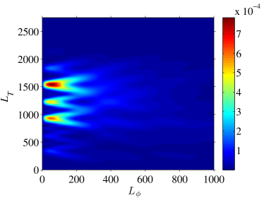
Figure 13: Theoretical contribution from the primary type-B connected $4$-point function to the correlation of the unbinned power spectra of the lens reconstruction and the (lensed) temperature power spectrum. The covariance (102) is converted to a correlation using the same conversion factor as in Eq. (37). Correlations for $L_{\phi}>1000$ are too small to be visible in this plot.

The correlation of unbinned power spectra from the primary term of Eq. (102) is shown in Fig. 13. It is at most $0.08\%$, which is almost a factor of two larger than the maximum of the matter cosmic variance contribution [Eq. (111)] shown in Fig. 5a. The structure is very similar to that of the disconnected (noise) contribution [Eq. (35)] shown in Fig. 4a, but with the additional signal-to-noise factor of $C_{L}^{\phi\phi}/A_{L}$ that falls off rapidly for $L>200$. (Recall, $A_{L}=N_{L}^{(0)}$ for our choice of optimal weights.) Therefore the contribution of the primary type-B covariance to correlations between the lensing amplitudes $\hat{A}$ and $\hat{A}^{\prime}$ is suppressed compared to that of the disconnected noise contribution, reaching at most $2\%$ (see Fig. 8). It is also suppressed compared to the matter cosmic variance contribution because $\hat{A}^{\prime}$ gives most weight to CMB modes at the acoustic peaks and troughs where the primary type-B power correlation is small.

While the measured correlation of $\hat{A}$ and $\hat{A}^{\prime}$ is consistent with our theoretical expectations, the measurements are too noisy to test sub-dominant terms such as that in Eq. (102). In Fig. 4c, the lowest $L_{\phi}$ pixels show hints of the structure plotted in Fig. 13, but the measurements are, again, too noisy to provide a conclusive test of Eq. (102). The simulations do however imply that there cannot be significantly larger covariance contributions than the ones we model analytically.

Although the summation in the expression (103) for the non-primary type-B terms is restricted by triangle inequalities, its evaluation is still numerically challenging. We could only evaluate Eq. (103) for $30$ $(L,L^{\prime})$ pairs at $L\lesssim 400$, which is relevant for the current Planck lensing likelihood Planck Collaboration et al. (2013a). At these points the power correlation from Eq. (103) is at most around $4\times 10^{-5}$, which is an order of magnitude smaller than the maximum correlation from the primary term [Eq. (102)]. The structure of the correlation matrix seems similar to that of the primary term in the $L_{T}$ direction, but seems to peak towards higher $L_{\phi}$ (but we cannot assess the structure reliably from the small number of evaluation points). Moreover, given that our simulations do not show any significant excess covariance we expect the non-primary term of Eq. (103) to be negligible.

Appendix E Temperature-lensing power covariance from the connected CMB 6-point function

The $\mathcal{O}(\phi^{2})$ contribution to the connected part of the lensed temperature $6$-point function vanishes Kesden et al. (2002). Here we will compute the $\mathcal{O}(\phi^{4})$ terms. There are five types of terms, which involve $\delta^{4}T$, $\delta^{3}T\delta T$, $\delta^{2}T\delta^{2}T$, $\delta^{2}T\delta T\delta T$ or $\delta T\delta T\delta T\delta T$ with the appropriate number of factors of the unlensed CMB. Only the last two types of terms contribute to the connected 6-point function; the remaining terms contribute to the full six-point function but are cancelled when the connected 4-point and fully disconnected parts are removed.

Writing out only the two relevant types of terms, the full $6$-point function at $\mathcal{O}(\phi^{4})$ is ($\tilde{T}_{i}\equiv\tilde{T}_{l_{i}m_{i}}$)

$$\langle\tilde{T}_{1}\tilde{T}_{2}\tilde{T}_{3}\tilde{T}_{4}\tilde{T}_{5}\tilde{T}_{6}\rangle^{(4)}=\frac{1}{12}\left[\langle\delta^{2}T_{1}\delta T_{2}\delta T_{3}T_{4}T_{5}T_{6}\rangle+\mbox{all perms}\right]+\frac{1}{48}\left[\langle\delta T_{1}\delta T_{2}\delta T_{3}\delta T_{4}T_{5}T_{6}\rangle+\mbox{all perms}\right].$$ (104)

From this we must subtract the following terms involving the connected 4-point function,

$$\tfrac{1}{48}\big{[}\langle\tilde{T}_{1}\tilde{T}_{2}\tilde{T}_{3}\tilde{T}_{4}\rangle_{c}\langle\tilde{T}_{5}\tilde{T}_{6}\rangle+\mbox{all perms}\big{]} =\frac{1}{48}\big{[} 6\langle\delta T_{1}\delta T_{2}T_{3}T_{4}\rangle\langle\delta T_{5}\delta T_{6}\rangle+12\langle\delta T_{1}\delta T_{2}T_{3}T_{4}\rangle\langle\delta^{2}T_{5}T_{6}\rangle$$ (105)

$$+12\langle\delta^{2}T_{1}\delta T_{2}\delta T_{3}T_{4}\rangle\langle T_{5}T_{6}\rangle+\langle\delta T_{1}\delta T_{2}\delta T_{3}\delta T_{4}\rangle\langle T_{5}T_{6}\rangle$$

$$-\left(9\langle\delta T_{1}\delta T_{2}\rangle+24\langle\delta^{2}T_{1}T_{2}\rangle\right)\langle\delta T_{3}\delta T_{4}\rangle\langle T_{5}T_{6}\rangle+\mbox{all perms}\big{]}+\cdots,$$

and the fully disconnected part,

$$\langle\tilde{T}_{1}\tilde{T}_{2}\tilde{T}_{3}\tilde{T}_{4}\tilde{T}_{5}\tilde{T}_{6}\rangle^{(4)}_{\mathrm{disc}} = \tfrac{1}{2}\left[\langle\delta^{2}T_{1}\delta T_{2}\rangle\langle\delta T_{3}T_{4}\rangle\langle T_{5}T_{6}\rangle+\mbox{all perms}\right]+\tfrac{1}{4}\left[\langle\delta^{2}T_{1}T_{2}\rangle\langle\delta T_{3}\delta T_{4}\rangle\langle T_{5}T_{6}\rangle+\mbox{all perms}\right]$$ (106)

$$+\tfrac{1}{2}\left[\langle\delta^{2}T_{1}T_{2}\rangle\langle\delta T_{3}T_{4}\rangle\langle\delta T_{5}T_{6}\rangle+\mbox{all perms}\right]+\tfrac{1}{16}\left[\langle\delta T_{1}\delta T_{2}\rangle\langle\delta T_{3}\delta T_{4}\rangle\langle T_{5}T_{6}\rangle+\mbox{all perms}\right]$$

$$+\tfrac{1}{4}\left[\langle\delta T_{1}\delta T_{2}\rangle\langle\delta T_{3}T_{4}\rangle\langle\delta T_{5}T_{6}\rangle+\mbox{all perms}\right]+\cdots.$$

To evaluate these expressions, we use, for example,

$$\langle\delta T_{1}\delta T_{2}T_{3}T_{4}\rangle=\langle\delta T_{1}\delta T_{2}\rangle\langle T_{3}T_{4}\rangle+\langle\langle\delta T_{1}T_{3}\rangle_{\mathrm{CMB}}\langle\delta T_{2}T_{4}\rangle_{\mathrm{CMB}}\rangle_{\mathrm{LSS}}+\langle\langle\delta T_{1}T_{4}\rangle_{\mathrm{CMB}}\langle\delta T_{2}T_{3}\rangle_{\mathrm{CMB}}\rangle_{\mathrm{LSS}},$$ (107)

where $\langle\rangle_{\mathrm{CMB}}$ denotes averaging over unlensed CMB realisations and $\langle\rangle_{\mathrm{LSS}}$ denotes averaging over realisations of the lensing potential $\phi$. Rewriting the other $4$- and $6$-point functions in a similar way gives the following final expression for the connected 6-point function:

$$\langle\tilde{T}_{1}\tilde{T}_{2}\tilde{T}_{3}\tilde{T}_{4}\tilde{T}_{5}\tilde{T}_{6}\rangle^{(4)}_{c} = \tfrac{1}{2}\mathrm{cov}_{\mathrm{LSS}}\left(\langle\delta^{2}T_{1}T_{2}\rangle_{\mathrm{CMB}},\langle\delta T_{3}T_{4}\rangle_{\mathrm{CMB}}\langle\delta T_{5}T_{6}\rangle_{\mathrm{CMB}}\right)+\mbox{all perms}$$ (108)

$$+\tfrac{1}{4}\mathrm{cov}_{\mathrm{LSS}}\left(\langle\delta T_{1}\delta T_{2}\rangle_{\mathrm{CMB}},\langle\delta T_{3}T_{4}\rangle_{\mathrm{CMB}}\langle\delta T_{5}T_{6}\rangle_{\mathrm{CMB}}\right)+\mbox{all perms}$$

$$= \tfrac{1}{16}\mathrm{cov}_{\mathrm{LSS}}\left(\langle\tilde{T}_{1}\tilde{T}_{2}\rangle^{(2)}_{\mathrm{CMB}},\langle\tilde{T}_{3}\tilde{T}_{4}\rangle^{(1)}_{\mathrm{CMB}}\langle\tilde{T}_{5}\tilde{T}_{6}\rangle^{(1)}_{\mathrm{CMB}}\right)+\mbox{all perms}.$$

The result is written in terms of the covariance over different realisations of the lensing potential, $\mathrm{cov}_{\mathrm{LSS}}(X,Y)\equiv\langle XY\rangle_{\mathrm{LSS}}-\langle X\rangle_{\mathrm{LSS}}\langle Y\rangle_{\mathrm{LSS}}$.

We expect only a few of the $720$ permutations in Eq. (108) to be relevant for the lensing-temperature power covariance [Eq. (33)]. The weights $\tilde{g}$ in Eq. (33) impose triangle conditions on $l_{1},l_{2},L$ and $l_{3},l_{4},L$, which constrain the summation volume (especially at low $L$ where the lensing power dominates). Terms that couple e.g. $\langle\tilde{T}_{1}\tilde{T}_{3}\rangle_{\text{CMB}}$ impose an additional triangle constraint on $l_{1},l_{3}$ and a lensing multipole $\tilde{L}$, which reduces the summation volume further. This is not the case for couplings of the type $\langle\tilde{T}_{1}\tilde{T}_{2}\rangle_{\text{CMB}}$ and $\langle\tilde{T}_{3}\tilde{T}_{4}\rangle_{\text{CMB}}$. For this reason we expect the dominant terms to come from the couplings $12$, $34$ and $(L^{\prime},M^{\prime};L^{\prime},-M^{\prime})$ in (33), i.e. terms which factor most under the weights Hanson et al. (2011). The dominant contribution of the connected $6$-point function at $\mathcal{O}(\phi^{4})$ to the lensing-temperature power covariance is therefore expected to come from

$$(-1)^{M^{\prime}}\langle\tilde{T}_{1}\tilde{T}_{2}\tilde{T}_{3}\tilde{T}_{4}\tilde{T}_{L^{\prime}M^{\prime}}\tilde{T}_{L^{\prime},-M^{\prime}}\rangle_{c,\mathrm{dom.}}^{(4)} = \mathrm{cov}_{\mathrm{LSS}}\left(\langle\tilde{T}_{L^{\prime}M^{\prime}}\tilde{T}^{*}_{L^{\prime}M^{\prime}}\rangle^{(2)}_{\mathrm{CMB}},\langle\tilde{T}_{1}\tilde{T}_{2}\rangle^{(1)}_{\mathrm{CMB}}\langle\tilde{T}_{3}\tilde{T}_{4}\rangle^{(1)}_{\mathrm{CMB}}\right)$$ (109)

$$+2\,\mathrm{cov}_{\mathrm{LSS}}\left(\langle\tilde{T}_{1}\tilde{T}_{2}\rangle_{\mathrm{CMB}}^{(2)},\langle\tilde{T}_{L^{\prime}M^{\prime}}\tilde{T}^{*}_{L^{\prime}M^{\prime}}\rangle^{(1)}_{\mathrm{CMB}}\langle\tilde{T}_{3}\tilde{T}_{4}\rangle^{(1)}_{\mathrm{CMB}}\right).$$

Here, we have used the result that permutations of the form $1\leftrightarrow 2$, $3\leftrightarrow 4$, $(12)\leftrightarrow(34)$ and $(L^{\prime},M^{\prime})\leftrightarrow(L^{\prime},-M^{\prime})$ all lead to the same contribution to Eq. (33).

The $\langle\tilde{T}_{1}\tilde{T}_{2}\rangle^{(1)}_{\text{CMB}}$ term on the right of Eq. (109) evaluates to

$$\langle\tilde{T}_{1}\tilde{T}_{2}\rangle^{(1)}_{\mathrm{CMB}} = \sum_{L_{1}M_{1}}(-1)^{M_{1}}\left(\begin{matrix}l_{1}&l_{2}&L_{1}\\ m_{1}&m_{2}&-M_{1}\end{matrix}\right)f_{l_{1}L_{1}l_{2}}\phi_{L_{1}M_{1}},$$ (110)

which combines with the weights, normalisation and one of the $3j$ symbols in Eq. (33) to give $\phi_{LM}+\mathcal{O}(\phi^{2})$. Similarly, the $\langle\tilde{T}_{3}\tilde{T}_{4}\rangle^{(1)}_{\text{CMB}}$ term returns $\phi_{L,-M}$. Equation (110) also shows that the second term on the right of Eq. (109) does not contribute to the power covariance since $\langle\tilde{T}_{L^{\prime}M^{\prime}}\tilde{T}^{*}_{L^{\prime}M^{\prime}}\rangle^{(1)}_{\text{CMB}}$ returns the monopole of $\phi$ on summing over $M^{\prime}$.

Putting these pieces together, and using Eq. (44), finally gives

$$\mathrm{cov}(\hat{C}^{\hat{\phi}\hat{\phi}}_{L},\hat{C}^{\tilde{T}\tilde{T}}_{L^{\prime}})_{\langle\tilde{T}_{1}\cdots\tilde{T}_{6}\rangle_{c,\mathrm{dom.}}^{(4)}} = \sum_{L^{\prime\prime}}\frac{\partial C^{\tilde{T}\tilde{T}}_{L^{\prime}}}{\partial C^{\phi\phi}_{L^{\prime\prime}}}\text{cov}_{\text{LSS}}(\hat{C}^{\phi\phi}_{L^{\prime\prime}},\hat{C}_{L}^{\phi\phi})+\mathcal{O}(\phi^{5})$$ (111)

$$= \frac{2}{2L+1}(C^{\phi\phi}_{L})^{2}\frac{\partial C^{\tilde{T}\tilde{T}}_{L^{\prime}}}{\partial C^{\phi\phi}_{L}}+\mathcal{O}(\phi^{5}).$$

Appendix F Effect of $C^{T\phi}$

In this appendix we discuss the contribution of the ISW-induced large-scale $C^{T\phi}$ correlation on the temperature-lensing power covariance. We first compute corrections due to the ISW-lensing bispectrum and then the ones due to corrections of the lensed temperature power spectrum.

The lensed temperature $6$-point function in the temperature-lensing power covariance of Eq. (33) involves the following 3-point terms:

$$\langle\tilde{T}_{\underline{l}_{1}}\tilde{T}_{\underline{l}_{2}}\tilde{T}_{\underline{l}_{3}}\tilde{T}_{\underline{l}_{4}}\tilde{T}_{L^{\prime}M^{\prime}}\tilde{T}_{L^{\prime}\,-M^{\prime}}\rangle|_{\text{3-pt},C^{T\phi}}=\langle\tilde{T}_{\underline{l}_{1}}\tilde{T}_{\underline{l}_{2}}\tilde{T}_{\underline{l}_{3}}\rangle^{\mathrm{ISW}}\langle\tilde{T}_{\underline{l}_{4}}\tilde{T}_{L^{\prime}M^{\prime}}\tilde{T}_{L^{\prime}\,-M^{\prime}}\rangle^{\mathrm{ISW}}+9\,\mathrm{perms},$$ (112)

where the non-perturbative ISW-lensing bispectrum is approximately given by Lewis et al. (2011); Hanson et al. (2009b)

$$\langle\tilde{T}_{\underline{l}_{1}}\tilde{T}_{\underline{l}_{2}}\tilde{T}_{\underline{l}_{3}}\rangle^{\mathrm{ISW}}=\left(\begin{matrix}l_{1}&l_{2}&l_{3}\\ m_{1}&m_{2}&m_{3}\end{matrix}\right)B^{\mathrm{ISW}}_{l_{1}l_{2}l_{3}}=\left(\begin{matrix}l_{1}&l_{2}&l_{3}\\ m_{1}&m_{2}&m_{3}\end{matrix}\right)C^{T\phi}_{l_{1}}\tilde{f}_{l_{2}l_{1}l_{3}}+2\,\mbox{perms}.$$ (113)

While the contribution to Eq. (33) from the coupling $(123)(4L^{\prime}L^{\prime})$, which is written out explicitly in Eq. (112), vanishes on summing over $M^{\prime}$, the couplings of type $(12L^{\prime})(34L^{\prime})$ yield the diagonal covariance contribution

$$\mathrm{cov}(\hat{C}^{\hat{\phi}\hat{\phi}}_{L},\hat{C}^{\tilde{T}\tilde{T}}_{L^{\prime},\mathrm{expt}})|_{\text{3-pt.},C^{T\phi}}^{(12L^{\prime}),(34L^{\prime})}=\delta_{LL^{\prime}}\frac{2A_{L}^{2}}{(2L+1)^{3}}\left[\sum_{l_{1}l_{2}}\tilde{g}_{l_{1}l_{2}}(L)B^{\mathrm{ISW}}_{l_{1}l_{2}L}\right]^{2}\approx\delta_{LL^{\prime}}\frac{2}{2L+1}(C^{T\phi}_{L})^{2}.$$ (114)

The approximation on the right is simply the covariance between the power spectra of the input lensing potential and the lensed temperature, an intuitive result that we might have anticipated. For our Planck-like parameters, the corresponding power correlation is always less than $5\%$ and rapidly decreases with increasing multipoles, being less than $0.1\%$ for $L\geq 60$ (see Fig. 14). The induced correlation of the lensing amplitudes $A$ and $A^{\prime}$ is less than $10^{-5}$ and therefore negligible. This small correlation arises because most of the information on the lensing amplitude from the temperature power spectrum comes from small scales. The power correlation due to the ISW-lensing effect is small on these scales, and, additionally, there is limited information in the lensing reconstruction on such scales as the signal-to-noise is very low there. We expect that couplings of the type $(13L^{\prime})(24L^{\prime})$ in Eq. (112), that do not factor under the weights, are further suppressed as they limit the summation volume.

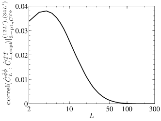
Figure 14: ISW-lensing bispectrum contribution of Eq. (114) to the diagonal unbinned temperature-lensing power correlation. The difference between the full expression and the approximation in Eq. (114) is too small to be visible in this plot.

The ISW-induced change in the lensed temperature power spectrum,

$$\Delta C^{\tilde{T}\tilde{T}}_{L}=C^{\tilde{T}\tilde{T}}_{L}-C^{\tilde{T}\tilde{T}}_{L}|_{C^{T\phi}=0}=\frac{1}{2L+1}\sum\limits_{L_{1},L_{2}}F^{2}_{LL_{1}L_{2}}C_{L_{1}}^{T\phi}C_{L_{2}}^{T\phi},$$ (115)

leads to a correction of the disconnected noise contribution [Eq. (35)] to the temperature-lensing power covariance which is also second order in $C^{T\phi}$. The correction has a similar structure to the noise contribution itself (shown in Fig. 4a), but it is around $10^{6}$ times smaller and induces a lensing amplitude correlation of $\mathcal{O}(10^{-9})$ that is totally negligible.

References

• Lewis and Challinor (2006) A. Lewis and A. Challinor, Physics Reports 429, 1 (2006), arXiv:astro-ph/0601594.
• Zaldarriaga and Seljak (1999) M. Zaldarriaga and U. Seljak, Phys. Rev. D 59, 123507 (1999), arXiv:astro-ph/9810257.
• Hu (2001a) W. Hu, APJL  557, L79 (2001a), arXiv:astro-ph/0105424.
• Hu (2002) W. Hu, Phys. Rev. D 65, 023003 (2002), arXiv:astro-ph/0108090.
• Kaplinghat et al. (2003) M. Kaplinghat, L. Knox, and Y.-S. Song, Physical Review Letters 91, 241301 (2003), arXiv:astro-ph/0303344.
• Verde and Spergel (2002) L. Verde and D. N. Spergel, Phys. Rev. D 65, 043007 (2002), arXiv:astro-ph/0108179.
• Acquaviva et al. (2004) V. Acquaviva, C. Baccigalupi, and F. Perrotta, Phys. Rev. D 70, 023515 (2004), arXiv:astro-ph/0403654.
• Calabrese et al. (2008) E. Calabrese, A. Slosar, A. Melchiorri, G. F. Smoot, and O. Zahn, Phys. Rev. D 77, 123531 (2008), 0803.2309.
• Hall and Challinor (2012) A. C. Hall and A. Challinor, Mon. Not. R. Astron. Soc. 425, 1170 (2012), 1205.6172.
• Das et al. (2011) S. Das, B. D. Sherwin, P. Aguirre, J. W. Appel, J. R. Bond, C. S. Carvalho, M. J. Devlin, J. Dunkley, R. Dünner, T. Essinger-Hileman, et al., Physical Review Letters 107, 021301 (2011), 1103.2124.
• Das et al. (2013) S. Das, T. Louis, M. R. Nolta, G. E. Addison, E. S. Battistelli, J. Bond, E. Calabrese, D. C. M. J. Devlin, S. Dicker, J. Dunkley, et al., ArXiv e-prints (2013), 1301.1037.
• van Engelen et al. (2012) A. van Engelen, R. Keisler, O. Zahn, K. A. Aird, B. A. Benson, L. E. Bleem, J. E. Carlstrom, C. L. Chang, H. M. Cho, T. M. Crawford, et al., Astrophys. J.  756, 142 (2012), 1202.0546.
• Planck Collaboration et al. (2013a) Planck Collaboration, P. A. R. Ade, N. Aghanim, C. Armitage-Caplan, M. Arnaud, M. Ashdown, F. Atrio-Barandela, J. Aumont, C. Baccigalupi, A. J. Banday, et al., ArXiv e-prints (2013a), 1303.5077.
• Hu (2001b) W. Hu, Phys. Rev. D 64, 083005 (2001b), arXiv:astro-ph/0105117.
• Seljak (1996) U. Seljak, Astrophys. J.  463, 1 (1996), arXiv:astro-ph/9505109.
• Story et al. (2012) K. T. Story, C. L. Reichardt, Z. Hou, R. Keisler, K. A. Aird, B. A. Benson, L. E. Bleem, J. E. Carlstrom, C. L. Chang, H. Cho, et al., ArXiv e-prints (2012), 1210.7231.
• Planck Collaboration et al. (2013b) Planck Collaboration, P. A. R. Ade, N. Aghanim, C. Armitage-Caplan, M. Arnaud, M. Ashdown, F. Atrio-Barandela, J. Aumont, C. Baccigalupi, A. J. Banday, et al., ArXiv e-prints (2013b), 1303.5076.
• Hirata and Seljak (2003) C. M. Hirata and U. Seljak, Phys. Rev. D 67, 043001 (2003), arXiv:astro-ph/0209489.
• Sherwin et al. (2011) B. D. Sherwin, J. Dunkley, S. Das, J. W. Appel, J. R. Bond, C. S. Carvalho, M. J. Devlin, R. Dünner, T. Essinger-Hileman, J. W. Fowler, et al., Physical Review Letters 107, 021302 (2011), 1105.0419.
• Lesgourgues et al. (2006) J. Lesgourgues, L. Perotto, S. Pastor, and M. Piat, Phys. Rev. D 73, 045021 (2006), arXiv:astro-ph/0511735.
• Goldberg and Spergel (1999) D. M. Goldberg and D. N. Spergel, Phys. Rev. D 59, 103002 (1999), arXiv:astro-ph/9811251.
• Bond et al. (2000) J. R. Bond, A. H. Jaffe, and L. Knox, Astrophys. J.  533, 19 (2000), arXiv:astro-ph/9808264.
• Verde et al. (2003) L. Verde, H. V. Peiris, D. N. Spergel, M. R. Nolta, C. L. Bennett, M. Halpern, G. Hinshaw, N. Jarosik, A. Kogut, M. Limon, et al., Astrophys. J. Supp. 148, 195 (2003), arXiv:astro-ph/0302218.
• Smith et al. (2006a) S. Smith, A. Challinor, and G. Rocha, Phys. Rev. D 73, 023517 (2006a), arXiv:astro-ph/0511703.
• Hamimeche and Lewis (2008) S. Hamimeche and A. Lewis, Phys. Rev. D 77, 103013 (2008), 0801.0554.
• Hanson et al. (2011) D. Hanson, A. Challinor, G. Efstathiou, and P. Bielewicz, Phys. Rev. D 83, 043005 (2011), 1008.4403.
• Challinor and Chon (2002) A. Challinor and G. Chon, Phys. Rev. D 66, 127301 (2002), arXiv:astro-ph/0301064.
• Hu (2000) W. Hu, Phys. Rev. D 62, 043007 (2000), arXiv:astro-ph/0001303.
• Hu and Okamoto (2002) W. Hu and T. Okamoto, Astrophys. J.  574, 566 (2002), arXiv:astro-ph/0111606.
• Lewis et al. (2011) A. Lewis, A. Challinor, and D. Hanson, JCAP 3, 018 (2011), 1101.2234.
• Okamoto and Hu (2003) T. Okamoto and W. Hu, Phys. Rev. D 67, 083002 (2003), arXiv:astro-ph/0301031.
• Kesden et al. (2003) M. Kesden, A. Cooray, and M. Kamionkowski, Phys. Rev. D 67, 123507 (2003), arXiv:astro-ph/0302536.
• Namikawa et al. (2013) T. Namikawa, D. Hanson, and R. Takahashi, Mon. Not. R. Astron. Soc. 431, 609 (2013), 1209.0091.
• Regan et al. (2010) D. M. Regan, E. P. S. Shellard, and J. R. Fergusson, Phys. Rev. D 82, 023520 (2010), 1004.2915.
• NASA (2012) NASA, Lambda (2012), URL http://lambda.gsfc.nasa.gov/.
• Lewis (2005) A. Lewis, Phys. Rev. D 71, 083008 (2005), arXiv:astro-ph/0502469.
• Górski et al. (2005) K. M. Górski, E. Hivon, A. J. Banday, B. D. Wandelt, F. K. Hansen, M. Reinecke, and M. Bartelmann, Astrophys. J.  622, 759 (2005), arXiv:astro-ph/0409513.
• Smith et al. (2006b) K. M. Smith, W. Hu, and M. Kaplinghat, Phys. Rev. D 74, 123002 (2006b), arXiv:astro-ph/0607315.
• Li et al. (2007) C. Li, T. L. Smith, and A. Cooray, Phys. Rev. D 75, 083501 (2007), arXiv:astro-ph/0607494.
• Benoit-Lévy et al. (2012) A. Benoit-Lévy, K. M. Smith, and W. Hu, Phys. Rev. D 86, 123008 (2012), 1205.0474.
• Lewis et al. (2000) A. Lewis, A. Challinor, and A. Lasenby, Astrophys. J.  538, 473 (2000), arXiv:astro-ph/9911177.
• Challinor and Lewis (2005) A. Challinor and A. Lewis, Phys. Rev. D 71, 103010 (2005), arXiv:astro-ph/0502425.
• Kesden et al. (2002) M. Kesden, A. Cooray, and M. Kamionkowski, Phys. Rev. D 66, 083007 (2002), arXiv:astro-ph/0208325.
• Zahn et al. (2013) O. Zahn et al., in prep. (2013).
• Bucher et al. (2012) M. Bucher, C. S. Carvalho, K. Moodley, and M. Remazeilles, Phys. Rev. D 85, 043016 (2012), 1004.3285.
• Hanson et al. (2009a) D. Hanson, G. Rocha, and K. Górski, Mon. Not. R. Astron. Soc. 400, 2169 (2009a), 0907.1927.
• Sherwin and Das (2010) B. D. Sherwin and S. Das, ArXiv e-prints (2010), 1011.4510.
• (48) NIST Digital Library of Mathematical Functions, http://dlmf.nist.gov/, Release 1.0.5 of 2012-10-01, online companion to Olver et al. (2010), URL http://dlmf.nist.gov/.
• Hanson et al. (2009b) D. Hanson, K. M. Smith, A. Challinor, and M. Liguori, Phys. Rev. D 80, 083004 (2009b), 0905.4732.
• Olver et al. (2010) F. W. J. Olver, D. W. Lozier, R. F. Boisvert, and C. W. Clark, eds., NIST Handbook of Mathematical Functions (Cambridge University Press, New York, NY, 2010), print companion to NIS .