Text Compression using Abstract Numeration System on a Regular Language

Abstract

An abstract numeration system (ANS) is a numeration system that provides a one-to-one correspondence between the natural numbers and a regular language. In this paper, we define an ANS-based compression as an extension of this correspondence. In addition, we show the following results: 1) an average compression ratio is computable from a language, 2) an ANS-based compression runs in sublinear time with respect to the length of the input string, and 3) an ANS-based compression can be extended to block-based compression using a factorial language.

1 Introduction

Compression has been closely studied in the past and remains an important issue in the real world today. String compression methods that focus on the input distribution, such as entropy-based compression, have been thoroughly investigated. Grammar-based compressions have also been investigated. This latter method has been formalized as the smallest grammar problem, which constructs a minimal context-free grammar that can generate a given string [1].

Whereas these are the two major approaches to compression, an alternative approach uses the “ordering” of a given string in the given language, namely its ranking. Goldberg and Sipser define ranking-based compression and show that ranking in a context-free grammar is computable in polynomial time [2]. A summary of the ranking-based compression approach is available in the literature [3]. In another approach to ranking, a one-to-one correspondence between the natural numbers and a regular language, namely an abstract numeration system (ANS), has been proposed independently by Lecomte and Rigo [4]. The mathematical properties and abilities of an ANS were studied in [5].

The present paper presents an ANS-based compression on a regular language that uses base conversion between two regular languages, and lays the foundations of this approach. There are three main results from our research. First, we analyze the complexity of the algorithm for an ANS (see Table 1, §3). Second, we can find the average compression ratio of an ANS-based compression (see Theorem 4.1, §4.2). Third, we propose a block-based compression method that does not reduce the compression ratio by using a factorial language (see Theorem 5.1, §5).

2 Preliminaries

We first introduce some preliminary notions, notation, and theorems from the literature [6, 7, 5].

2.1 Regular languages and automata

The set of nonnegative integers is denoted by $\mathbb{N}\ni 0$, and the set of positive real numbers is denoted by $\mathbb{R^{+}}$. Let $A$ denote a finite set of symbols, with $A^{n}$ denoting the set of all strings of length $n$ over $A$. Let $A^{*}$ represent the set of all strings over $A$: $A^{*}:=\bigcup_{i=0}^{\infty}A^{i}.$ The string of length 0 is $\varepsilon$ ($A^{0}=\{\varepsilon\}$). A subset $L$ of $A^{*}$ is called a language over $A$. The characters $w$ and $\sigma$ are used to denote a string $w\in A^{*}$ and a symbol $\sigma\in A$. In addition, $|w|$ denotes the length of $w$ and $w_{i}$, such that $1\leq i\leq|w|$ denotes the $i$-th symbol of $w$. The power set of a set $S$ is written $\mathfrak{P}(S)$. A finite automaton ${\cal A}$ is a 5-tuple ${\cal A}=(Q,A,\delta,I,F)$, comprising a finite set of states $Q$, a finite set of input symbols $A$, a transition function $\delta:Q\times A\rightarrow\mathfrak{P}(Q)$, and a set of start and accepting states $I\subseteq Q$ and $F\subseteq Q$. The symbol like $|{\cal A}|$ denotes the number of states for the finite automaton ${\cal A}$. The set of all acceptable strings of ${\cal A}$ is denoted by $L({\cal A})$.

Definition 1 ([6])

An automaton ${\cal A}=(Q,A,\delta,I,F)$ is an unambiguous finite automaton (UFA) when it satisfies the following two conditions:

1. for every pair of states $(p,q)$ and every string $w$ in $A^{*}$, there exists at most one transition from $p$ to $q$ on input $w$ ($q\in\delta(p,w)$);

2. for every string $w$ in $L({\cal A})$, there exists a unique $p$ in $I$ and a unique $q$ in $F$ such that $q\in\delta(p,w)$. $\hfill\diamond$

Any deterministic finite automaton (DFA) will clearly satisfy the UFA conditions. To emphasize that an automaton is deterministic, we use ${\cal D}$ to denote a DFA. Similarly, we use ${\cal U}$ to denote a UFA, with ${\cal N}$ being used to denote a nondeterministic finite automaton (NFA). We will now focus on UFAs and DFAs. Although these classes are more limited than the NFA class, they are easy to handle, and are compatible with counting functions because of their unambiguity.

We introduce a matrix representation for an automaton. Because an automaton can be viewed as a digraph, its adjacency matrix can be derived naturally.

Definition 2 ([6])

The adjacency matrix $\bm{M}({\cal A})\in\mathbb{N}^{|{\cal A}|\times|{\cal A}|}$ of an automaton ${\cal A}$ is defined as $\bm{M}({\cal A})_{pq}:=\#\left\{\sigma\in A\mid q\in\delta(p,\sigma)\right\}$. The initial (row) vector $\bm{V}_{I}({\cal A})\in\mathbb{B}^{|{\cal A}|}$ and accepting (column) vector $\bm{V}_{F}({\cal A})^{T}\in\mathbb{B}^{|{\cal A}|}$ are defined as follows:

$$\bm{V}_{I}({\cal A})_{q}:=\text{if}\;q\in I\;\;\text{then}\;1\;\text{else}\;0,\;\;\;\;\;\;\bm{V}_{F}({\cal A})_{q} := \text{if}\;q\in F\;\text{then}\;1\;\text{else}\;0.$$

A triple $(\bm{M}({\cal A}),\bm{V}_{I}({\cal A}),\bm{V}_{F}({\cal A}))$ is called a matrix representation of ${\cal A}$. $\hfill\diamond$

In this paper, we will denote the set of eigenvalues of a matrix $\bm{M}$ by $\lambda(\bm{M})$, and denote the zero vector by $\bm{0}$.

2.2 Combinatorial complexity

In formal language theory, combinatorial complexity is formulated in terms of the complexity of the counting function $C_{L}$ of a language $L$ [7, 5, 8], which is defined as follows:   $C_{L}(n):=\#\left\{w\in L\mid|w|=n\right\}=\#(L\cap A^{n}),\;C_{L}^{\leq}(n):=\sum_{i=0}^{n}C_{L}(i)$. We note that a counting function $C_{L}$ can be calculated by using a trim UFA.

Lemma 1 ([5])

Consider a UFA ${\cal U}$ such that $L({\cal U})=L$. Then the following equation holds:

$$C_{L}(n)=\bm{V}_{I}\bm{M}^{n}\bm{V}_{F}.$$

Proof

The value $\bm{M}^{n}_{pq}$ of the adjacency matrix of the UFA ${\cal U}$ is exactly the number of paths of length $n$ from state $p$ to state $q$. Each value in vector $\bm{V}_{I}\bm{M}^{n}$ is therefore the number of paths of length $n$ from an initial state to one of the states. Consequently, the value obtained by multiplying the accepting vector by the vector $\bm{V}_{I}\bm{M}^{n}$, $\bm{V}_{I}\bm{M}^{n}\bm{V}_{F}$ is the number of acceptable paths of length $n$. Because ${\cal U}$ is unambiguous, there exists a one-to-one correspondence between paths and strings. ∎

Next, we introduce the important theorem about the asymptotic growth of a counting function for a regular language [9]. (This theorem will be needed in §4.2.) Here, we use the standard $\mathrm{O}$-, $\Omega$-, $\Theta$-notations, and the following more complicated definitions.

Definition 3 ([9])

The notation $f(n)=\bar{\Theta}(g(n))$ means that $f(n)=\mathrm{O}(g(n))$ and there exists a sequence $\{n_{i}\}_{1}^{\infty}$ and a constant $c>0$ such that $f(n_{i})\geq c\cdot g(n_{i})$ for all $i$. That is, the notation $\bar{\Theta}(g(n))$ is weaker than the notation $\Theta(g(n))$. $\hfill\diamond$

Definition 4 ([7])

Consider an automaton ${\cal A}$. The index of ${\cal A}$: $\mathrm{Ind}({\cal A})$ is defined as the maximum eigenvalue of the adjacency matrix of ${\cal A}$:

$$\mathrm{Ind}({\cal A}):=\max\{\alpha\in\lambda(\bm{M}({\cal A}))\}.$$

The polynomial index of ${\cal A}$: ${{\mathrm{Pd}}({\cal A})}$ is defined as the value obtained by subtracting 1 from the maximum number of strongly connected components (SCCs) of index $\mathrm{Ind}({\cal A})$ connected by a simple path in ${\cal A}$. $\hfill\diamond$

Theorem 2.1 (Shur [9])

Let a regular language $L$ be recognized by a trim DFA ${\cal D}$. Then, $C_{L}(n)=\bar{\Theta}(n^{{\mathrm{Pd}}({\cal D})}\mathrm{Ind}({\cal D})^{n})$ holds.

Remark 1

We omit the proof here, but note some known algorithmic results for graphs and matrices. Let $G$ be a digraph with $n$ vertices and $e$ paths. Then, SCC decomposition is computable in $\mathrm{O}(n+e)=\mathrm{O}(n^{2})$. The index of $G$ is approximately computable in $\mathrm{O}(n^{3})$ using the classical power method [10]. $\hfill\diamond$

Because the definitions of $\mathrm{Ind}({\cal D})$ and ${{\mathrm{Pd}}({\cal D})}$ are slightly complicated, it might be hard to grasp the meaning of Theorem 2.1. We therefore introduce the following simple examples of Lemma 1 and Theorem 2.1.

Figure 1: ${\cal D}_{fib}$ such that $L({\cal D}_{fib})=\{a,ba\}^{*}$

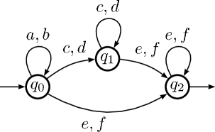
Figure 2: ${\cal D}_{poly}$ such that $L({\cal D}_{poly})=\{a,b\}^{*}\{c,d\}^{*}\{e,f\}^{+}$

Example 1

For the DFA ${\cal D}_{fib};\;L({\cal D}_{fib})=\{a,ba\}^{*}$, as shown in Figure 2, consider the counting function $C_{L}$. The matrix representation of ${\cal D}_{fib}$ is:

$$\bm{M}=\begin{pmatrix}1&1\\ 1&0\end{pmatrix},\;\;\;\;\bm{V}_{I}=\bm{V}_{F}^{T}=(1,0).$$

We can enumerate the sequence $C_{L}(n)$ up to five, as follows:

$$C_{L}(0) = \#\left\{\varepsilon\right\}=1,\;\;\;\;C_{L}(1)=\#\left\{a\right\}=1,\;\;\;\;C_{L}(2)=\#\left\{aa,ba\right\}=2,$$

$$C_{L}(3) = \#\left\{aaa,aba,baa\right\}=3,\;\;\;\;C_{L}(4)=\#\{aaaa,aaba,abaa,baaa,baba\}=5.$$

The adjacency matrix $\bm{M}$ is diagonalizable via a matrix $P$ because $\bm{M}$ has the set of eigenvalues $\lambda(\bm{M})=\left\{\alpha=\frac{1+\sqrt{5}}{2},\beta=\frac{1-\sqrt{5}}{2}\right\}$. Here, we obtain the following equation via Lemma 1:

$$C_{L}(n) = \bm{V}_{I}\bm{M}^{n}\bm{V}_{F}=\bm{V}_{I}\bm{PD}^{n}\bm{P}^{-1}\bm{V}_{F}=\frac{1}{\sqrt{5}}\bm{V}_{I}\begin{pmatrix}\alpha^{n+1}-\beta^{n+1}&\alpha^{n}-\beta^{n}\\[2.0pt] \alpha^{n}-\beta^{n}&\alpha^{n-1}-\beta^{n-1}\end{pmatrix}\bm{V}_{F}$$

$$= \frac{1}{\sqrt{5}}\left\{\left(\frac{1+\sqrt{5}}{2}\right)^{n+1}-\left(\frac{1-\sqrt{5}}{2}\right)^{n+1}\right\}.$$

From this, we find that $C_{L}(n)$ is the $(n+1)$-th Fibonacci number. $\hfill\diamond$

Example 2

The index of ${\cal D}_{fib}$ is $\frac{1+\sqrt{5}}{2}$. In addition, the polynomial index of ${\cal D}_{fib}$ is 0 because ${\cal D}_{fib}$ contains only one SCC, as does $\{q_{0}\}$. From Theorem 2.1, the following equation therefore holds. This matches the result of Example 1.

$$C_{L}(n)=\bar{\Theta}(n^{{\mathrm{Pd}}({\cal D}_{fib})}\mathrm{Ind}({\cal D}_{fib})^{n})=\bar{\Theta}\left(\left(\frac{1+\sqrt{5}}{2}\right)^{n}\right).$$

$\hfill\diamond$

Example 3

For the DFA ${\cal D}_{poly}$ such that $L({\cal D}_{poly})=\{a,b\}^{*}\{c,d\}^{*}\{e,f\}^{+}$, as shown in Figure 2, each state is a SCC and there are two self-loop transitions respectively. The index of ${\cal D}_{poly}$ is therefore $\mathrm{Ind}({\cal D}_{poly})=2$. Furthermore, the set of the SCCs that are connected by a simple path, except for each self-loop, are: $\{\{q_{0}\},\{q_{1}\}\},\;\;\{\{q_{1}\},\{q_{2}\}\},\;\;\{\{q_{0}\},\{q_{2}\}\},\;\;\{\{q_{0}\},\{q_{1}\},\{q_{2}\}\}.$ The polynomial index of the DFA ${\cal D}_{poly}$ is therefore ${{\mathrm{Pd}}({\cal D}_{poly})}=\#\{\{q_{0}\},\{q_{1}\},\{q_{2}\}\}-1=2$. Consequently, $C_{L}(n)=\bar{\Theta}(n^{2}2^{n})$ holds from Theorem 2.1.$\hfill\diamond$

Fact 1 ([9])

For any DFA ${\cal D}$ such that $L({\cal D})=L$, its index $\mathrm{Ind}({\cal D})$ is 0 or greater than or equal to 1 because the elements of adjacency matrices are positive integers. Moreover, there are only three possible patterns: 1) $\mathrm{Ind}({\cal D})=0\Leftrightarrow$ $L$ is a finite set, 2) $\mathrm{Ind}({\cal D})=1\Leftrightarrow$ $C_{L}(n)$ has polynomial growth, or 3) $\mathrm{Ind}({\cal D})>1\Leftrightarrow$ $C_{L}(n)$ has exponential growth. In addition, the index of ${\cal D}$ equals the maximum index of each SCC in ${\cal D}$.$\hfill\diamond$

Theorem 2.1 clarifies the asymptotic growth of the counting function. We now know that the index and polynomial index of a DFA ${\cal D}$ are not simply values, but are specific values of a regular language $L$ recognized by the DFA ${\cal D}$. For this reason, we introduce the following additional definition.

Definition 4 (addition)

Let a regular language $L$ be recognized by a DFA ${\cal D}$,

$$\mathrm{Ind}(L):=\mathrm{Ind}({\cal D}),\;\;\;\;{{\mathrm{Pd}}(L)}:=\mathrm{Ind}({\cal D}).$$

$\hfill\diamond$

2.3 Abstract numeration system

A numeration system is a system that represents a number as a string and vice versa, and is an area of mathematics in itself. Its representation abilities and the properties of algebraic operations on it have been widely studied [5, 4, 11]. An abstract numeration system has been proposed by Lecomte and Rigo in 1999 [4].

Definition 5 ([5])

Assume that $(A,<)$ is a totally ordered set of symbols. Then, the set $A^{*}$ is totally ordered by radix order $\prec$ defined as follows. Let $u,v$ be two strings in $A^{*}$. We write $u\prec v$ if either $|u|<|v|$ or $|u|=|v|$, and there exists $r,s,t\in A^{*},\;a,b\in A$ with $u=ras,v=rbt$ and $a<b$. By $u\preceq v$, we mean that either $u\prec v$ or $u=v$. The set $A^{*}$ can be totally ordered by lexicographic order. $\hfill\diamond$

Definition 6 ([5])

An ANS ${\cal S}$ is a triple $(L,A,<)$ comprising a totally ordered finite set of symbols $(A,<)$ and an infinite regular language $L$ over $(A,<)$. The order isomorphism map $\mathop{\mathrm{rep}}\nolimits_{\cal S}:\mathbb{N}\rightarrow L$ is the one-to-one correspondence mapping $n\in\mathbb{N}$ to the $(n+1)$-th string in the radix-ordered language $L$. The inverse map is denoted by $\mathop{\mathrm{val}}\nolimits_{\cal S}:L\rightarrow\mathbb{N}$. $\hfill\diamond$

An ANS is not only simple but also flexible. The following example shows that an ANS can represent ordinary $2$-ary (binary) or $10$-ary (decimal) systems.

Example 4

Consider the ANS ${\cal S}_{2}=(L,\{0,1\},<)$ such that $L=\{0\}\cup\{1\}\{0,1\}^{*},$
$0<1$. The strings in $L$ will be ordered by radix order as $\{0,1,10,11,100,\ldots\}$, with ${\cal S}_{2}$ generating the binary system in this manner. That is, the mapping:

$$\mathop{\mathrm{rep}}\nolimits_{{\cal S}_{2}}(0)=0,\;\mathop{\mathrm{rep}}\nolimits_{{\cal S}_{2}}(1)=1,\;\mathop{\mathrm{rep}}\nolimits_{{\cal S}_{2}}(2)=10,\mathop{\mathrm{rep}}\nolimits_{{\cal S}_{2}}(3)=11,\;\mathop{\mathrm{rep}}\nolimits_{{\cal S}_{2}}(4)=100,\;\ldots$$

$$\mathop{\mathrm{val}}\nolimits_{{\cal S}_{2}}(0)=0,\;\;\mathop{\mathrm{val}}\nolimits_{{\cal S}_{2}}(1)=1,\;\mathop{\mathrm{val}}\nolimits_{{\cal S}_{2}}(10)=2,\;\mathop{\mathrm{val}}\nolimits_{{\cal S}_{2}}(11)=3,\;\mathop{\mathrm{val}}\nolimits_{{\cal S}_{2}}(100)=4,\;\ldots$$

makes a correspondence between $\mathbb{N}$ and its binary representation. $\hfill\diamond$

In fact, in terms of recognizability, it is known that an ANS is more powerful than classical $k$-ary systems. More details about ANSs are available from the work of Lecomte and Rigo [5].

3 Algorithms for ANSs using matrices and vectors

In this section, we provide algorithms for $\mathop{\mathrm{rep}}\nolimits_{\cal S}$ and $\mathop{\mathrm{val}}\nolimits_{\cal S}$. The main mechanisms in these algorithms are sum and product operations on a trim DFA and its matrix representation. The concepts behind the algorithms in this section are described in the work of Lecomte and Rigo [5]. Here, we interpret these algorithms in terms of a matrix representation and analyze their complexity.

    Algorithm 1 $\mathop{\mathrm{val}}\nolimits_{\cal S}$  

0:  $w\in L$

0:  $n=\mathop{\mathrm{val}}\nolimits_{\cal S}(w)$

1:  $q\leftarrow q_{0}\in I$

2:  $\bm{V}\leftarrow\bm{0}\in\mathbb{N}^{|w|}$

3:  for $i=1\to|w|$ do

4:     $\bm{V}\leftarrow\bm{V}+\bm{V}_{q}^{w_{i}}+\bm{V}_{I}$

5:     $q\leftarrow\delta(q,w_{i})$

6:     if $i<|w|$ then

7:        $\bm{V}\leftarrow\bm{V}\bm{M}$

8:     end if

9:  end for

10:  $n\leftarrow\bm{V}\bm{V}_{F}$

 

    Algorithm 2 $\mathop{\mathrm{rep}}\nolimits_{\cal S}$ ([5], modified)  

0:  $0\leq n<\#L$

0:  $w=\mathop{\mathrm{rep}}\nolimits_{\cal S}(n)$

1:  $q\leftarrow q_{0}\in I$

2:  $\ell\leftarrow\max_{\ell}(C_{L}^{\leq}(\ell-1)\leq n)$

3:  $m\leftarrow n-C_{L}^{\leq}(\ell-1)$

4:  $w\leftarrow\varepsilon$

5:  for $i=\ell-1\to 0$ do

6:     $\sigma\leftarrow\displaystyle\min_{<}{A}$

7:     while $(\bm{M}^{i})_{\delta(q,\sigma)}\bm{V}_{F}\leq m$ do

8:        $m\leftarrow m-(\bm{M}^{i})_{\delta(q,\sigma)}\bm{V}_{F}$

9:        $\sigma\leftarrow\min\{\sigma^{\prime}\in A\mid\sigma<\sigma^{\prime}\}$

10:     end while

11:     $w\leftarrow w\sigma$

12:     $q\leftarrow\delta(q,\sigma)$

13:  end for

 

Table 1: The complexities of Algorithm 1 and Algorithm 2

	Time complexity	M–M	M–V	V–V
$\mathop{\mathrm{val}}\nolimits_{\cal S}(w)$	$\Theta(|w|\times\mathfrak{M}(|w|)\times|{\cal D}|^{2})$	$0$	$|w|-1$	1
$\mathop{\mathrm{rep}}\nolimits_{\cal S}(n)$	$\mathrm{O}(\ell\log\ell\times\mathfrak{M}(\ell\log\ell)\times\mathfrak{MM}(|{\cal D}|))$	$\mathrm{O}(\ell\log\ell)$	$0$	$\mathrm{O}(\ell\times|A|)$
Let $\ell=|\mathop{\mathrm{rep}}\nolimits_{\cal S}(n)|$. M–M, M–V, and V–V denote the number of matrix–matrix,
matrix–vector, and vector–vector multiplications, respectively.

We omit the details of Algorithm 1 ($\mathop{\mathrm{val}}\nolimits_{\cal S}$) and Algorithm 2 ($\mathop{\mathrm{rep}}\nolimits_{\cal S}$) for reasons of brevity. Table 1 shows the complexities of Algorithm 1 and Algorithm 2. The symbol $\mathfrak{M}(n)$ and $\mathfrak{MM}(n)$ denote the complexity of $n$-bit integer multiplication and the number of factor multiplications in the $n\times n$ matrix multiplication. The implementation of these algorithms has been published by the author .

Remark 2

In practice, there are efficient integer-multiplication algorithms such as the Schönhage–Strassen algorithm ($\mathfrak{M}(n)=\mathrm{O}(n\log n\log\log n)$) or the Fürer algorithm ($\mathfrak{M}(n)=2^{\mathrm{O}(\log^{*}{n})}$) [12]. The matrix multiplication in the algorithm for $\mathop{\mathrm{rep}}\nolimits_{\cal S}$ is the bottleneck. The Strassen algorithm ($\mathfrak{MM}(n)=\mathrm{O}(n^{2.807})$) is widely known and can be used as an efficient matrix-multiplication algorithm [10]. $\hfill\diamond$

4 ANSs and compression

In this section, we extend the notion of a one-to-one correspondence between $\mathbb{N}$ and a language to one between two regular languages, which involves a base conversion in ANSs. Moreover, we investigate its application to compression, especially its compression ratio.

4.1 Base conversion in ANSs

A base conversion ${\cal B}_{{\cal S}\rightarrow{\cal S}^{\prime}}:L\rightarrow L^{\prime}$ is an order isomorphism function between L and L’.

Definition 7

Consider two ANSs, ${\cal S}=(L,A,<)$ and ${\cal S}^{\prime}=(L^{\prime},A^{\prime},<^{\prime})$. A base conversion ${\cal B}_{{\cal S}\rightarrow{\cal S}^{\prime}}$ between ${\cal S}$ and ${\cal S}^{\prime}$ is defined as:

$$\mathop{\cal B}\limits_{{\cal S}\rightarrow{\cal S}^{\prime}}(w):=\mathop{\mathrm{rep}}\nolimits_{{\cal S}^{\prime}}(\mathop{\mathrm{val}}\nolimits_{\cal S}(w)).$$

$\hfill\diamond$

Remark 3

Consider two ANSs, ${\cal S}=(L,A,<)$ and ${\cal S}^{\prime}=(L^{\prime},A^{\prime},<^{\prime})$, and two DFAs, ${\cal D}$ and ${\cal D}^{\prime}$, such that $L=L({\cal D}),L^{\prime}=L({\cal D}^{\prime})$, and a string $w\in L$. For the number $\ell=|\mathop{\mathrm{rep}}\nolimits_{{\cal S}^{\prime}}(\mathop{\mathrm{val}}\nolimits_{\cal S}(w))|$, the complexity of a base conversion ${\cal B}_{{\cal S}\rightarrow{\cal S}^{\prime}}$ is as follows (see Table 1):

$$\Theta(|w|\times\mathfrak{M}(|w|)\times|{\cal D}|^{2})+\mathrm{O}(\ell\log\ell\times\mathfrak{M}(\ell\log\ell)\times\mathfrak{MM}(|{\cal D}^{\prime}|)).$$

$\hfill\diamond$

4.2 Compression ratio

In general, the compression ratio is defined as the ratio of the length of the input string to that of the output (compressed) string. This notion can be applied naturally to a base conversion in ANSs.

Definition 8

Consider two ANSs, ${\cal S}=(L,A,<)$ and ${\cal S}^{\prime}=(L^{\prime},A^{\prime},<^{\prime})$. The compression ratio $\mathrm{CR}$ of a base conversion ${\cal B}_{{\cal S}\rightarrow{\cal S}^{\prime}}$ is defined as follows.

• For a string $w\in L:\;\;\;\;\mathrm{CR}({\cal B}_{{\cal S}\rightarrow{\cal S}^{\prime}},w):=\left|{\cal B}_{{\cal S}\rightarrow{\cal S}^{\prime}}(w)\right|/\left|w\right|.$

• For a number $n\in\mathbb{N}:\;\;\mathrm{CR}({\cal B}_{{\cal S}\rightarrow{\cal S}^{\prime}},n):=\mathrm{CR}({\cal B}_{{\cal S}\rightarrow{\cal S}^{\prime}},\max_{\prec}(L\cap A^{n})).$
  Note that $\max_{\prec}(L\cap A^{n}$) is the maximum, under the radix order $\prec$, string that has the length $n$.

• For a regular language $L$, the limit of compression ratio is defined as:

  $$\mathrm{CR}({\cal B}_{{\cal S}\rightarrow{\cal S}^{\prime}}):=\displaystyle\lim_{|w\in L|\rightarrow\infty}\mathrm{CR}({\cal B}_{{\cal S}\rightarrow{\cal S}^{\prime}},w).$$

  We note that if the limit of compression ratio converges, then its limit value coincides with the average compression ratio of ${\cal B}_{{\cal S}\rightarrow{\cal S}^{\prime}}$:

  $$\lim_{|w\in L|\rightarrow\infty}\mathrm{CR}({\cal B}_{{\cal S}\rightarrow{\cal S}^{\prime}},w)=\displaystyle\lim_{n\rightarrow\infty}\frac{1}{n}\sum_{i=0}^{n}\mathrm{CR}({\cal B}_{{\cal S}\rightarrow{\cal S}^{\prime}},\mathop{\mathrm{rep}}\nolimits_{\cal S}(i)).$$

The base conversion ${\cal B}_{{\cal S}\rightarrow{\cal S}^{\prime}}$ is a “compression” if and only if $\mathrm{CR}({\cal B}_{{\cal S}\rightarrow{\cal S}^{\prime}})\leq 1$.$\hfill\diamond$

At the present time, it is not clear whether the limit of compression ratio of a base conversion $\mathrm{CR}({\cal B}_{{\cal S}\rightarrow{\cal S}^{\prime}})$ converges or diverges.

We now introduce Theorem 4.1 to clarify the limit value. This requires following Lemma 2 about counting functions.

Lemma 2

For any regular language $L$, the following equation holds:

$$C_{L}^{\leq}(n)=\begin{cases}\Theta(C_{L}(n))=\Theta(n^{{{\mathrm{Pd}}(L)}}\mathrm{Ind}(L)^{n})&\mathrm{if}\;\mathrm{Ind}(L)>1,\;\;\;\;\;\;\mathrm{(i)}\\ \Theta(n\times C_{L}(n))=\Theta(n^{{{\mathrm{Pd}}(L)}+1})&\mathrm{if}\;\mathrm{Ind}(L)=1.\;\;\;\;\;\;\mathrm{(ii)}\end{cases}$$

Proof

In case (i), the equation $C_{L}^{\leq}(n)=\bar{\Omega}(n^{{\mathrm{Pd}}(L)}\mathrm{Ind}(L)^{n})$ always holds because $C_{L}(n)\leq C_{L}^{\leq}(n)$ by definition. From the monotonicity of the function $C_{L}^{\leq}$, the following equations hold:

$$C_{L}^{\leq}(n) = \Omega(n^{{\mathrm{Pd}}(L)}\mathrm{Ind}(L)^{n}),$$ (1)

$$C_{L}^{\leq}(n) = \mathrm{O}\left(\sum_{i=0}^{n}i^{{\mathrm{Pd}}(L)}\mathrm{Ind}(L)^{i}\right)=\mathrm{O}\left(n^{{\mathrm{Pd}}(L)}\sum_{i=0}^{n}\mathrm{Ind}(L)^{i}\right)$$ (2)

$$= \mathrm{O}(n^{{\mathrm{Pd}}(L)}\mathrm{Ind}(L)^{n}).$$

From Equations (1) and (2), the upper and lower bounds are equal.

$$.\raisebox{4.30554pt}{.}.\;\;\;\;C_{L}^{\leq}(n)=\Theta(n^{{\mathrm{Pd}}(L)}\mathrm{Ind}(L)^{n}).$$

In case (ii), by Theorem 2.1, we can obtain the following equation:

$$C_{L}^{\leq}(n)=\bar{\Theta}\left(\sum_{i=0}^{n}i^{{\mathrm{Pd}}(L)}\mathrm{Ind}(L)^{i}\right)=\bar{\Theta}\left(\sum_{i=0}^{n}i^{{\mathrm{Pd}}(L)}\right)=\bar{\Theta}(n^{{{\mathrm{Pd}}(L)}+1}).$$ (3)

Note that the last transformation in Equation (3) uses a power sum formula. Clearly, $C_{L}^{\leq}(n)=\Omega(n^{{{\mathrm{Pd}}(L)}+1})$ holds from the monotonicity of the function $C_{L}^{\leq}$.

$$.\raisebox{4.30554pt}{.}.\;\;\;\;C_{L}^{\leq}(n)=\Theta(n^{{{\mathrm{Pd}}(L)}+1}).$$

$\hfill\diamond$

Theorem 4.1 (The compression ratio theorem)

Consider two ANSs, ${\cal S}=(L,A,<)$ and ${\cal S}^{\prime}=(L^{\prime},A^{\prime},<^{\prime})$. The average compression ratio of a base conversion ${\cal B}_{{\cal S}\rightarrow{\cal S}^{\prime}}:L\rightarrow L^{\prime}$ satisfies the following conditions:

1. If $\mathrm{Ind}(L^{\prime})>1$, then $\mathrm{CR}({\cal B}_{{\cal S}\rightarrow{\cal S}^{\prime}})=\log\mathrm{Ind}(L)/\log\mathrm{Ind}(L^{\prime})$,

2. If $\mathrm{Ind}(L)>\mathrm{Ind}(L^{\prime})=1$, then $\mathrm{CR}({\cal B}_{{\cal S}\rightarrow{\cal S}^{\prime}})=\infty$,

3. If $\mathrm{Ind}(L)=\mathrm{Ind}(L^{\prime})=1$, then:

   $$\mathrm{CR}({\cal B}_{{\cal S}\rightarrow{\cal S}^{\prime}})=\begin{cases}0&\text{if}\;\;\;{{\mathrm{Pd}}(L)}<{{\mathrm{Pd}}(L^{\prime})},\\ \text{in a finite interval}&\text{if}\;\;\;{{\mathrm{Pd}}(L)}={{\mathrm{Pd}}(L^{\prime})},\\ \infty&\text{if}\;\;\;{{\mathrm{Pd}}(L)}>{{\mathrm{Pd}}(L^{\prime})}.\end{cases}$$

Proof

Consider $w\in L$ and $w^{\prime}\in L^{\prime}$ such that $w^{\prime}={\cal B}_{{\cal S}\rightarrow{\cal S}^{\prime}}(w)$. That is, $\mathop{\mathrm{val}}\nolimits_{\cal S}(w)=\mathop{\mathrm{val}}\nolimits_{\cal S}^{\prime}(w)$. From Definition 8, the following equation holds:

$$\mathrm{CR}({\cal B}_{{\cal S}\rightarrow{\cal S}^{\prime}})=\displaystyle\lim_{|w\in L|\rightarrow\infty}\frac{\left|w^{\prime}\right|}{\left|w\right|}.$$

Moreover, in the case of $\lim_{|w\in L|\rightarrow\infty}$, for each value of $\mathop{\mathrm{val}}\nolimits_{{\cal S}}(w),\mathop{\mathrm{val}}\nolimits_{{\cal S}^{\prime}}(w^{\prime})$ and $|w^{\prime}|$ diverge to infinity. This is because the following inequalities:

$$C_{L}^{\leq}(|w|-1)\leq\mathop{\mathrm{val}}\nolimits_{{\cal S}}(w)<C_{L}^{\leq}(|w|),$$ (4)

$$C_{L}^{\prime\leq}(|w^{\prime}|-1)\leq\mathop{\mathrm{val}}\nolimits_{{\cal S}^{\prime}}(w^{\prime})<C_{L}^{\prime\leq}(|w^{\prime}|)$$ (5)

clearly always hold, from Definition 6. We can then give a proof for each of the conditions (i)–(iii) based on Inequalities (4) and (5) and the following Equation (6):

$$\mathop{\mathrm{val}}\nolimits_{{\cal S}}(w)=\mathop{\mathrm{val}}\nolimits_{{\cal S}^{\prime}}(w^{\prime}).$$ (6)

In the following derivations, we assume that $|w|$ is sufficiently large for Theorem 1 to apply.

Considering condition (i), the following inequality is obtained by applying Lemma 2 in Equation (5) and using some constants $u^{\prime},l^{\prime}$:

$$l^{\prime}|w^{\prime}|^{{{\mathrm{Pd}}(L^{\prime})}}\mathrm{Ind}(L^{\prime})^{|w^{\prime}|}\leq\mathop{\mathrm{val}}\nolimits_{{\cal S}^{\prime}}(w^{\prime})\leq u^{\prime}|w^{\prime}|^{{{\mathrm{Pd}}(L^{\prime})}}\mathrm{Ind}(L^{\prime})^{|w^{\prime}|}.$$

Similarly, assuming that $\mathrm{Ind}(L)>1$, the following inequality is obtained by applying Equation (4) and using some constants $u,l$:

$$l|w|^{{{\mathrm{Pd}}(L)}}\mathrm{Ind}(L)^{|w|}\leq\mathop{\mathrm{val}}\nolimits_{{\cal S}}(w)\leq u|w|^{{{\mathrm{Pd}}(L)}}\mathrm{Ind}(L)^{|w|}.$$

There will then exist two positive real numbers $x,x^{\prime}\in\mathbb{R^{+}}$ such that $l\leq x\leq u,l^{\prime}\leq x^{\prime}\leq u^{\prime}$, and

$$x|w|^{{{\mathrm{Pd}}(L)}}\mathrm{Ind}(L)^{|w|}=x^{\prime}|w^{\prime}|^{{{\mathrm{Pd}}(L^{\prime})}}\mathrm{Ind}(L^{\prime})^{|w^{\prime}|}$$

because of Equation (6). The following equation is obtained by taking the logarithm of the above equation:

$$|w|\log{\mathrm{Ind}(L)}+{{\mathrm{Pd}}(L)}\log{|w|}+\log{x}=|w^{\prime}|\log{\mathrm{Ind}(L^{\prime})}+{{\mathrm{Pd}}(L^{\prime})}\log{|w^{\prime}|}+\log{x^{\prime}}.$$

Dividing this equation by $|w^{\prime}|\log\mathrm{Ind}(L^{\prime})\neq 0$, the following equation is obtained:

$$\frac{|w|\log{\mathrm{Ind}(L)}}{|w^{\prime}|\log{\mathrm{Ind}(L^{\prime})}}+\frac{{{\mathrm{Pd}}(L)}\log{|w|}+\log{x}}{|w^{\prime}|\log{\mathrm{Ind}(L^{\prime})}}=1+\frac{{{\mathrm{Pd}}(L^{\prime})}\log{|w^{\prime}|}+\log{x^{\prime}}}{|w^{\prime}|\log{\mathrm{Ind}(L^{\prime})}}.$$

The second terms of both sides of the above equations converge to zero in the limit $\lim_{|w|\rightarrow\infty}$. The following equation therefore holds:

$$\frac{|w|}{|w^{\prime}|}\frac{\log{\mathrm{Ind}(L)}}{\log{\mathrm{Ind}(L^{\prime})}}=1.$$

The factor $|w|/|w^{\prime}|$ on the left-hand side is the reciprocal of the average compression ratio.

$$.\raisebox{4.30554pt}{.}.\;\;\;\;\;\;\mathrm{CR}({\cal B}_{{\cal S}\rightarrow{\cal S}^{\prime}})=\frac{\log\mathrm{Ind}(L)}{\log\mathrm{Ind}(L^{\prime})}.$$

Similarly, it is easy to prove that $\mathrm{CR}({\cal B}_{{\cal S}\rightarrow{\cal S}^{\prime}})$ converges to zero in the case of $\mathrm{Ind}(L)=1$. Considering condition (ii), we can also prove that $\mathrm{CR}({\cal B}_{{\cal S}\rightarrow{\cal S}^{\prime}})$ diverges to infinity, by a similar argument.

Considering condition (iii), by a similar argument to that for condition (i), there will exist two positive real numbers $x,x^{\prime}\in\mathbb{R^{+}}$ such that

$$x|w|^{{{\mathrm{Pd}}(L)}+1}=x^{\prime}|w^{\prime}|^{{{\mathrm{Pd}}(L^{\prime})}+1}.$$

The following equation is obtained by dividing this equation by $x^{\prime}|w|^{{{\mathrm{Pd}}(L^{\prime})}+1}$:

$$\frac{x}{x^{\prime}}|w|^{{{\mathrm{Pd}}(L)}-{{\mathrm{Pd}}(L^{\prime})}}=\frac{|w^{\prime}|^{{{\mathrm{Pd}}(L^{\prime})}+1}}{|w|^{{{\mathrm{Pd}}(L^{\prime})}+1}}=\left(\frac{|w^{\prime}|}{|w|}\right)^{{{\mathrm{Pd}}(L^{\prime})}+1}.$$

The right-hand side is the ${{\mathrm{Pd}}(L^{\prime})}+1$-th power of the average compression ratio. Therefore, the following holds:

$$\sqrt[{{\mathrm{Pd}}(L^{\prime})}+1]{\frac{x}{x^{\prime}}|w|^{{{\mathrm{Pd}}(L)}-{{\mathrm{Pd}}(L^{\prime})}}}=\mathrm{CR}({\cal B}_{{\cal S}\rightarrow{\cal S}^{\prime}}).$$ (7)

In the limit $\lim_{|w|\rightarrow\infty}$, the left-hand side of Equation (7) is:

$$\mathrm{CR}({\cal B}_{{\cal S}\rightarrow{\cal S}^{\prime}})=\begin{cases}0&\text{if}\;\;{{\mathrm{Pd}}(L)}<{{\mathrm{Pd}}(L^{\prime})},\\ \sqrt[{{\mathrm{Pd}}(L^{\prime})}+1]{x/x^{\prime}}&\text{if}\;\;{{\mathrm{Pd}}(L)}={{\mathrm{Pd}}(L^{\prime})},\\ \infty&\text{if}\;{{\mathrm{Pd}}(L)}>{{\mathrm{Pd}}(L^{\prime})}.\end{cases}$$

Although the positive real numbers $x$ and $x^{\prime}$ are in a finite interval, we cannot make further assumptions about convergence in the case of ${{\mathrm{Pd}}(L)}={{\mathrm{Pd}}(L^{\prime})}$. ∎

5 Block-based compression

For a language with exponential growth, large integer arithmetic is required, particularly for the computations $\mathop{\mathrm{val}}\nolimits_{\cal S}:L\rightarrow\mathbb{N}$ and its inverse $\mathop{\mathrm{rep}}\nolimits_{\cal S}$. In a real machine, large integer multiplication implies a correspondingly large cost (see Remark 2). This implies that ANS-based compression for a large input string may be impractical. The goal of this section is to propose a block-based compression method for addressing this drawback via a factorial language.

Definition 9

[6, 9] We denote the set of all substrings in $L$ as $\mathop{\mathrm{FACT}}\nolimits(L)$. A regular language $L$ is called a factorial language if and only if $L=\mathop{\mathrm{FACT}}\nolimits(L)$. $\hfill\diamond$

Remark 4

For any regular language $L$, its factorial language $\mathop{\mathrm{FACT}}\nolimits(L)$ is also regular. Consider an automaton ${\cal A}=(Q,A,\delta,I,F)$. The automaton ${\cal A}^{\prime}=(Q,A,\delta,Q,Q)$ will recognize the factorial language $\mathop{\mathrm{FACT}}\nolimits(L({\cal A}))$. $\hfill\diamond$

Fact 2 ([9])

If a regular language $L$ has the complexity $\bar{\Theta}(f(n))$ for some function $f$, then the language $\mathop{\mathrm{FACT}}\nolimits(L)$ has the complexity $\bar{\Theta}(f(n))$ as well. $\hfill\diamond$

Any substring of a string in factorial language $L$ is also in $L$. We can therefore partition the input string freely if the base conversion has the domain of a factorial language. Algorithm 3 shows the application of block-based compression using a factorial language. (Here, we assume that the length of the input string is a multiple of the block length. That is, $|w|=m\ell$ for some $m$.)

    Algorithm 3: Block-based compression using a factorial language  

0:  a block length $\ell$, an original base conversion ${\cal B}_{{\cal S}\rightarrow{\cal S}^{\prime}}$ where ${\cal S}=(L,A,<)$, and a target string $w\in L$ such that $|w|=m\ell$.

0:  the result of block-based compression.

1:  Construct $\mathop{\mathrm{FACT}}\nolimits(L)$ from $L$, as described in Remark 4, and the base conversion ${\cal B}_{\mathop{\mathrm{FACT}}\nolimits({\cal S})\rightarrow{\cal S}^{\prime}}$ such that $\mathop{\mathrm{FACT}}\nolimits({\cal S}):=(\mathop{\mathrm{FACT}}\nolimits(L),A,<)$.

2:  Divide the input string $w=w_{1}w_{2}\ldots w_{\ell}$ into $m$ substrings $w_{[1]},w_{[2]},\cdots w_{[m]}$ so that $w=w_{[1]}w_{[2]}\ldots w_{[m]}$ and $\;w_{[i]}=w_{i\ell-\ell+1}w_{i\ell-\ell+2}\ldots w_{i\ell}$.

3:  Convert each substring $w_{[i]}$ with ${\cal B}_{\mathop{\mathrm{FACT}}\nolimits({\cal S})\rightarrow{\cal S}^{\prime}}(w_{[i]})$.

4:  Calculate the length of each result $\ell_{i}=|{\cal B}_{\mathop{\mathrm{FACT}}\nolimits({\cal S})\rightarrow{\cal S}^{\prime}}(w_{[i]})|$.

5:  Concatenate all results and lengths (see Figure 3).

 

$$w\;=\overbrace{w_{1}w_{2}\ldots w_{\ell}}^{w_{[1]}}\overbrace{w_{\ell+1}w_{\ell+2}\ldots w_{2\ell}}^{w_{[2]}}w_{2\ell+1}\ldots w_{m\ell-\ell}\overbrace{w_{m\ell-\ell+1}w_{m\ell-\ell+2}\ldots w_{m\ell}}^{w_{[m]}}$$

$$\;\;\;\;\;\;\;\;\;\;\;\;\;\;\;\;\;\;\;\;\;\;\;\;\;\;\;\;\;\;\;\;\;\;\;\;\;\;\;\;\;\;\;\;\;\;\;\;\;\;\;\;\;\;\;\;\;\;\Downarrow$$

$$w^{\prime}=\ell_{1}\;{\cal B}_{\mathop{\mathrm{FACT}}\nolimits({\cal S})\rightarrow{\cal S}^{\prime}}(w_{[1]})\;\ell_{2}\;{\cal B}_{\mathop{\mathrm{FACT}}\nolimits({\cal S})\rightarrow{\cal S}^{\prime}}(w_{[2]})\;\ldots\;\ell_{m}\;{\cal B}_{\mathop{\mathrm{FACT}}\nolimits({\cal S})\rightarrow{\cal S}^{\prime}}(w_{[m]})$$

Figure 3: An image of the input and output for a block-based compression

Remark 5

In Step 4 of Algorithm 3, each length of $w_{[i]}$ is set by $\ell$. Each length of ${\cal B}_{\mathop{\mathrm{FACT}}\nolimits({\cal S})\rightarrow{\cal S}^{\prime}}(w_{[i]})$ is therefore in the interval $[\ell_{min},\ell_{max}]$, where

$$\ell_{max}=\max_{w\in A^{\ell}}|{\cal B}_{\mathop{\mathrm{FACT}}\nolimits({\cal S})\rightarrow{\cal S}^{\prime}}(w)|,\;\;\;\;\ell_{min}=\min_{w\in A^{\ell}}|{\cal B}_{\mathop{\mathrm{FACT}}\nolimits({\cal S})\rightarrow{\cal S}^{\prime}}(w)|.$$

Therefore, each description length of $\ell_{i}$ will be $\log(\ell_{max}-\ell_{min}+1)$. $\hfill\diamond$

Theorem 5.1

Consider a base conversion ${\cal B}_{{\cal S}\rightarrow{\cal S}^{\prime}}:L\rightarrow L^{\prime}$. The corresponding block-based compression using $\mathop{\mathrm{FACT}}\nolimits({\cal S})$ will have the same compression ratio if the block length $\ell$ is sufficiently large.

Proof

For any regular languages $L$ and $L^{\prime}$, $\mathrm{CR}({\cal B}_{{\cal S}\rightarrow{\cal S}^{\prime}})=\mathrm{CR}({\cal B}_{\mathop{\mathrm{FACT}}\nolimits({\cal S})\rightarrow{\cal S}^{\prime}})$ will hold, following Fact 2. In addition, each description length of $\ell_{i}$ is $\log(\ell_{max}-\ell_{min}+1)$, following Remark 5. It will be constant if $\ell$ is fixed. The description length can therefore be ignored whenever $\ell$ is sufficiently large. ∎

6 Conclusion

We proposed and investigated ANS-based compression in §4 and §5. The main idea of an ANS-based compression is to use a base conversion in the ANS. We analyzed the complexity of the primitives of ANSs, namely $\mathop{\mathrm{rep}}\nolimits_{\cal S}$ and $\mathop{\mathrm{val}}\nolimits_{\cal S}$ (see Table 1). In addition, we clarified the behavior of the average compression ratio for ANS-based compression in Theorem 4.1. Finally, we proposed a block-based compression method that does not reduce the compression ratio in §5.

The author has implemented an ANS-based compression library as open-source software . This will enable others to verify the present paper’s results.

Acknowledgement My deepest appreciation goes to my advisor, Prof. Sassa (Tokyo Institute of Technology), whose enormous support and insightful comments were invaluable during the course of my study. Special thanks also go to Prof. Rigo (Université de Liège), whose comments and publications [5] have helped me very much throughout the production of this study.

References

- [1] Charikar, M., Lehman, E., Liu, D., Panigrahy, R., Prabhakaran, M., Sahai, A., Shelat, A.: The smallest grammar problem. IEEE Transactions on Information Theory 51(7) (2005) 2554–2576
- [2] Goldberg, A., Sipser, M.: Compression and ranking. In: Proceedings of the seventeenth annual ACM symposium on Theory of computing. STOC ’85, New York, NY, USA, ACM (1985) 440–448
- [3] Li, M., Vitànyi, P.M.: An Introduction to Kolmogorov Complexity and Its Applications. 3 edn. Springer Publishing Company, Incorporated (2008)
- [4] Lecomte, P.B.A., Rigo, M.: Numeration systems on a regular language. CoRR cs.OH/9903005 (1999)
- [5] Berthé, V., Rigo, M.: Combinatorics, Automata and Number Theory. 1st edn. Cambridge University Press, New York, NY, USA (2010)
- [6] Sakarovitch, J.: Elements of Automata Theory. Cambridge University Press, New York, NY, USA (2009)
- [7] Shur, A.M.: Combinatorial characterization of formal languages. CoRR abs/1010.5456 (2010)
- [8] Choffrut, C., Goldwurm, M.: Rational transductions and complexity of counting problems. Mathematical Systems Theory 28(5) (1995) 437–450
- [9] Shur, A.M.: Combinatorial complexity of regular languages. In: Proceedings of the 3rd international conference on Computer science: theory and applications. CSR’08, Berlin, Heidelberg, Springer-Verlag (2008) 289–301
- [10] Golub, G.H., Van Loan, C.F.: Matrix computations (3rd ed.). Johns Hopkins University Press, Baltimore, MD, USA (1996)
- [11] Allouche, J.P., Shallit, J.: Automatic Sequences: Theory, Applications, Generalizations. Cambridge University Press, New York, NY, USA (2003)
- [12] Fürer, M.: Faster integer multiplication. In: Proceedings of the thirty-ninth annual ACM symposium on Theory of computing. STOC ’07, New York, NY, USA, ACM (2007) 57–66