Exchange relaxation as the mechanism of ultrafast spin reorientation in two-sublattice ferrimagnets.

Аннотация

In the exchange approximation, an exact solution is obtained for the sublattice magnetizations evolution in a two-sublattice ferrimagnet. Nonlinear regimes of spin dynamics are found that include both the longitudinal and precessional evolution of the sublattice magnetizations, with the account taken of the exchange relaxation. In particular, those regimes describe the spin switching observed in the GdFeCo alloy under the influence of a femtosecond laser pulse.

Magnetic materials have various applications in modern electronics and informatics, but probably the most important research direction is still the creation of information storage and processing systems. The challenge of designing magnetic devices with ever increasing information density and recording speed requires solving certain fundamental problems of the magnetism dynamics. The possibility to manipulate the magnetization by means of femtosecond laser pulses opens wide opportunities in this direction. This field has been incepted by the work [1] , where a fast (within a time shorter than a picosecond) reduction of nickel magnetization after the exposure to a 100 femtosecond laser pulse has been observed, as well as the subsequent relaxation of the magnetization with a characteristic time of the order of picoseconds. The authors explained the initial drop in the magnetization either by an extremely rapid heating of the sample above the Curie point, see review [2] , or by spin-dependent super-diffusive electron transfer in the laser-excited metal [12] . Further work in this area followed for various materials, and unexpected and rather unusual effects were discovered. In the ferrimagnetic rare earth and transition metal alloy GdFeCo, a femtosecond pulse lead, in the first stage, to a similar spin reduction (i.e., the reduction of the magnetization of sublattices) as for nickel, but the subsequent evolution turned out to be fundamentally different. Instead of a simple relaxation to the initial value, within about the same time (a few picoseconds), both sublattice magnetizations changed their signs, i.e., a switching of the net magnetic moment took place [13] , and during this picosecond-scale evolution there occurred an a priori energetically unfavorable state with parallel sublattice moments. Such a magnetization switching effect is of a threshold type, and is observed only for sufficiently strong pulses. It has been detected in films as well as in microparticles [14] and nanoparticles [15] , both for ferromagnets with and without a compensation point [14] . There is also a way of ‘‘selective’’ switching: due to the magnetic dichroism, the absorbed energy of a circularly polarized pulse depends on the direction of the magnetic moment of the particles, and a pulse of certain polarization would only switch the moments of the particles which are in a matching state [111] . All that makes possible to create a purely optically-controlled magnetic memory with a picosecond recording speed.

Although an analytical explanation of this effect is highly desirable, The theoretical description has been performed only by means of numerical simulation [13] ; [14] . It has been found that the change of the sublattice magnetization lengths $S_{1}=|{\rm{\bf S}}_{1}|$ и $S_{2}=|{\rm{\bf S}}_{2}|$, i.e. a longitudinal spin evolution, is crucially important for this phenomenon [14] ; [16] . The magnetization length is formed by the exchange interaction, and all the salient features (particularly, picosecond-scale characteristic evolution times, and the fact that the effect persists even in magnetic fields up to 300 KOe) point out to the importance of the exchange-dominated evolution [14] .

The Landau-Lifshitz (LL) equation [17] , with the standard relaxation terms [17] ; [18] preserves the magnetization length. The problem of the correct structure of the relaxation terms in the LL equation, including the question of a purely exchange relaxation, was previously considered by one of the present authors [19] ; [20] . It was shown that the longitudinal spin evolution arises naturally when the general equations describing the magnetization dynamics of ferromagnets [19] and antiferromagnets [20] are constructed, but has certain limitations. Because of the obvious symmetry of the exchange interaction, it can not lead to a change (in particular, relaxation) of the total spin of the system. Therefore, the evolution of the magnetization length of a simple ferromagnet is reduced to a diffusion process (that is generally nonlinear), and is absent in the homogeneous case which we are interested in, see the detailed analysis in [19] -[21] . However, for a magnet with two sublattices, the situation is different, and a purely exchange relaxation is possible even for a homogeneous dynamics [20] .

These ideas were used in [16] for a qualitative description of the experimental data. Since the duration of the laser pulse used (less than 100 fs) is much shorter than the characteristic evolution time, the analysis can be performed by considering the dynamics of the magnetization outside of the time interval of the pulse. In doing so, a highly non-equilibrium state created by the pulse plays the role of the initial condition for the equations describing the magnetization dynamics. The following scheme has been proposed: the light pulse transfers the system into a non-equilibrium state, in which, however, the direction of the spin sublattices is the same as in the initial state. The system evolves further under the influence of a faster exchange relaxation, following along the straight line $S_{1}+S_{2}=S_{1}(0)+S_{2}(0)=\mathrm{const}$ in the $(S_{1},S_{2})$ plane, see Fig. 1 of Ref. [16] . The analysis showed that the evolution of the system quickly leads to a state of partial equilibrium, which corresponds to the spin values differing from the initial ones $S_{1}(0)$, $S_{2}(0)$ not only in the magnitude, but in the sign as well. The further evolution is due to the slower relativistic relaxation, and the system goes to one of the two equivalent states of complete equilibrium. In a wide range of the initial values, consistent with the experiment, the final state after the two-step process differs from the initial one only by the signs of $S_{1}$ and $S_{2}$, which explains the effect of spin switching. However, Ref.[16] studied a purely longitudinal dynamics, that is, it was assumed that the vectors ${\rm{\bf S}}_{1}$ and ${\rm{\bf S}}_{2}$ remain collinear to their initial values.

In the present work, the exchange evolution of sublattice spin vectors of a ferrite is investigated in a general way, without the assumption of collinearity. We have found nonlinear regimes of spin dynamics, including both longitudinal and precessional evolution of the sublattice spins. It is shown that in the case of a strong deviation from equilibrium an instability of the longitudinal dynamics is possible, in which the amplitude of the precession increases due to the transfer of the energy associated with the nonequilibrium character of length of the antiferromagnetism vector ${\rm{\bf L}}={\bf S}_{1}-{\bf S}_{2}$ into the deviation of ${\bf L}$ from its equilibrium direction that is collinear to the total magnetization ${\bf M}={\bf S}_{1}+{\bf S}_{2}$.

The LL equations for a two-sublattice magnet, with purely exchange relaxation terms can be written as

$$\hbar\frac{\partial{\rm{\bf S}}_{1}}{\,\partial t} = [{\rm{\bf S}}_{1}{\rm{\bf,H}}_{1}]+\lambda({\rm{\bf H}}_{1}-{\rm{\bf H}}_{2})-\lambda_{1}\nabla^{2}{\rm{\bf H}}_{1},$$

$$\hbar\frac{\partial{\rm{\bf S}}_{2}}{\,\partial t} = [{\rm{\bf S}}_{2}{\rm{\bf,H}}_{2}]-\lambda({\rm{\bf H}}_{1}-{\rm{\bf H}}_{2})-\lambda_{2}\nabla^{2}{\rm{\bf H}}_{2},$$ (1)

where ${\rm{\bf S}}_{1}$, ${\rm{\bf S}}_{2}$ are the sublattice spins, ${\rm{\bf H}}_{1,2}=-\delta w/\delta{\rm{\bf S}}_{1,2}$ are the effective fields for the sublattices, and $w=w\{{\rm{\bf S}}_{1},{\rm{\bf S}}_{2})\}$ is the non-equilibrium thermodynamic potential per elementary cell, written as a functional of the sublattice spin density. In what follows we set the Planck constant to unity, and it will only be recovered in some final results. The relaxation terms can be written in the form $\delta Q/\delta{\rm{\bf H}}_{1,2}$, where $Q$ is the dissipative function, $dw/dt-=2Q$, whose density in the exchange approximation is given by the following expression [19] :

$$2Q=\lambda({\rm{\bf H}}_{1}-{\rm{\bf H}}_{2})^{2}+\lambda_{1}(\nabla{\rm{\bf H}}_{1})^{2}+\lambda_{2}(\nabla{\rm{\bf H}}_{2})^{2}.$$

Hereafter, we will discuss only the homogeneous dynamics, and the terms containing $\lambda_{1,2}$, which determine the spin diffusion, will be neglected.

Here a general remark is in order, regarding the equations of motion of the magnetization. For the LL equation, both dynamic and dissipative terms (including the standard relaxation term of the relativistic nature as well as the exchange terms such as those in Eq. (Exchange relaxation as the mechanism of ultrafast spin reorientation in two-sublattice ferrimagnets.)) are chosen to be linear in the components of the effective field. This approach is consistent with the Onsager principle, see [19] . However, the linearity of equations in the effective field does not limit the applicability of these equations to the linear approximation. For a magnetically ordered state, a significant nonlinearity is present in the expression for the nonequilibrium thermodynamic potential, which determines well-known non-linear properties of the LL equation. The presence of this non-linearity, reflecting the properties of the system, makes this approach very natural and reasonable. Of course, it is possible to consider generalizations of these equations including the terms nonlinear in the components of the effective field, but we do not know any examples where such a generalization would lead to new physical effects.

In the homogeneous case and in the exchange approximation, the relaxation for two-sublattice magnets is actually determined by a single parameter $\lambda$. This is easy to understand by noticing that Eqs. (Exchange relaxation as the mechanism of ultrafast spin reorientation in two-sublattice ferrimagnets.) preserve the total spin ${\bf M}$, which is the consequence of the exchange approximation. We remark that the SU(2) exchange symmetry does not exclude the change of length as well as the direction of the antiferromagnetism vector ${\rm{\bf L}}$. Thus, we come to the conclusion that the inter-sublattice exchange plays the dominating role in relaxation (in contrast to the independent relaxation of every sublattice, as it comes out when the relaxation term is taken in the Gilbert form), which is supported by recent experiments [222] .

Naturally, (Exchange relaxation as the mechanism of ultrafast spin reorientation in two-sublattice ferrimagnets.) describes only the relaxation to a partially equilibrium state, which corresponds to a minimum of the thermodynamic potential at fixed (and, generally, non-equilibrium) ${\rm{\bf M}}$. The value of $\lambda$ can be found from the damping decrement $\gamma_{\mathrm{lin}}$ of small-amplitude ${\rm{\bf L}}$ oscillations, which in the framework of (Exchange relaxation as the mechanism of ultrafast spin reorientation in two-sublattice ferrimagnets.) is determined by the formula $\gamma_{\mathrm{lin}}=\lambda J_{12}(\bar{S}_{1}-|\bar{S}_{2}|)^{2}/\bar{S}_{1}|\bar{S}_{2}|$, where $\bar{S}_{1}$, $\bar{S}_{2}$ are the equilibrium spin values. It is important that the damping of optical spin waves, connected to the transversal oscillations of the antiferromagnetism vector ${\rm{\bf L}}$, and the relaxation of the length of ${\rm{\bf L}}$ are both determined by the same constant $\lambda$. First, this allows one to establish the value of $\lambda$ from independent measurements, and second, one can use the known results of microscopic calculations of magnon damping [26] to estimate it, which yields $\lambda\propto T^{4}$.

In what follows, our starting point will be the following expression for the thermodynamic potential of a two-sublattice ferrite with purely exchange symmetry, written for the homogeneous case as a function of the sublattice spins:

$$w({\rm{\bf S}}_{1},{\rm{\bf S}}_{2})=f_{1}(S_{1}^{2})+f_{2}(S_{2}^{2})+J_{12}{\rm{\bf S}}_{1}{\rm{\bf S}}_{2},$$ (2)

where $S_{1,2}^{2}={\rm{\bf S}}_{1,2}^{2}$, and the exact form of the functions $f_{1}$ and $f_{2}$ is not yet specified. It is clear that the terms containing $f_{1}$, $f_{2}$ do not contribute to the dynamical part of (Exchange relaxation as the mechanism of ultrafast spin reorientation in two-sublattice ferrimagnets.), and $[{\rm{\bf S}}_{1,2}{\rm{\bf,H}}_{1,2}]\to\pm J_{12}[{\rm{\bf S}}_{1}{\rm{\bf,S}}_{2}]$. It is convenient to pass to the equations for irreducible vectors ${\rm{\bf M}}$ and ${\rm{\bf L}}$. The equation for ${\rm{\bf M}}$ yields $\partial{\rm{\bf M}}/\partial t=0$, and for ${\rm{\bf L}}$ one obtains the closed-form vector equation $\partial{\rm{\bf L}}/\partial t=J_{12}[{\rm{\bf M,L}}]+2\lambda_{e}{\rm{\bf H}}_{L}$, $\;{\rm{\bf H}}_{L}=-\partial w/\partial{\rm{\bf L}}$. Let us choose the $z$ axis along the constant vector ${\rm{\bf M}}=M{\rm{\bf e}}_{z}$. In the convenient notation ${\rm{\bf L}}=L{\rm{\bf l}}$, ${\rm{\bf l}}^{2}=1$ those equations take the form

$$\frac{\partial L}{\,\partial t} = 2\lambda_{e}({\rm{\bf lH}}_{L})-2\lambda_{e}\frac{\partial w}{\partial L},$$

$$\frac{\partial{\rm{\bf l}}}{\,\partial t} = J_{12}[{\rm{\bf M,l}}]+\frac{2\lambda_{e}}{L}[{\rm{\bf H}}_{L}-{\rm{\bf l}}({\rm{\bf lH}}_{L})],$$ (3)

where the dissipative term in the equation for ${\rm{\bf l}}$ resembles the Landau-Lifshitz one. Equations for $L$ and ${\rm{\bf l}}$, with the account taken of the specific form of the thermodynamic potential can be also cast in the following convenient form:

$$\frac{\partial L}{\,\partial t} = -2\lambda_{e}(J_{12}L-\frac{\partial f_{1}}{\partial S_{1}}+\frac{\partial f_{2}}{\partial S_{2}}),$$

$$\frac{\partial{\rm{\bf l}}}{\,\partial t} = J_{12}[{\rm{\bf M,l}}]+\frac{\lambda_{e}}{L}\left({\frac{\partial f_{1}}{\partial S_{1}^{2}}-\frac{\partial f_{2}}{\partial S_{2}^{2}}}\right)[{\rm{\bf M}}-{\rm{\bf l}}({\rm{\bf lM}})].$$ (4)

Having written $l_{x}+il_{y}=\sin\theta\exp(i\varphi),\;l_{z}=\cos\theta$, it is easy to show that $\varphi=\omega t$, $\hbar\omega=J_{12}M$, and at $\theta\neq 0,\pi$ vector ${\rm{\bf l}}$ precesses with a constant frequency $\omega$, and the precession amplitude $L\sin\theta$ changes with time because of the dissipation. It is interesting that for small ${\rm{\bf M}}$ a ‘‘slowdown’’ of this precession takes place. Thus, nonlinear oscillations of arbitrary (not small) amplitude have the form of a precession of ${\rm{\bf L}}$ around the constant vector ${\rm{\bf M}}$, with the frequency $\hbar\omega=J_{12}M$:

$${\rm{\bf L}}=L_{z}{\rm{\bf e}}_{z}+L_{\bot}({\rm{\bf e}}_{x}\cos\omega t+{\rm{\bf e}}_{y}\sin\omega t),\\ L_{z}=L\cos\theta,\;L_{\bot}=L\sin\theta,$$ (5)

where the quantities $L_{z}(t)$, $L_{\bot}(t)$ exhibit a dissipative evolution. It is convenient to write down the equations in $L$, $\theta$ variables:

$$\frac{\partial L}{\,\partial t} = 2\lambda L(J_{12}-\frac{\partial f_{1}}{\partial S_{1}^{2}}-\frac{\partial f_{2}}{\partial S_{2}^{2}})+2\lambda(\frac{\partial f_{2}}{\partial S_{2}^{2}}-\frac{\partial f_{1}}{\partial S_{1}^{2}})M\cos\theta,$$

$$\frac{\partial\theta}{\,\partial t} = -M\frac{2\lambda}{L}(\frac{\partial f_{2}}{\partial S_{2}^{2}}-\frac{\partial f_{1}}{\partial S_{1}^{2}})\sin\theta.$$ (6)

For the sake of simplicity and physical clarity let us take $f_{1,2}$ in the form of the Landau expansion of the form

$$f_{1}=\frac{J_{1}}{4}(S_{1}^{2}-S_{0}^{2})^{2},\;f_{2}=J_{2}\frac{S_{2}^{2}}{2}.$$ (7)

Here we assume that the second sublattice consists of paramagnetic rare-earth ions, $f_{2}$ is determined by the spin entropy, and $J_{2}$ is of the order of the temperature $T$. The parameter $S_{0}=S_{0}(T)$ formally coincides with the equilibrium value of the iron sublattice magnetization if one neglects its interaction with the rare-earth sublattice. Using (Exchange relaxation as the mechanism of ultrafast spin reorientation in two-sublattice ferrimagnets.), one obtains simple closed formulae for the equilibrium values of the sublattice spins, $\bar{S}_{1}=\sqrt{S_{1,0}^{2}+J_{12}^{2}/J_{1}J_{2}}$ and $\bar{S}_{2}=-J_{12}\bar{S}_{1}/J_{2}$, while the equations can be written in the form

$$t_{0}\frac{\partial L}{\partial t}=f(L,\theta),\;t_{0}\frac{\partial\theta}{\,\partial t}=g(L,\theta),\;t_{0}=\frac{4\hbar}{\lambda J_{1}},$$ (8)

где $f(L,\theta)=-L^{3}-3L^{2}M\cos\theta+AL+B$,

$$g(L,\theta)=-\frac{M\sin\theta}{L}(\frac{4J_{2}}{J_{1}}+4S_{0,1}^{2}-L^{2}-2LM\cos\theta-M^{2})\\ A=-M^{2}(1+2\cos^{2}\theta)-\frac{4J_{2}}{J_{1}}+4S_{0,1}^{2}+\frac{8J_{12}}{J_{1}},\\ B=M\cos\theta(\frac{4J_{2}}{J_{1}}+4S_{0,1}^{2}-M^{2}).$$ (9)

It is worth noting that the evolution of $L_{z}(t)$, $L_{\bot}(t)$ occurs on a naturally emerging universal time scale $t_{0}=4\hbar/\lambda J_{1}$, which is larger than the ‘‘purely exchange’’ time $t_{\mathrm{ex}}\sim\hbar/J_{1}\sim t_{0}/\lambda$ since the relaxation constant $\lambda$ is small. For not very small values of $M\sim 1$ and not too weak inter-sublattice interaction $J_{12}\sim J_{1}$, this time scale is also larger than the precession period of vector ${\rm{\bf L}}$.

Proceed further to the analysis of the evolution of $L_{z}$ and $L_{\bot}$. It is clear that all singular points occur at $\theta=0,\pi$, and their positions are determined by zeros of the function $f(L,\theta)$ at $\sin\theta=0$. The condition $f(L,\sin\theta=0)=0$ can be represented as a cubic equation in $L\cos\theta=\pm L$ (it is convenient to assume that $L>0$, and $\theta$ varies in the range $0\leq\theta\leq\pi$). At $M=0$ the three roots are $L_{1,3}\cos\theta=\pm\sqrt{A}$ and $L_{2}=0$, so it is clear that at sufficiently small $M\leq M_{c}$ there will also be three real roots. A simple analysis shows that $L=L_{1},\;\theta=0$ (or $L_{z}=L_{1}>0$, $L_{1}=\sqrt{A}$ at $M=0)$ corresponds to the equilibrium position (a stable node), $L=L_{3},\;\theta=\pi$, i.e., $L_{z}=-L_{3}<0$ corresponds to a saddle point, and the unstable node lies at $L=L_{2}$. For $M\leq M_{c}$ one has $L_{1}<L_{3}$, and the unstable node will correspond to a negative value of $L_{z}=L_{2}\cos\theta<0$. At $M=M_{c}$ the $L_{2}$ and $L_{3}$ roots merge, and for $M>M_{c}$ the system has only one singular point at $L\cos\theta=L_{1}>0$.

It is important to note that for all values of $M$ the system (8) has another solution $L_{z}=L_{z}(t)$, $L_{\bot}(t)=0$, which corresponds to a purely longitudinal evolution, but the physical sense of this solution is very different. At $M>M_{c}$, for all initial conditions ($L(0)<L_{1}$ or $L(0)>L_{1}$), the value of $L_{z}$ tends to its equilibrium value $L_{1}$ for this class of solutions. Numerical analysis shows that in his case the evolution remains close to the purely longitudinal one even if the direction of ${\rm{\bf L}}$ deviates from the equilibrium. The only exception is for large deviations, when $L(0)\sim-L_{1}$; in this case the length of ${\rm{\bf L}}$ is already close to the equilibrium, and a rotation of ${\rm{\bf L}}$ becomes favorable. At extremely small $M$ the evolution is degenerate: $\theta$ changes much slower than $L$, and the phase portrait in the $(L_{\bot},L_{z})$ plane consists of radial straight line intervals $\theta=\mathrm{const}$ and of parts of the circle $L=L_{1}\approx\sqrt{A}$. For finite $M<M_{c}$ the situation is much more interesting: in this case one also has a solution of the form $L_{z}=L_{z}(t),\;L_{\bot}(t)=0$, but with the initial conditions $-L_{3}<L_{z}(0)<-L_{2}$, i.e., between the saddle point and the unstable node, the longitudinal evolution takes the system away from the equilibrium. This is illustrated in Fig. 1, which shows the phase portrait of the system in $(L_{\bot},L_{z})$ plane, calculated numerically for $J_{1}=J_{2}=2J_{12}$ and $S_{0}=1$ at $M=0.4<M_{c}$ (at those parameter values one has $M_{c}=4/(3\sqrt{3})\simeq 0.77$).

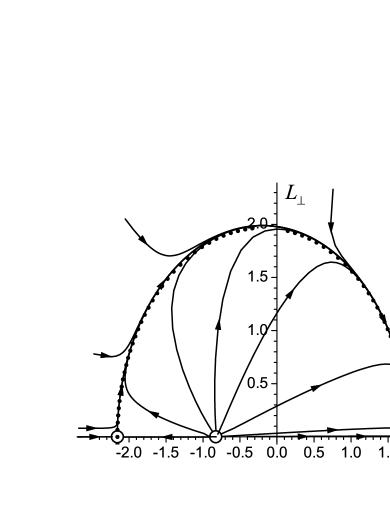
Рис. 1: The evolution of $L_{\bot}$ and $L_{z}$, calculated numerically for $J_{1}=J_{2}=2J_{12}$ and $S_{0}=1$ at $M=0.4$ and shown as a phase portrait. Singular points are shown with circles, and the separatrix is shown as a dotted line.

Thus, the exact solution of the full system of equations of motion for sublattice spins in the exchange approximation shows the existence of two qualitatively different regimes. The character of the evolution is mainly determined by the initial value of the magnetization $M$, which is conserved in the exchange approximation. For large $M>M_{c}$, as well as for all $M$ and the initial value $L_{z}(0)>0$, a longitudinal relaxation occurs, as studied previously in [16] . For $M<M_{c}$, approximately the same behavior is also retained for negative $L_{z}(0)$, provided that $L_{z}(0)>-L_{2}$. In all those cases, there is a special solution of the form $L_{z}=L_{z}(t)$ which leads to the equilibrium, and even for a nonzero (but small) value of the transversal initial deviation $L_{\bot}(0)$ the value of $L_{\bot}$ remains small in the process of relaxation. However, the situation is changed dramatically, if the initial value enters the region of the unstable node situated around $L_{z}\simeq-L_{2}$ ($L_{z}\simeq 0.83$ in Fig. 1). As seen in Fig. 1, in the vicinity of this point and to its left, even small initial values of $L_{\bot}$ increase with time. In this case, in a wide range of the initial conditions all trajectories in the $(L_{z},L_{\bot})$ plane tend to the separatrix which connects the saddle point and the unstable node; the values of $L_{\bot}$ are not small at the separatrix. In this way, strongly nonlinear evolution regimes with $L_{\bot}\sim L_{z}\sim 1$ become possible. The solution with $L_{\bot}\neq 0$ at $M\neq 0$ is of the precession type, i.e., for the initial condition with $L_{z}<-L_{2}$ approaching equilibrium is accompanied by the growth of the precession amplitude of ${\rm{\bf L}}$, at the constant precession frequency $\hbar\omega=J_{12}M$, so that ${\rm{\bf L}}=L_{z}{\rm{\bf e}}_{z}+L_{\bot}({\rm{\bf e}}_{x}\cos\omega t+{\rm{\bf e}}_{y}\sin\omega t)$. It should be remarked that the experimentally observed time dependence of the sublattice magnetizations in the time interval between $0.5$ and $3$ ps shows some non-monotonic behavior at the background of a smooth magnetization change, which resembles oscillations with the period of about $0.3$ ps, see Fig. 2 of Ref. [13] . The results of numerical simulation of this process, reported in the same work [13] , did not show such a behavior, but oscillations were found in recent numerical studies [888] .

Taking into account the transversal spin deviations in the process of evolution may be important for understanding the recent experiment on TbFeCo alloy [TbFe] . An obvious difference between this material and GdFeCo is the presence of a strong easy-axis anisotropy, but it is clear that such anisotropy should not affect a purely longitudinal evolution. Despite that, spin switching characteristic for GdFeCo was not observed in TbFeCo, although the initial reduction of the sublattice magnetizations was roughly the same as in the GdFeCo experiment. Of course, there could be other reasons for such a different behavior, e.g., the presence of unquenched orbital moment of Tb, but the detailed analysis of this problem is beyond the scope of the present paper.

This work is partly supported by the joint Grant 0113U001823 of the Russian Foundation for Fundamental Research and the Presidium of the National Academy of Science of Ukraine, and by the joint Grant $\Phi$53.2/045 of the Russian and Ukrainian Foundations for Fundamental Research.

- (1) E. Beaurepaire, J.-C. Merle, A. Daunois, and J.-Y. Bigot, Phys. Rev. Lett. 76, 4250 (1996).
- (2) A. Kirilyuk, A. V. Kimel, and Th. Rasing, Rev. Mod. Phys. 82, 2731 (2010).
- (3) M. Battiato, K. Carva, P. M. Oppeneer, Phys. Rev. Lett. 105, 027203 (2010); D. Rudolf, C. La-O-Vorakiat, M. Battiato et. al , Nature Comm. 3, 1037 (2012); M. Battiato, K. Carva, and P. M. Oppeneer, Phys. Rev. B 86, 024404 (2012)
- (4) I. Radu, K. Vahaplar, C. Stamm et. al , Nature (London) 472, 205 (2011).
- (5) T. A. Ostler, J. Barker, R. F. L. Evans et. al, Nature Commun. 3, 666 (2012).
- (6) L. Le Guyader, S. El Moussaoui, M. Buzzi, R. V.Chopdekar, L. J. Heyderman, A.Tsukamoto, A.Itoh, A.Kirilyuk, Th.Rasing, A. V.Kimel, and F.Nolting, Appl. Phys. Lett 101, 022410 (2012).
- (7) A. R. Khorsand, M. Savoini, A. Kirilyuk, A.V. Kimel, A. Tsukamoto, A. Itoh, and Th. Rasing, Phys. Rev. Lett. 108, 127205 (2012)
- (8) J. H. Mentink, J. Hellsvik, D. V. Afanasiev, B. A. Ivanov, A. Kirilyuk, A. V. Kimel, O. Eriksson, M. I. Katsnelson, and Th. Rasing, Phys. Rev. Lett. 108, 057202 (2012).
- (9) L. D. Landau and E. M. Lifshitz, To the theory of magnetic permeability of ferromagnetic bodies, In: L. D. Landau, The collection of works, Vol.1, p. 128 (Nauka, Moscow 1969) [in Russian].
- (10) T. L. Gilbert, Phys. Rev. 100, 1243 (1955).
- (11) V. G. Bar’yakhtar, Zh. Eksp. Theor. Fiz. 87, 1501 (1984); Fiz. Tverd. Tela 29, 1317 (1987) [Sov. Phys. JETP 60, 863, (1984); Sov. Phys. Solid State 29, 754 (1987)].
- (12) Fiz. Nizkikh Temp. 11, 1198 (1985); Zh. Eksp. Theor. Fiz. 94, 196 (1988) [Sov. J. Low Temp. Phys. 11, 662 (1985); Sov. Phys. JETP 67, 757 (1988)].
- (13) V. G. Bar’yakhtar, B. A. Ivanov, T. K. Soboleva, and A. L. Sukstanskii, Zh. Eksp. Theor. Fiz. 91, 1454 (1986) [Sov. Phys. JETP 64, 857 (1986)]; V. G. Bar’yakhtar, B. A. Ivanov and K. A. Safaryan, Solid State Comm. 72, 1117 (1989); E. G. Galkina, B. A. Ivanov and V. A. Stephanovich, JMMM 118, 373 (1993); V. G. Bar’yakhtar, B. A. Ivanov, A. L. Sukstanskii and E. Yu. Melekhov, Phys. Rev. B 56, 619 (1997).
- (14) V. López-Flores, N. Bergeard, V. Halté et. al, Phys. Rev. B 87, 214412 (2013).
- (15) V. N. Krivoruchko and D. A. Yablonskii, Zh. Eksp. Theor. Fiz. 74, 2268 (1978) [Sov. Phys. JETP 47, 1179 (1978) ]; Fiz. Tverd. Tela 21, 1502 (1979) [in Russian].
- (16) U. Atxitia, T. Ostler, J. Barker, R. F. L. Evans, R. W. Chantrell, and O. Chubykalo-Fesenko, Phys. Rev. B 87, 224417 (2013).
- (17) A. R. Khorsand, M. Savoini, A. Kirilyuk, A.V. Kimel, A. Tsukamoto, A. Itoh, and Th. Rasing, Phys. Rev. Lett. 110, 107205 (2013).