THE Spitzer-SOUTH POLE TELESCOPE DEEP FIELD: SURVEY DESIGN AND IRAC CATALOGS

Abstract

The Spitzer-South Pole Telescope Deep Field (SSDF) is a wide-area survey using Spitzer’s Infrared Array Camera (IRAC) to cover 94 deg² of extragalactic sky, making it the largest IRAC survey completed to date outside the Milky Way midplane. The SSDF is centered at ($\alpha,\delta)=($23:30,$-$55:00), in a region that combines observations spanning a broad wavelength range from numerous facilities. These include millimeter imaging from the South Pole Telescope, far-infrared observations from Herschel/SPIRE, X-ray observations from the XMM XXL survey, near-infrared observations from the VISTA Hemisphere Survey, and radio-wavelength imaging from the Australia Telescope Compact Array, in a panchromatic project designed to address major outstanding questions surrounding galaxy clusters and the baryon budget. Here we describe the Spitzer/IRAC observations of the SSDF, including the survey design, observations, processing, source extraction, and publicly available data products. In particular, we present two band-merged catalogs, one for each of the two warm IRAC selection bands. They contain roughly 5.5 and 3.7 million distinct sources, the vast majority of which are galaxies, down to the SSDF 5$\sigma$ sensitivity limits of 19.0 and 18.2 Vega mag (7.0 and 9.4 $\mu$Jy) at 3.6 and 4.5 $\mu$m, respectively.

1 Introduction

The large-scale distribution of both baryonic and dark matter and the physical laws that govern their evolution are fundamental to cosmology. Observations of the cosmic microwave background constrain the baryon-to-matter ratio to be $\sim$16% (Story et al.  2012; Hinshaw et al.  2013; Planck Collaboration XVI 2013). But observations of galaxy clusters have special advantages for understanding the abundance and distribution of matter, because 1) clusters are large enough that they are expected to retain the cosmic fraction of baryons, and 2) clusters are among the few astrophysical objects for which the three dominant forms of matter can be observed, namely: the gas mass ($M_{\rm gas}$), the stellar mass ($M_{\rm star}$), and the dark matter mass ($M_{\rm DM}$). However, observations of the matter distribution in clusters as a function of physical scale and mass have typically been constrained only at low redshift ($z<0.5$).

At low redshift, the best measurements of the baryon faction to date account for $\sim$80% of the cosmic value (for a recent review, see Kravtsov et al.  2009). The baryonic mass is dominated by an intra-cluster gas component (Vikhlinin et al.  2006; Arnaud et al.  2007; Sun et al.  2009), with stars and galaxies typically contributing roughly one-tenth as much mass (Gonzalez et al.  2007; Giodini et al.  2009; Lin et al.  2012). However, the stellar mass fraction has also been found to be a strong function of cluster mass, with the stellar-to-gas fraction decreasing from $\sim$0.25 to 0.05 from groups ($\sim 5\times 10^{13}M_{\odot}$) to massive clusters ($\sim 10^{15}M_{\odot}$). This can be interpreted to mean that star formation is much more efficient in the lower-mass groups compared to rich clusters (e.g., Muzzin et al.  2012).

In contrast with observations, simulations generally predict that the stellar fraction is approximately constant with cluster mass, and over-predict the amount of stars formed by a factor of $\sim$2–5 in massive clusters (e.g., Kravtsov et al.  2009). More recently, simulations have tried to evoke various types of astrophysical feedback (e.g., supernovae and active galactic nuclei) to suppress star formation and match the observed stellar and intracluster medium fraction, with some success (e.g., Planelles et al.  2012; Battaglia et al.  2013).

Some of the fundamental questions about galaxy and structure formation that still await resolution include:

1. Why is the baryon fraction in cluster gas less than the universal average? Are the missing cluster baryons in stars? Do the observations underestimate the total diffuse stellar mass in the form of intra-cluster light?

2. How do the relationships between cluster gas, dark matter, and stars evolve with redshift? Given that clusters are built hierarchically from mergers of lower-mass groups, in the simplest scenario one might expect these relations to be significantly steeper at higher redshift.

3. What is the radial distribution of the baryonic components as a function of M_DM and redshift?

4. What is the assembly history of baryons in the most massive structures?

Spitzer’s Infrared Array Camera (IRAC; Fazio et al.  2004a) has already been used to carry out several relatively wide-area extragalactic surveys, e.g., SWIRE (Lonsdale et al. 2003), SDWFS (Ashby et al. 2009), and SERVS (Mauduit et al. 2012), covering more than $70\,$ deg² all together. Among many other things, datasets such as these provide an efficient means to identify statistical samples of galaxy clusters down to low masses even at high redshifts (Eisenhardt et al.  2008; Muzzin et al.  2009; Papovich et al.  2010; Stanford et al.  2012). However, the cluster searches carried out to date are not fully characterized in terms of purity, completeness, or mass proxies (via comparison with cluster samples identified at other wavelengths), hindering interpretations that depend upon either cluster mass or ensemble properties.

Here we describe a new wide-area IRAC survey that will make it possible to combine groundbreaking datasets from the South Pole Telescope and XMM with coextensive infrared imaging to address the questions posed above. We call this the Spitzer-South Pole Telescope Deep Field (SSDF) survey. The SSDF depth and coverage are compared to those of other major IRAC survey projects in Figure 1. The combination of infrared, millimeter, and X-ray data provides a unique opportunity to simultaneously calibrate the IRAC search techniques via comparison with Sunyaev-Zel’dovich (SZ) and X-ray cluster samples, and to robustly determine the cluster selection functions at the depths simultaneously probed by the three techniques. A limitation of the present generation of X-ray and SZ surveys is that they lack the sensitivity at high redshift to identify clusters down to $10^{14}$ M_⊙ and below, as is possible with IRAC. Reaching these mass scales at higher redshifts is critical for understanding the assembly history of the present day cluster population, as these low-mass systems are the direct progenitors of typical present-day clusters, like Virgo. The IRAC component is essential for finding the lowest-mass clusters at all redshifts $z>0.5$ and for determining photometric redshifts for complete galaxy samples (Brodwin et al.  2006). It is also vital for determining galaxy luminosities and sizes within clusters (e.g., Brodwin et al.  2010), and for estimating the stellar masses of all clusters found by any selection technique (e.g., Eisenhardt et al.  2008). Because the SSDF offers an opportunity to bring the X-ray and millimeter imaging together with wide-field IRAC data, it is poised to become a uniquely valuable resource for galaxy cluster research.

In this contribution, we describe the Spitzer/IRAC survey: the field, the observations, the reduction, and in particular the resulting catalogs that will serve as the basis for future work aimed at addressing the unresolved questions surrounding the distribution of baryons in the Universe. This paper is organized as follows: Section 2 describes the SSDF field and previous observations relevant to galaxy cluster science. Section 3 discusses the details of the SSDF observing strategy and data reduction, and Section 4 describes the source identification, photometry, and validation. Section 5 describes the SSDF catalogs. In Section 6 we present preliminary results, including wide-field infrared number counts and the infrared color distribution of IRAC-detected galaxies. We summarize in Section 7. Unless otherwise stated, all magnitudes are given in Vega-relative terms. Users can convert to the AB scale by adding 2.792 and 3.265 mag to the cataloged 3.6 and 4.5 $\mu$m magnitudes, respectively.

2 The Spitzer-South Pole Telescope Deep Field

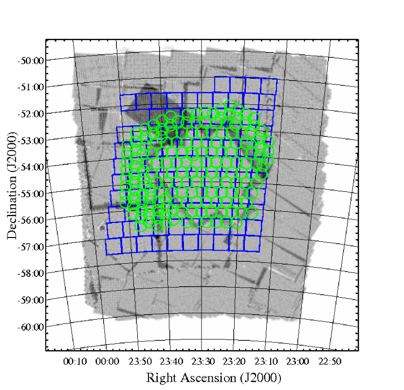
Figure 2: The SSDF depth of coverage at 4.5 $\mu$m (greyscale) including all observations taken through 2013 February. The linear stretch ranges from zero (white) to 15 (black). Most of the field is covered to the designed depth ($4\times 30$ s). The coverage at 3.6 $\mu$m is very similar to that shown here. Blue squares indicate tiles covered by $griz$ observations from the Blanco Cosmology Survey (Desai et al.  2012). Green circles indicate XMM pointings from the XXL survey, covering a total of 25 deg² to a depth of 10 ks. A full-resolution version of this figure is available in the version of this article published in the ApJS.

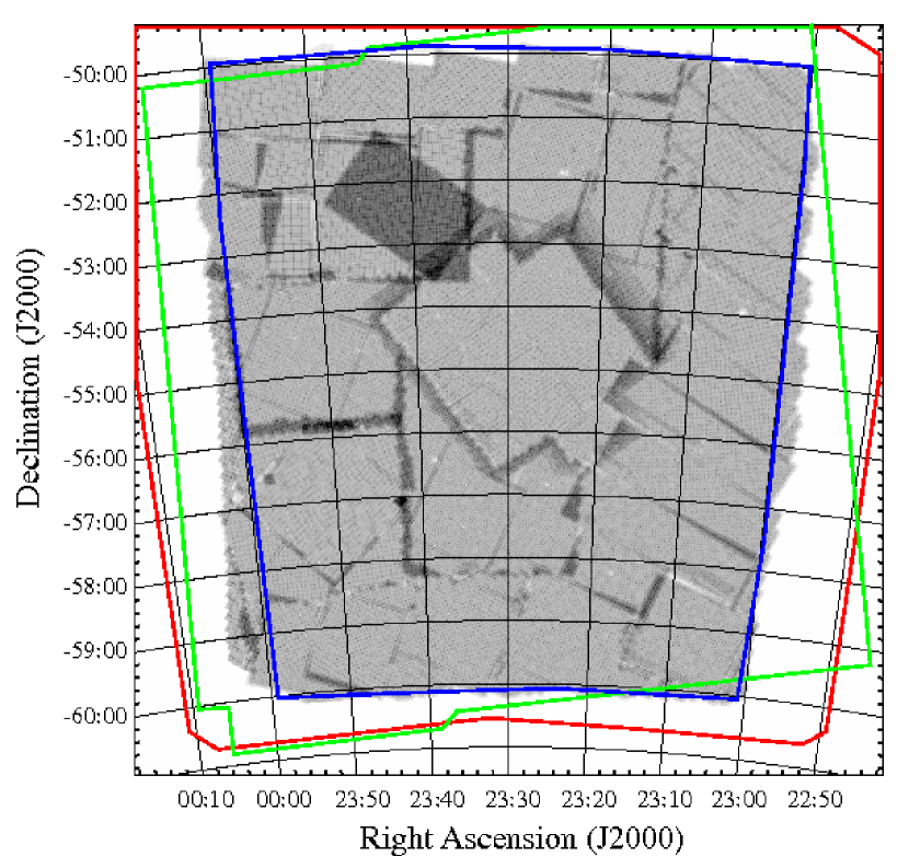
Figure 3: As Figure 2, but showing the boundaries of the coextensive coverage at long wavelengths. The extent of coverage obtained via SPT imaging at 1.4, 2, and 3 mm (the SPT deep field) is shown in red, while the Herschel/SPIRE far-infrared imaging is outlined in green, and the ATCA 16 cm imaging is outlined in blue. A full-resolution version of this figure is available in the version of this article published in the ApJS.

We carried out our survey in a field that benefits from an abundance of supporting data from X-ray to radio wavelengths, and which has extremely low levels of Galactic dust emission, being among the cleanest 1% of contiguous 100 deg² regions on the sky as measured in the 100 $\mu$m IRAS map (Finkbeiner et al. 1999). The SSDF is centered at $(\alpha,\delta)=(23$:30,$-$55:00). The relationship of the SSDF coverage to that of coincident surveys at other wavelengths is shown in Figures 2 and 3, is summarized in Table 1, and is described in detail below.

Their sensitivity to baryons in the intracluster medium makes X-ray observations particularly important for the study of galaxy clusters, and the XMM mission carried out a large-area survey specifically designed to be very sensitive to clusters. This is the XXL survey (Pierre et al.  2011), of which a 25 deg² portion is located in the SSDF. The XXL survey was performed in 2011–2013 with 10 ks integrations per pointing, and the resulting cluster catalogs are now being confirmed via spectroscopic followup programs at the AAT, NTT, and VLT (M. Pierre et al., in prep.) The XXL survey is the largest deep-wide X-ray survey for galaxy clusters in existence, with an area five times greater than existing XMM surveys and sensitivity sufficient to study clusters beyond $z=1$ down to masses of $\sim 10^{14}$ M_⊙. The cross-comparision between the infrared and X-ray cluster catalogs will provide unique information about the purity and completeness of the samples as well as on the physics of high-redshift clusters.

The entire SSDF was also imaged at far-infrared wavelengths in 2011 with Herschel’s Spectral and Photometric Imaging REceiver (SPIRE; Griffin et al.  2010). The SPIRE imaging reaches 1$\sigma$ depths of roughly 10 mJy beam^-1 at 250, 350, and 500 $\mu$m. The SPIRE data will be very useful for studies of submm galaxies and for cross-correlation studies involving Cosmic Microwave Background lensing maps (e.g., Holder et al.  2013), and should probe ULIRG activity in galaxy clusters. Shallow infrared imaging is already available from the all-sky WISE survey (Wright et al.  2010), which reaches 1 and 6 mJy at 12 and 22 $\mu$m, respectively. In the radio, the full field is being imaged with the Australia Telescope Compact Array (ATCA) at 16 cm down to 40 $\mu$Jy beam^-1 with a 7″ beam.

In the visible/near-infrared regime, the SSDF already has extensive coverage from both completed and ongoing surveys. The Blanco Cosmology Survey (Desai et al.  2012; L. Bleem et al.  in preparation) surveyed $\sim$30 deg² of the SSDF in the $griz$ bands down to roughly 23 AB mag (10 $\sigma$). The ongoing Dark Energy Survey will obtain $griz$ imaging down to approximately 24 AB mag (10$\sigma$) over a large area that includes the entire SSDF. In the near-infrared, Data Release 1 of the VISTA Hemisphere Survey (McMahon et al. , in preparation) has already covered nearly the entire field in $JHK$ to 5$\sigma$ limits of 21.2, 20.8, and 20.2 AB mag.

Roughly 12 deg² in the center of the SSDF were observed with Spitzer/IRAC in Cycle 4 (PI Stanford, PID 40370) with three dithered 30 s exposures. These observations were incorporated into the SSDF and are hereafter referred to as the S-BCS (Spitzer-Blanco Cosmology Survey). Because it was obtained during Spitzer’s cryogenic mission, the S-BCS dataset includes exposures at 5.8 and 8.0 $\mu$m, although those two long-wavelenth bands were not analyzed as part of the present work because they are significantly less sensitive than our new IRAC imaging.

The SSDF has already been fully covered at 95, 150, and 220 GHz to 1$\sigma$ depths of 2, 1, and 3 mJy beam^-1, respectively by the South Pole Telescope (SPT) during its survey of more than 2500 deg² of the southern sky (Carlstrom et al. 2011; Story et al. 2012). The SPT provides an efficient means to detect high-redshift dusty galaxies (e.g., Vieira et al. 2013), but it is particularly effective for identifying galaxy clusters via the Sunyaev-Zel’dovich effect (SZ; Sunyaev & Zel’dovich 1972). The SZ selection technique is relatively insensitive to cluster redshift, so the SPT observations are capable of identifying galaxy clusters out to great distances (e.g., Reichardt et al.  2013). Over the next four years, even deeper observations by SPTpol (Austermann et al.  2012), which has already imaged this field to nearly twice the depth of the larger SPT survey (Story et al. 2012) will further improve the quality and depth of the millimeter data in this field. Its southern location means that it is well-placed for followup observations with the Atacama Large Millimeter/Submillimeter Array, and is a promising candidate for selection as one of the Large Synoptic Survey Telescope deep drilling fields.

3 Observations and Data Reduction

3.1 Mapping Strategy

The observing plan drew heavily on our team’s prior experience with the IRAC Shallow Survey (Eisenhardt et al.  2004). The observations were arranged to account for and smoothly extend the pre-existing IRAC coverage from the S-BCS (3$\times$30 s depth over 12 deg²). They also had to accommodate the position angle (PA) constraints of the two observing windows opening six months apart as well as the SSDF boundaries. The SSDF lies between Declinations $-50$ deg and $-60$ deg, and from Right Ascension 23 hr to slightly east of 0 hr (Figure 2). To accommodate these constraints, the SSDF was covered by Astronomical Observation Requests (AORs) having coverage footprints of various (sometimes irregular) shapes and sizes. When possible, standard IRAC grids were used to cover $\sim 1\times$1 deg² areas in four passes, each pass obtaining a single 30 s exposure per position. Around the edges of and in between these grids, we designed AORs in fixed cluster mode so as to optimally cover irregular areas. Like the AORs covering areas having more regular shapes, these gerrymandered observations were also organized into groups of four single-pass AORs to cover each area, with a single 30 s exposure obtained in each pass. In any one area, the four AORs were obtained over the course of a two-day window. The goal was to achieve uniform coverage to the greatest extent possible.

Each AOR required 1–6 hr to execute, ensuring at least 1 hr between successive observations of each sky position. For typical asteroid motions of 25″ hr^-1, asteroids will move distances much greater than the IRAC point spread function between AORs. The four observations of each sky position therefore allowed asteroids to be excluded from the final mosaics with standard outlier rejection techniques.

Our mapping strategy was to dither the exposures on small scales, and offset by one-third of an IRAC field of view between successive passes through each AOR group. This provided inter-pixel correlation information on both small and large scales. Our observing strategy is therefore very robust against bad rows/columns, large scale cosmetic defects on the array, after-images resulting from saturation due to bright stars, variations in the bias level, and the color dependence of the IRAC flat-field across the array (Quijada et al.  2004).

Although the four-AOR observations of specific areas were performed consecutively, spacecraft visibility constraints meant that coverage of the full SSDF had to be accumulated in separate campaigns spaced roughly six months apart. These took place in 2011 July-August, 2012 January-February, 2012 July-September, and 2012 December-2013 February. Because adjacent regions were inevitably observed at slightly different PAs, obvious and irregular coverage gaps were evident between adjacent mapping AOR sets as the observations accumulated. These were covered in the latter two epochs with cluster-mode AORs during which the exposures were placed to fill the coverage gaps as smoothly as possible given the spacecraft visibility limits and position angles. Like the AORs executed earlier, these irregular cluster-mode AORs were done in sets of single-pass rasters intended to accumulate a total of four dithered 30 s exposures everywhere.

3.2 Data Reduction

To the maximum extent possible, identical reduction procedures were applied to all SSDF and S-BCS data so as to ensure uniform data quality throughout the field. The data reduction was based on version S18.18.0 of the IRAC Corrected Basic Calibrated Data (cBCD) exposures for the first SSDF campaign; version S19.1.0 was used for all other, later campaigns. The cBCD data were used because some of the salient instrument artifacts (e.g., multiplexer bleed) are automatically corrected by the cBCD pipeline. Other artifacts (e.g., scattered light) are flagged in the cBCD pipeline-adjusted pixel masks for each frame. Both features of the cBCD data make them optimal for our purposes.

To remove slowly-decaying residual images from unrelated observations of bright objects, all 3.6 and 4.5 $\mu$m cBCD frames were object-masked and median-stacked on a per-AOR basis. The resulting stacked images (presumed to represent blank sky) were visually inspected and subtracted from individual cBCDs within each AOR. This created sky-subtracted versions of the cBCDs that were free of long-term residual images arising from prior observations of bright sources. Residual images with short decay times arising from observations of bright stars during the SSDF observations themselves were not addressed by this method, however. Pixels flagged as potentially contaminated with such residuals by the IRAC pipeline were masked. The sky-subtracted cBCDs were then examined individually and processed using custom software routines to correct column-pulldown effects associated with bright sources. The code, known as the “Warm-Mission Column Pulldown Corrector,” is publicly available at the Spitzer Science Center.

After these preliminaries, the SSDF exposures and the coincident IRAC imaging from the S-BCS were mosaiced with IRACproc (Schuster et al. 2006). IRACproc augments the capabilities of the standard IRAC reduction software (MOPEX) by calculating the spatial derivative for each image pixel and adjusting the clipping algorithm accordingly. Pixels where the derivative is low (in the field) are clipped more aggressively than are pixels where the spatial derivative is high (point sources). This avoids downward biasing of point source fluxes in the output mosaics that might otherwise occur because of the slightly undersampled IRAC point spread function (PSF). The software was configured to automatically flag and reject cosmic ray hits based on pipeline-generated masks together with the adjusted sigma-clipping algorithm for spatially coincident pixels.

The IRAC mosaics were organized into pairs of coextensive tiles each covering roughly $2\times 1$ deg² sub-fields at both 3.6 and 4.5 $\mu$m. A total of 46 tiles were required to cover the full SSDF. The IRAC coverage and the tile dimensions and locations are defined in Figure 4 and Table 2. By construction, the World Coordinate Systems of all SSDF tile pairs are tied to the coordinates of objects in the Two Micron All Sky Survey Point Source Catalog (2MASS, Skrutskie et al.  2006), and are in perfect pixel-by-pixel registration.

The resulting 92 final mosaics/coverage map pairs (one pair per tile per band), are publicly available from the Exploration Science Programs webpage at the Spitzer Science Center. All SSDF mosaics were built with 0$\farcs$6 pixels and have units of MJy sr^-1.

4 Source Extraction and Photometry

4.1 Source Identification

We detected and photometered sources in the SSDF mosaics with SExtractor (ver. 2.8.6; Bertin & Arnouts 1996). SExtractor is well-suited to the relatively sparse SSDF mosaics, where there are numerous source-free pixels available for robust sky background estimation. We adopted the SExtractor parameter settings shown in Table 3. The coverage maps constructed by IRACproc were used as detection weight images. Custom flag images were constructed to identify and exclude all mosaic pixels covered by fewer than two exposures.

Photometry was measured within nine apertures having diameters ranging from 2″ to 10″ in 1″ increments, plus two additional apertures of diameter 15″ and 24″, or eleven apertures in all. By comparing photometry measured in the 24″ aperture (i.e., the aperture adopted by the Instrument Team as the fiducial photometric aperture for IRAC) to that in all other apertures for well-detected, isolated sources, we obtained empirical estimates of the aperture corrections, which are given in Table 4. We also obtained MAG_AUTO magnitudes, for which SExtractor measures fluxes interior to elliptical apertures having sizes and orientations determined using the second-order moments of the light distribution measured above the isophotal threshold. We compared the MAG_AUTO photometry to the corrected-to-total aperture magnitudes and found that the MAG_AUTO estimates were systematically fainter by roughly 0.05 mag. In other words, the corrected aperture magnitudes are consistent with each other, but the MAG_AUTO measurements are 0.05 mag fainter on average.

We used SExtractor in dual-image mode. In this configuration, sources are detected, their centers are located, and their apertures are defined in one image, and subsequently photometry is carried out in another image using those pre-established apertures and source centroids. The dual-image approach forces SExtractor to measure the emission from all sources over identical areas in both bands, ensuring that the resulting photometry will yield accurate source colors. SExtractor was configured to define a source as a set of four or more connected pixels each lying 0.5$\sigma$ above the estimated background. We first used the 4.5 $\mu$m mosaics as the detection images; both the 3.6 and 4.5 $\mu$m mosaics were used in turn as the photometry images. The process was followed in all 46 tiles covering the SSDF, resulting in 46 pairs of single-band catalogs.

Because the source extraction was performed in dual-image mode, the separate 3.6 and 4.5 $\mu$m SExtractor catalog pairs generated for each of the two selection bands were in line-by-line registration. We generated band-merged catalogs by combining photometry from these catalog pairs for all SSDF tiles. The band-merged, tile-based catalogs were trimmed to exclude overlapping regions at the tile boundaries given in Table 2, and all aperture photometry was corrected to total magnitudes using the empirical aperture corrections from Table 4. A full-field catalog covering the entire SSDF was then created by combining the trimmed, band-berged, aperture-corrected photometry from all tiles. We chose to include the corrected 4″ and 6″ diameter aperture magnitudes in the final catalogs, along with the SExtractor MAG_AUTO magnitudes.

Finally, the above process was repeated using the 3.6 $\mu$m mosaics as the detection images. The result is a pair of full-field band-merged SSDF catalogs – one selected at 3.6 $\mu$m, and another selected at 4.5 $\mu$m.

4.2 Survey Depth, Completeness, and Astrometric Reliability

4.2.1 Survey Depth and Completeness Estimation

We used a Monte Carlo approach to estimate the survey completeness and sensitivity by placing numerous simulated sources in the SSDF mosaics at random locations and then photometering them in an identical manner to that used for the original mosaics. Specifically, we inserted simulated objects in both the 3.6 and 4.5 $\mu$m mosaics for five different SSDF tiles (labeled SSDF1.6, 2.4, 2.6, 3.2, and 3.5 in Figure 4) chosen as representative of the range of IRAC depths of coverage that we obtained. The total area in which the simulated sources were inserted and subsequently photometered therefore samples roughly 10.6 deg² of the total survey field.

The simulated sources were randomly assigned magnitudes between 10 and 21 Vega mag. Hundreds of simulated sources in this range were simultaneously placed at random locations in each of the five tiles employed for this purpose. The number of simulated sources inserted at one time was restricted to a small percentage of the total number of objects apparent in the field, so as to avoid artificially-induced source confusion effects. Nonetheless, because the simulated sources were allowed to fall anywhere in their respective tiles, including atop real sources, the simulations do account realistically for the effects of source confusion. The process was iterated, so that a total population of 20,000 simulated sources was ultimately analyzed in each of the 0.5 mag-wide bins we constructed to span the magnitude range we considered.

After processing the modified mosaics with SExtractor in exactly the same way as was done for the original mosaics, the resulting catalogs were compared to determine the completeness as a function of magnitude. The comparison was performed in catalog space with MAG_AUTO magnitudes using a simple position-matching criterion. An additional constraint was imposed, requiring that a valid detection of a simulated source had to yield a measured magnitude that fell within 0.5 mag of its a priori known magnitude to account for source confusion. This procedure was repeated in both bands for all five tiles tested. The results are given in Table 5 and shown in Figure 5.

The SSDF catalogs include only sources with aperture-corrected (total) magnitudes brighter than the achieved sensitivity levels in at least one of the two SSDF bands. We defined the SSDF sensitivity as the magnitude at which the empirical uncertainty in the SExtractor-estimated fluxes reached approximately the 5$\sigma$ level (0.2 mag). This occurred at [3.6]=19.0 mag (7.0 $\mu$Jy) and [4.5]=18.2 mag (9.4 $\mu$Jy) for 4″ diameter apertures, similar to the sensitivity reported by Eisenhardt et al.  (2004) for the first IRAC survey of Boötes: [3.6]=19.1 mag and [4.5]=18.3 mag. The SSDF thus achieves 5$\sigma$ sensitivities similar to those predicted by the online Sensitivity Performance Estimation Tool (SENS-PET): [3.6]=19.2 mag and [4.5]=18.6 mag assuming low background conditions.

4.2.2 Astrometric Reliability

To estimate the accuracy of the SSDF astrometry, we compared SSDF IRAC positions of bright but unsaturated sources to those in the 2MASS Point Source Catalog (Skrutskie et al.  2006). We performed a search within 1″ of the positions of IRAC sources to identify their 2MASS counterparts. The distributions of coordinate offsets for the 3.6 and 4.5 $\mu$m sources are shown in Figure 6. The astrometric discrepancies are small compared to the size of a SSDF pixel: the mean difference (SSDF$-$2MASS) was just $-0\farcs 15\pm 0\farcs 26$ in Right Ascension and $0\farcs 03\pm 0\farcs 23$ in Declination. The total radial uncertainties are therefore $0\farcs 15$ (1$\sigma$) relative to 2MASS. This is about one-fourth of an SSDF mosaic pixel, and less than one-tenth of the full width at half maximum of the IRAC PSF in either band. This is comparable to the astrometric precision obtained in other Spitzer/IRAC surveys, e.g., SDWFS (Ashby et al. 2009).

5 SSDF Catalogs

Both versions of the band-merged SSDF catalogs are presented here, one for each of the two selection bands (3.6 and 4.5 $\mu$m). The catalogs contain a total of $5.5\times 10^{6}$ and $3.7\times 10^{6}$ 3.6 $\mu$m- and 4.5 $\mu$m-selected sources, respectively, down to the 5$\sigma$ detection thresholds. The formats of the two catalogs are identical and are defined in Table 6. All aperture magnitudes in both catalogs have been corrected to total magnitudes using the aperture corrections given in Table 4. The catalogs also contain MAG_AUTO total magnitude estimates. All photometric estimates are provided with 1$\sigma$ uncertainty estimates generated by SExtractor, and are also given as flux densities in units of $\mu$Jy. In addition to the photometry, the SSDF catalog provides a number of SExtractor-derived descriptors for each source as measured in the selection band, 3.6 or 4.5 $\mu$m as appropriate (Table 6).

6 Discussion

The measured colors of celestial sources reflect their underlying nature, albeit after being folded through the detection/selection process. The IRAC colors for all sources listed in the two SSDF catalogs are shown in Figure 7. The color distributions are broadly consistent with what is seen typically with IRAC at these flux levels, e.g., Ashby et al.  (2009). For example, the faintest SSDF sources (those fainter than [3.6]=[4.5]=17.5 Vega mag) are systematically and significantly redder than brighter SSDF sources. This is because the surface density of relatively red extragalactic sources increases quickly below 17 mag, while the contribution from Galactic stars, which are relatively blue in the IRAC bands, flattens out (e.g., Fazio et al. 2004b).

The differential IRAC number counts in the SSDF are given in Table 7 and Figure 8, after applying appropriate corrections for incompleteness based on the empirical estimates in Table 5. Although the SSDF catalogs contain many sources brighter than 10 mag, these are not shown in the source counts because they are saturated in the IRAC mosaics. Nonetheless the SSDF counts are broadly consistent with counts measured earlier by, e.g., Ashby et al.  (2009) and Fazio et al.  (2004b), over the magnitude range covered by the SSDF catalogs. At bright flux levels, the SSDF counts are slightly elevated with respect to SDWFS. We have examined the SSDF mosaics at the locations of sources in the affected magnitude ranges, and find that virtually all are pointlike. This is consistent with a picture in which these sources are due to Milky Way stars, seen along a line of sight that is closer in both latitude and longitude ($\ell,b)=(325,-58)$ to the Galactic center than is SDWFS ($\ell,b)=(60,+67)$. This is borne out by the consistency between the DIRBE model Milky Way star counts and the bright IRAC SSDF counts shown in Figure 8.

In the 30 s exposures used to construct the SSDF mosaics, sources brighter than $\sim$10 Vega mag in either IRAC band are saturated. Users of the SSDF catalogs are cautioned against uncritical usage of photometry for sources brighter than [3.6]=[4.5]=11.5 Vega mag. Objects that are truly as bright as this will be well-detected in any case by the two short-wavelength WISE bands.

7 Summary

We have carried out an infrared survey of nearly 100 deg² with the warm IRAC aboard Spitzer for our Cycle 8 Spitzer Exploration program, the Spitzer-South Pole Telescope Deep Field survey. With its combination of uniform depth in two infrared bands and wide-area coverage, this project provides a unique resource for extragalactic research. It benefits from numerous coextensive observations spanning X-ray to radio wavelengths, in particular the deep imaging acquired by the South Pole Telescope at 1.4, 2, and 3 mm, and will therefore be of particular use for galaxy cluster science. The catalogs contain multiple photometric measurements for several million distinct IRAC sources down to the $5\sigma$ survey limits of 7.0 and 9.4 $\mu$Jy at 3.6 and 4.5 $\mu$m, respectively, and have been made publicly available to the astronomical community from the Spitzer Science Center.

Figure 1: Comparison of SSDF 3.6 µm depth and total area (solid circle) to other major Spitzer/IRAC extragalactic surveys. Open symbols indicate 1$\sigma$ point-source sensitivities for GOODS (Great Observatories Origins Deep Survey), EGS (Extended Groth Strip), E-CDFS (Extended Chandra Deep Field South), SpUDS (Spitzer Public Legacy Survey of UKIDSS Ultra-Deep Survey), SCOSMOS (Spitzer Deep Survey of HST COSMOS 2-Degree ACS Field), SERVS (Spitzer Extragalactic Representative Volume Survey), S-BCS (Spitzer-Blanco Cosmology Survey), SWIRE (Spitzer Wide-area Infrared Extragalactic Survey), the FLS (Spitzer First-Look Survey), SDWFS (Spitzer Deep, Wide-Field Survey), SEDS (Spitzer Extended Deep Survey), S-CANDELS (Spitzer-CANDELS), and the Spitzer-IRAC Equatorial Survey (SpIES). All sensitivities shown are based on low-background estimates made with the Spitzer Sensitivity and Performance Estimation Tool (SENS-PET) except for SpIES (which used a high-background estimate), and the SSDF and SEDS, which are measured from actual data.

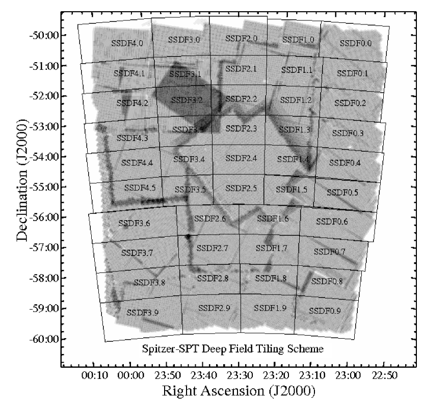
Figure 4: As Figure 2 but showing the tiling scheme used to define sub-regions of the SSDF in which mosaics were constructed as described in Section 3.2. The dark rectangle centered in tile SSDF3.2 at roughly ($\alpha,\delta)=($23:40,$-$52:30) is covered to $8\times 30$ s, twice the nominal SSDF depth. The original $3\times 30$ s S-BCS observations (now covered to $4\times 30$ s depth) are apparent as the irregular region of uniform coverage centered on tile SSDF2.4. A full-resolution version of this figure is available in the version of this article published in the ApJS.

Figure 5: Recovered fraction of simulated SSDF sources as a function of input magnitude, based on the simulations described in Section 4.2.

Figure 6: Coordinate offsets measured for IRAC-detected sources also detected in the 2MASS Point Source Catalog. The mean differences are $-0\farcs 15\pm 0\farcs 26$ in Right Ascension and $0\farcs 03\pm 0\farcs 23$ in Declination, giving a total radial uncertainty of just $0\farcs 15$ (1$\sigma$) relative to 2MASS, or less than one-tenth of the FWHM of the IRAC point spread function at 3.6 $\mu$m.

Figure 7: The color distributions of SSDF sources detected with greater than $5\sigma$ significance in both IRAC bands. All colors are measured from aperture-corrected 4″-diameter aperture photometry. Left panel: Colors for SSDF sources selected at 3.6 $\mu$m. The larger hatched histogram corresponds to the faintest sources, i.e., those fainter than $[3.6]=17.5$ mag. The brightest sources (those brighter than $[3.6]=16$ mag) are indicated with the smaller hatched histogram. Those of intermediate brightness are indicated with the open histogram. Right panel: As for the left panel, but for SSDF sources selected at 4.5 $\mu$m.

Figure 8: Differential source counts for the SSDF in the two IRAC bands. The 3.6 $\mu$m counts (left panel, solid triangles) are taken from the 3.6 $\mu$m-selected SSDF catalog, while the 4.5 $\mu$m counts (right panel, solid squares) are taken from the 4.5 $\mu$m-selected catalog. All counts shown here are based on SExtractor MAG_AUTO estimates for unsaturated sources and are corrected for the effects of incompleteness using the empirical estimates given in Table 5. The solid lines indicate the expected counts arising from Milky Way stars along the line of sight through the center of the SSDF at ($\alpha,\delta)=($23:30,$-$55:00) based on the DIRBE Faint Source Model at 3.5 and 4.9 $\mu$m in the left and right panels, respectively (Arendt et al. 1998; Wainscoat et al. 1992; Cohen 1993; 1994; 1995). The SSDF counts are similar to those measured in the narrower but more sensitive Spitzer Deep, Wide Field Survey (open symbols; Ashby et al.  2009), as discussed in Section 6.

Table 1: Available Survey Data in SSDF

Waveband	Origin	Depth
($\mu$m)		(5$\sigma$)
0.5-0.9 ($ugriz$)	Blanco Cosmology Survey	$\sim 1.0\,\mu$Jy	Bleem et al., in preparation
1.35 ($J$)	VISTA Hemisphere Survey	12.0 $\mu$Jy	McMahon et al., in preparation
1.65 ($J$)	VISTA Hemisphere Survey	17.4 $\mu$Jy	McMahon et al., in preparation
2.20 ($K$)	VISTA Hemisphere Survey	30.2 $\mu$Jy	McMahon et al., in preparation
3.6	Spitzer-SPT Deep Field	7.0 $\mu$Jy	This work
4.5	Spitzer-SPT Deep Field	9.4 $\mu$Jy	This work
12	WISE W3	1 mJy	Wright et al. (2010)
22	WISE W4	6 mJy	Wright et al. (2010)
250	Hershel/SPIRE	10 mJy	Holder et al. (2013)
350	Hershel/SPIRE	10 mJy	Holder et al. (2013)
500	Hershel/SPIRE	10 mJy	Holder et al. (2013)
1400	SPT	15 mJy	Story et al. (2012)
2000	SPT	5 mJy	Story et al. (2012)
3000	SPT	10 mJy	Story et al. (2012)

Note. — Depths of coverage for other surveys of the SSDF.

Table 2: SPT-Spitzer Tile Definitions

Tile	Right Ascension Range	Declination Range
	(Degrees, J2000)	(Degrees, J2000)
SSDF0.0	$\alpha\leq 348.23$	$-49.8\geq\delta>-51.0$
SSDF0.1	$\alpha\leq 348.00$	$-51.0\geq\delta>-52.0$
SSDF0.2	$\alpha\leq 348.00$	$-52.0\geq\delta>-53.0$
SSDF0.3	$\alpha\leq 348.00$	$-53.0\geq\delta>-54.0$
SSDF0.4	$\alpha\leq 348.00$	$-54.0\geq\delta>-55.0$
SSDF0.5	$\alpha\leq 348.00$	$-55.0\geq\delta>-56.0$
SSDF0.6	$\alpha\leq 348.75$	$-56.0\geq\delta>-57.0$
SSDF0.7	$\alpha\leq 348.75$	$-57.0\geq\delta>-58.0$
SSDF0.8	$\alpha\leq 348.75$	$-58.0\geq\delta>-59.0$
SSDF0.9	$\alpha\leq 348.75$	$-59.0\geq\delta>-60.2$
SSDF1.0	$348.23<\alpha\leq 351.00$	$-49.8\geq\delta>-51.0$
SSDF1.1	$348.00<\alpha\leq 351.00$	$-51.0\geq\delta>-52.0$
SSDF1.2	$348.00<\alpha\leq 351.00$	$-52.0\geq\delta>-53.0$
SSDF1.3	$348.00<\alpha\leq 351.00$	$-53.0\geq\delta>-54.0$
SSDF1.4	$348.00<\alpha\leq 351.00$	$-54.0\geq\delta>-55.0$
SSDF1.5	$348.00<\alpha\leq 351.00$	$-55.0\geq\delta>-56.0$
SSDF1.6	$348.75<\alpha\leq 352.49$	$-56.0\geq\delta>-57.0$
SSDF1.7	$348.75<\alpha\leq 352.45$	$-57.0\geq\delta>-58.0$
SSDF1.8	$348.75<\alpha\leq 352.38$	$-58.0\geq\delta>-59.0$
SSDF1.9	$348.75<\alpha\leq 352.35$	$-59.0\geq\delta>-60.2$
SSDF2.0	$351.00<\alpha\leq 354.00$	$-49.8\geq\delta>-51.0$
SSDF2.1	$351.00<\alpha\leq 354.00$	$-51.0\geq\delta>-52.0$
SSDF2.2	$351.00<\alpha\leq 354.00$	$-52.0\geq\delta>-53.0$
SSDF2.3	$351.00<\alpha\leq 354.00$	$-53.0\geq\delta>-54.0$
SSDF2.4	$351.00<\alpha\leq 354.00$	$-54.0\geq\delta>-55.0$
SSDF2.5	$351.00<\alpha\leq 354.00$	$-55.0\geq\delta>-56.0$
SSDF2.6	$352.49<\alpha\leq 356.25$	$-56.0\geq\delta>-57.0$
SSDF2.7	$352.45<\alpha\leq 356.25$	$-57.0\geq\delta>-58.0$
SSDF2.8	$352.38<\alpha\leq 356.25$	$-58.0\geq\delta>-59.0$
SSDF2.9	$352.35<\alpha\leq 356.25$	$-59.0\geq\delta>-60.2$
SSDF3.0	$354.00<\alpha\leq 357.00$	$-49.8\geq\delta>-51.0$
SSDF3.1	$354.00<\alpha\leq 357.00$	$-51.0\geq\delta>-52.0$
SSDF3.2	$354.00<\alpha\leq 357.00$	$-52.0\geq\delta>-53.0$
SSDF3.3	$354.00<\alpha\leq 357.00$	$-53.0\geq\delta>-54.0$
SSDF3.4	$354.00<\alpha\leq 357.00$	$-54.0\geq\delta>-55.0$
SSDF3.5	$354.00<\alpha\leq 357.00$	$-55.0\geq\delta>-56.0$
SSDF3.6	$356.25<\alpha;\alpha<2.0$	$-56.0\geq\delta>-57.0$
SSDF3.7	$356.25<\alpha;\alpha<2.0$	$-57.0\geq\delta>-58.0$
SSDF3.8	$356.25<\alpha;\alpha<2.0$	$-58.0\geq\delta>-59.0$
SSDF3.9	$356.25<\alpha;\alpha<2.0$	$-59.0\geq\delta>-61.2$
SSDF4.0	$357.00<\alpha;\alpha<2.0$	$-49.8\geq\delta>-51.0$
SSDF4.1	$357.00<\alpha;\alpha<2.0$	$-51.0\geq\delta>-52.0$
SSDF4.2	$357.00<\alpha;\alpha<2.0$	$-52.0\geq\delta>-53.0$
SSDF4.3	$357.00<\alpha;\alpha<2.0$	$-53.0\geq\delta>-54.0$
SSDF4.4	$357.00<\alpha;\alpha<2.0$	$-54.0\geq\delta>-55.0$
SSDF4.5	$357.00<\alpha;\alpha<2.0$	$-55.0\geq\delta>-56.0$

Note. — The locations and dimensions of sub-regions (tiles) in which the SSDF IRAC data were reduced in pixel-pixel registration.

Table 3: SSDF SExtractor Parameter Settings.

PARAMETER	SETTING
DETECT_MINAREA [pixel]	4
DETECT_THRESH [sigma]	0.5
FILTER	gauss_3.0_7x7
DEBLEND_NTHRESH	64
DEBLEND_MINCONT	0.0001
BACK_SIZE [pixel]	128
BACK_FILTERSIZE	3
BACKPHOTO_TYPE	GLOBAL

Note. — Parameter settings used to identify and photometer sources identically in both of the SSDF IRAC bands. The only SExtractor settings that differed in the two bands were SEEING_FWHM and MAG_ZERO. SEEING_FWHM was set to 1$\farcs$66 and 1$\farcs$72 in the 3.6 and 4.5 $\mu$m mosaics, respectively. MAG_ZERO was set to 18.789 (3.6 $\mu$m) and 18.316 Vega mag (4.5 $\mu$m).

Table 4: SSDF Aperture Corrections.

Diameter	3.6 $\mu$m	4.5 $\mu$m
(arcsec)	(mag)	(mag)
2″	$-$1.13	$-$1.07
3″	$-$0.58	$-$0.56
4″	$-$0.33	$-$0.33
5″	$-$0.22	$-$0.20
6″	$-$0.16	$-$0.14
7″	$-$0.13	$-$0.11
8″	$-$0.11	$-$0.09
9″	$-$0.09	$-$0.08
10″	$-$0.08	$-$0.07
15″	$-$0.04	$-$0.03

Note. — Aperture corrections (magnitudes) derived from comparisons of photometry in the SSDF apertures to that measured in the fiducial IRAC aperture (diameter $24^{\prime\prime}$). These corrections are consistent with those tabulated in the IRAC Instrument Handbook. All photometry compiled in the SSDF catalogs presented in this work has been aperture-corrected to total magnitudes using these values.

Table 5: SSDF Completeness

Mag	3.6 $\mu$m		4.5 $\mu$m
(Vega)	Completeness	Unc.	Completeness	Unc.
9.5	$\cdots$	$\cdots$	0.999	0.002
10.0	0.998	0.002	0.998	0.002
10.5	0.997	0.002	0.998	0.001
11.0	0.997	0.001	0.997	0.003
11.5	0.996	0.001	0.996	0.003
12.0	0.993	0.003	0.995	0.002
12.5	0.992	0.003	0.991	0.004
13.0	0.988	0.005	0.990	0.003
13.5	0.985	0.005	0.987	0.004
14.0	0.982	0.006	0.981	0.004
14.5	0.976	0.007	0.974	0.005
15.0	0.968	0.006	0.968	0.002
15.5	0.955	0.007	0.949	0.006
16.0	0.933	0.007	0.932	0.005
16.5	0.910	0.004	0.90	0.01
17.0	0.88	0.01	0.84	0.01
17.5	0.80	0.04	0.72	0.03
18.0	0.71	0.03	0.55	0.03
18.5	0.55	0.03	0.39	0.03
19.0	0.39	0.03	0.27	0.02
19.5	0.27	0.02	0.19	0.02
20.0	0.18	0.01	0.11	0.01
20.5	0.10	0.01	$\cdots$	$\cdots$

Note. — Completeness estimates and uncertainties for the SSDF at 3.6 and 4.5 $\mu$m. Uncertainties are empirical estimates based on variations in completeness measured in five separate tiles. The completeness is unity at magnitudes brighter than those listed, although such sources will be saturated in the SSDF mosaics.

Table 6: SPT-Spitzer Photometry Catalog Column Definitions

Column	Parameter	Description	Units
1	TILE	SSDF sub-tile of origin
2	X_IMAGE	Object position along x	pixel
3	Y_IMAGE	Object position along y	pixel
4	ALPHA_J2000	Right ascension of barycenter (J2000)	deg
5	DELTA_J2000	Declination of barycenter (J2000)	deg
6	KRON_RADIUS	Kron apertures in units of A or B
7	BACKGROUND	Background at centroid position	count
8	FLUX_RADIUS	Fraction-of-light radii	pixel
9	ALPHAPEAK_J2000	Right ascension of brightest pix (J2000)	deg
10	DELTAPEAK_J2000	Declination of brightest pix (J2000)	deg
11	X2_IMAGE	Variance along x	pixel2
12	Y2_IMAGE	Variance along y	pixel2
13	XY_IMAGE	Covariance between x and y	pixel2
14	A_IMAGE	Profile RMS along major axis	pixel
15	B_IMAGE	Profile RMS along minor axis	pixel
16	THETA_IMAGE	Position angle (CCW/x)	deg
17	A_WORLD	Profile RMS along major axis (world units)	deg
18	B_WORLD	Profile RMS along minor axis (world units)	deg
19	THETA_WORLD	Position angle (CCW/world-x)	deg
20	CLASS_STAR	S/G classifier output
21	FLAGS	SExtractor flags
The following 12 quantities correspond to IRAC 3.6 $\mu$m measurements
22	MAG_AUTO	Kron-like elliptical aperture magnitude	Vega mag
23	MAGERR_AUTO	RMS error for AUTO magnitude	Vega mag
24	MAG_APER	4″ Diameter Aperture Magnitude, corrected	Vega mag
25	MAGERR_APER	4″ Diameter Aperture Magnitude Uncertainty	Vega mag
26	MAG_APER	6″ Diameter Aperture Magnitude, corrected	Vega mag
27	MAGERR_APER	6″ Diameter Aperture Magnitude Uncertainty	Vega mag
28	FLUX_AUTO	Kron-like elliptical aperture flux	$\mu$Jy
29	FLUXERR_AUTO	RMS error for AUTO flux	$\mu$Jy
30	FLUX_APER	4″ Diameter Aperture Flux, corrected	$\mu$Jy
31	FLUXERR_APER	4″ Diameter Aperture Flux, Uncertainty	$\mu$Jy
32	FLUX_APER	6″ Diameter Aperture Flux, corrected	$\mu$Jy
33	FLUXERR_APER	6″ Diameter Aperture Flux, Uncertainty	$\mu$Jy
The following 12 quantities correspond to IRAC 4.5 $\mu$m measurements
34	MAG_AUTO	Kron-like elliptical aperture magnitude	Vega mag
35	MAGERR_AUTO	RMS error for AUTO magnitude	Vega mag
36	MAG_APER	4″ Diameter Aperture Magnitude, corrected	Vega mag
37	MAGERR_APER	4″ Diameter Aperture Magnitude Uncertainty	Vega mag
38	MAG_APER	6″ Diameter Aperture Magnitude, corrected	Vega mag
39	MAGERR_APER	6″ Diameter Aperture Magnitude Uncertainty	Vega mag
40	FLUX_AUTO	Kron-like elliptical aperture magnitude	$\mu$Jy
41	FLUXERR_AUTO	RMS error for AUTO magnitude	$\mu$Jy
42	FLUX_APER	4″ Diameter Aperture Flux, corrected	$\mu$Jy
43	FLUXERR_APER	4″ Diameter Aperture Flux Uncertainty	$\mu$Jy
44	FLUX_APER	6″ Diameter Aperture Flux, corrected	$\mu$Jy
45	FLUXERR_APER	6″ Diameter Aperture Flux Uncertainty	$\mu$Jy

Note. — The column definitions for both Spitzer-SPT Deep Field catalogs. All columns except column 1 contain quantities output by SExtractor (Bertin & Arnouts 1996); column 1 specifies the mosaic sub-fields (tiles; see Figure 4 and Table 2) processed individually by SExtractor to generate the photometric measurements tabulated in these catalogs. This table is available in its entirety in machine-readable form in the online journal.

Table 7: SSDF IRAC Number Counts

Mag	3.6 $\mu$m		4.5 $\mu$m
(Vega)	Counts	Unc.	Counts	Unc.
11.0	$\cdots$	$\cdots$	1.69	0.058
11.5	$\cdots$	$\cdots$	1.79	0.052
12.0	2.04	0.040	2.05	0.039
12.5	2.20	0.033	2.20	0.033
13.0	2.38	0.027	2.40	0.026
13.5	2.54	0.023	2.57	0.022
14.0	2.71	0.019	2.75	0.018
14.5	2.90	0.015	2.97	0.014
15.0	3.10	0.012	3.21	0.011
15.5	3.38	0.009	3.49	0.008
16.0	3.63	0.007	3.76	0.006
16.5	3.87	0.005	4.00	0.004
17.0	4.05	0.004	4.17	0.004
17.5	4.20	0.003	4.32	0.003
18.0	4.33	0.003	4.38	0.003
18.5	4.49	0.002	$\cdots$	$\cdots$
19.0	4.61	0.002	$\cdots$	$\cdots$

Note. — Differential SSDF number counts measured in bins of width 0.5 mag centered at the magnitudes given in the left-hand column. Counts are expressed in terms of log$(N)$ mag^-1 deg^-2. All uncertainties are 1$\sigma$ and reflect Poisson counting statistics only; uncertainties arising from the incompleteness correction will dominate at faint levels.

References

- Arendt et al. (1998) Arendt, R G., et al. 1998, ApJ, 508, 74
- Ashby et al. (2009) Ashby, M. L. N., et al. 2009, ApJ, 701, 428
- Austermann et al. (2012) Austermann, J. E., Aird, K. A., Beall, J. A., et al. 2012, Proc. SPIE, 8452
- Bertin & Arnouts (1996) Bertin, E., & Arnouts, S. 1996, A&AS, 117, 393
- Brodwin et al. (2006) Brodwin, M., Brown, M. J. I., Ashby, M. L. N., et al. 2006, ApJ, 651, 791
- Brodwin et al. (2010) Brodwin, M., Ruel, J., Ade, P. A. R., et al. 2010, ApJ, 721, 90
- Carlstrom et al. (2011) Carlstrom, J. E., Ade, P. A. R., Aird, K. A., et al. 2011, PASP, 123, 568
- Cohen (1993) Cohen, M., 1993, AJ, 105, 1860
- Cohen (1994) Cohen, M., 1994, AJ, 107, 582
- Cohen (1995) Cohen, M., 1995, ApJ, 444, 874
- Desai et al. (2012) Desai, S., Armstrong, R., Mohr, J. J., et al. 2012, ApJ, 757, 83
- Eisenhardt et al. (2004) Eisenhardt, P. R. M., et al. 2004, ApJS, 154, 48
- Eisenhardt et al. (2008) Eisenhardt, P. R. M., Brodwin, M., Gonzalez, A. H., et al. 2008, ApJ, 684, 905
- Fazio et al. (2004a) Fazio, G. G., et al. 2004a, ApJS, 154, 10
- Fazio et al. (2004b) Fazio, G. G., et al. 2004b, ApJS, 154, 39
- Finkbeiner et al. (1999) Finkbeiner, Davis, & Schlegel 1999, ApJ, 524, 867
- Giodini et al. (2009) Giodini, S., Pierini, D., Finoguenov, A., et al. 2009, ApJ, 703, 982
- Gonzalez et al. (2007) Gonzalez, A. H., Zaritsky, D., & Zabludoff, A. I. 2007, ApJ, 666, 147
- Griffin et al. (2010) Griffin, M. J., Abergel, A., Abreu, A., et al. 2010, A&A, 518, L3
- Hinshaw et al. (2012) Hinshaw, G., Larson, D., Komatsu, E., et al. 2013, ApJS, accepted. Also arXiv1212.5226H.
- Holder et al. (2013) Holder, G. P., Viero, M. P., Zahn, O., et al. 2013, ApJ, 771, L16
- Kravtsov et al. (2009) Kravtsov, A., et al. 2009, NAS, 164
- Lonsdale et al. (2003) Lonsdale, C. J., et al. 2003, PASP, 115, 897
- Mauduit et al. (2012) Mauduit, J. C., Lacy, M., Farrah, D., et al. 2012, PASP, 124, 714
- McGaugh & Wolf (2010) McGaugh, S. S., & Wolf, J. 2010, ApJ, 722, 248
- Muzzin et al. (2009) Muzzin, A., Wilson, G., Yee, H. K. C., et al. 2009, ApJ, 698, 1934
- Muzzin et al. (2012) Muzzin, A., van Dokkum, P., Franx, Marijn, et al. 2009, ApJ, 706, 188
- Papovich et al. (2010) Papovich, C., Momcheva, I., Willmer, C. N. A., et al. 2010, ApJ, 716, 1503
- Pierre et al. (2011) Pierre, M., Pacaud, F., Juin, J. B., et al. 2011, MNRAS, 414, 1732
- Quijada et al. (2004) Quijada, M. A., 2004, Proc. SPIE, 5487, 244
- Planck Collaboration XVI (2013) Planck Collaboration, Ade, P. A. R., Aghanim, N., et al. 2013, arXiv:1303.5076
- Planelles et al. (2013) Planelles, S., Borgani, S., Dolag, K., et al. 2013, MNRAS, 431, 1487
- Reichardt et al. (2013) Reichardt, C. L., Stalder, B., Bleem, L. E., et al. 2013, ApJ, 763, 127
- Schuster et al. (2006) Schuster, M. T., Marengo, M., & Patten, B. M. 2006, Proc. SPIE, 6270, 65
- Skrutskie et al. (2006) Skrutskie, M. F., et al. 2006, AJ, 131, 1163
- Stanford et al. (2012) Stanford, S. A., Brodwin, M., Gonzalez, A. H., et al. 2012, ApJ, 753, 164
- Story et al. (2012) Story, K. T., Reichardt, C. L., Hou, Z., et al. 2012, arXiv1210.7231S
- Sunyaev & Zel’dovich (1972) Sunyaev, R. A., & Zel’dovich, Y. B., 1972, Comments Astrophys. Space Phys, 4, 173
- Vieira et al. (2013) Vieira, J. D., Marrone, D. P., Chapman, S.C., et al. 2013, Nature, 495, 344
- Vikhlinin et al. (2006) Vikhlinin, A., Kravtsov, A., Forman, W., et al. 2006, ApJ, 640, 691
- Wainscoat et al. (1992) Wainscoat, R., et al. 1992, ApJS, 88, 529
- Wright etal. (2010) Wright, E. L., Eisenhardt, P. R. M., Mainzer, A. K., et al. 2010, AJ, 140, 1868