Magnetostatic wave analog of integer quantum Hall state in patterned magnetic films

Abstract

A magnetostatic spin wave analog of integer quantum Hall (IQH) state is proposed in realistic patterned ferromagnetic thin films. Due to magnetic shape anisotropy, magnetic moments in a thin film lie within the plane, while all spin-wave excitations are fully gapped. Under an out-of-plane magnetic field, the film acquires a finite magnetization, where some of the gapped magnons become significantly softened near a saturation field. It is shown that, owing to a spin-orbit locking nature of the magnetic dipolar interaction, these soft spin-wave volume-mode bands become chiral volume-mode bands with finite topological Chern integers. A bulk-edge correspondence in IQH physics suggests that such volume-mode bands are accompanied by a chiral magnetostatic spin-wave edge mode. The existence of the edge mode is justified both by micromagnetic simulations and by band calculations based on a linearized Landau-Lifshitz equation. Employing intuitive physical arguments, we introduce proper tight-binding models for these soft volume-mode bands. Based on the tight-binding models, we further discuss possible applications to other systems such as magnetic ultrathin films with perpendicular magnetic anisotropy (PMA).

I introduction

Spin-wave propagations in magnetic insulators realize spin transports with less dissipation, YIG ; KDG fostering much prospect for realizations of future spintronic devices. For the purpose of device applications, spin-wave transport in two-dimensional systems such as thin films is expected to have many advantages. In ferromagnet thin film, moments lie within the plane to minimize the magnetostatic energy. A thin film with the in-plane magnetization has a surface spin-wave mode called Damon-Eshbach (DE) mode, DE1 where spin wave propagates in a chiral direction transverse to the in-plane moment. The mode realizes a unidirectional spin transport in the two-dimensional (2-$d$) top surface of the film and the counter-propagating transport in the bottom surface. The mode enables a number of spin-wave spintronic devices. Kostylev ; Lee ; Schneider ; Sato

Recently, the present author proposes chiral spin-wave edge mode in a 2-$d$ periodically-structured dipolar magnetic thin film with out-plane ferromagnetic moment. SO1 ; SO2 The mode has a resonance frequency within a band gap of volume modes, where the gap and multiple-band structure of volume-mode bands come from the 2-$d$ periodic structuring. The chiral direction is transverse to the out-of-plane ferromagnetic moment; the mode realizes a unidirectional spin-wave propagation along the one-dimensional boundary of the plane, instead of along the top (or bottom) surface. Such chiral edge modes could possibly connect various elements in 2-$d$ spin-current circuits in more flexible way than the DE surface mode. Moreover, the chiral direction (whether clockwise or counterclockwise) and number of the edge modes (can be more than one) are determined by a sum of the topological number (Chern integer) defined for the volume-mode bands below the gap. TKKN ; Hal ; Hat ; SO1 ; SO2 This enables us to control the direction and number of the edge modes in terms of a band gap manipulation, bringing up further prospect for spin-current circuits with richer structures. SO1 To make such spin-wave circuits experimentally, it is much more important for theory to propose a number of structured thin films which have these topological modes.

In this paper, we introduce an efficient method of constructing the topological chiral edge modes in realistic dipolar magnetic thin films. We considered that magnetic clusters, either thin rings or circular disks, form a 2-$d$ periodic square lattice. To study their spin-wave excitations, we derive several tight-binding models, using intuitive physical arguments. Based on these models, we show that soft volume-mode bands near the saturation field acquire finite topological Chern integer, resulting in chiral spin wave edge modes within band gaps of volume mode bands.

The organization of the paper is as follows. In sec. II, we consider a ring model; circular magnetic thin rings forming a square lattice (Fig. 1(a)). We first introduce an ‘atomic-orbital’ like wavefunction for spin-wave excitations within each ring. Using these atomic orbitals, we construct tight-binding models for soft magnons. The models naturally lead to chiral volume-mode bands and edge modes (Fig. 3 and Fig. 5). In sec. III, we further extend the argument to a disk model, circular magnetic disks forming a square lattice (Fig. 1(b)). The same type of chiral spin-wave edge modes are shown to appear in low-frequency regions near the saturation field (Fig. 7). To justify the existence of the chiral edge modes by a standard method in the field, we also carried out in sec. IV micromagnetic simulations in the proposed magnetic superlattices (Fig. 8). In sec. V, we further discuss possible application of the present theory to other systems such as ferromagnetic ultrathin film systems with the perpendicular magnetic anisotropy. Two appendices describe some details useful for understanding the main text. In the appendix A, we describe how wavelength-frequency dispersion relations for spin-wave volume-mode bands and edge mode bands (such as Fig. 3, Fig. 5 and Fig. 7) are calculated from Landau-Lifshitz equations. In appendix B, we construct, in a more expliclit way, an effective tight-binding model for soft spin-wave excitations above the saturation field, which is helpful for understanding sec. II, and sec.IV in detail.

All the results presented in this paper are essentially scalable, since the models do not have any short-range exchange interactions; the saturation field, $H_{c}$, and spin-wave resonance frequency are scaled only by the saturation magnetization (per volume) $M_{s}$ (appendix A). We took $M_{s}$ to be typically on the order of unit in Fig. 2, 　 Fig. 3, Fig. 5, Fig. 6 and Fig. 7, while it is on the order of GHz (see e.g. Sec.IV).

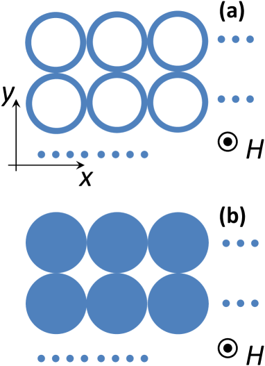
Figure 1: (Color online) Schematic top-view of two-dimensional patterned magnetic thin films (blue region represents magnetic media, while the other stands for the vacuum). An external magnetic field is applied perpendicular to the plane with out-of-plane moments. Either circular rings (a) or disks (b) form a square lattice. We assume that the film is sufficiently thin, so that there is no texture along the direction perpendicular to the plane.

II ring model

To begin with, consider spin-wave excitations in a magnetic circular ring. When a linear dimension of a cross section of the ring is comparable to short-ranged exchange length $l_{\rm ex}$ of a constituent magnetic material, the ring may be treated as a one-dimensional chain of $M$ spins, which are coupled with one another via long-range dipole-dipole interaction. $M$ is the number of the spins along the ring and is on the order of $2\pi r/l_{\rm ex}$ ($r$ is the radius of the ring). Without the field, the magnetostatic energy is minimized by a vortex spin configuration: spins are aligned along the tangential direction of the ring. Under the out-of-plane magnetic field $H$, the vortex spin configuration acquires an out-of-plane moment which becomes fully polarized above the saturation field, $H>H_{c}$.

Suppose that the amplitude of each spin moment is fixed to be $M_{s}$. Excitations in each spin comprise two real-valued fields (transverse moments), so that the ring has $M$ numbers of complex-valued spin-wave modes, $\psi(\theta_{j})$ with $\theta_{j}\equiv 2\pi j/M$ ($j=1,\cdots,M$). Under a proper gauge choice (see appendix A), they have total angular momentum $q_{J}$ as their quantum number,

$$\psi_{q_{J}}(\theta_{j}+\theta_{m})=e^{iq_{J}m}\psi_{q_{J}}(\theta_{j}),$$ (1)

which comes from the circular rotational symmetry of a ring. Here $\theta_{j}\equiv 2\pi j/M$ and $q_{J}\equiv 2\pi n_{J}/M$ $(n_{J}=-M/2,-M/2+1,\cdots,M/2)$. The resonance frequency for these ‘atomic orbitals’ is given as a function of the angular momentum, which forms a frequency band for larger $M$.

At the zero field, all the spins in the circular vortex is along the angular momentum axis (along the tangential direction of the ring), so that the frequency band at $H=0$ becomes essentially same as the ‘backward’ volume modes in an in-plane magnetized thin film DV2 ; Kalinikos or cylindrically magnetized nanowire. AM Namely, the band has its resonance frequency minimum at $q_{J}=\pi$ and its frequency maximum at $q_{J}=0$. When increasing the out-of-plane field, the maximum and minimum are inverted at some ‘critical’ field below the saturation field, $H=H_{d}\simeq 0.8H_{c}$ (Fig. 2 (a,b)). The resonance frequency mode at $q_{J}=0$ becomes eventually gapless at $H=H_{c}$, being consistent with the classical spin configuration which starts to acquire finite in-plane components forming a circular vortex for $H<H_{c}$. For $H>H_{c}$, these excitations become gapped again with the minimum being at $q_{J}=0$. For $H\gg H_{c}$, a ‘band center’ of these resonance frequency levels converges to usual ferromagnetic resonance (FMR) mode. Note also that two time-reversal-pair modes, $q_{J}$ and $-q_{J}$, are degenerate at the zero field, while they are not under a finite field. For the out-of-plane field along $+z$ direction, $\varepsilon_{q_{J}}<\varepsilon_{-q_{J}}$ for $q_{J}\gtrsim 0$ (see Fig. 2(b,c,d)).

When a circular ring embedded into the square lattice, the quantum number for the atomic orbital reduces to either one of the following four, $q_{J}=0,\pm\frac{2\pi}{M},\frac{4\pi}{M}$. Namely, each ring feels an anisotropic demagnetization field from its surrounding rings, which respects four-fold rotational symmetry. This mixes any two states whose $q_{J}$ differs by $\frac{8\pi}{M}$ (Fig. 2 (c,d)). Under the four-fold rotation, these four atomic orbital wave functions acquire $+1$, $\pm i$ and $-1$, which suggests that they are essentially $s$-wave, $p_{\pm}=p_{x}\pm ip_{y}$-wave and $d_{x^{2}-y^{2}}$-wave function respectively;

$$\psi^{(n)}_{s}\big{(}\theta_{j}+\frac{\pi}{2}\big{)} =\psi^{(n)}_{s}\big{(}\theta_{j}\big{)},$$ (2)

$$\psi^{(n)}_{p_{\pm}}\big{(}\theta_{j}+\frac{\pi}{2}\big{)} =\pm i\!\ \psi^{(n)}_{p_{\pm}}\big{(}\theta_{j}\big{)},$$ (3)

$$\psi^{(n)}_{d_{x^{2}-y^{2}}}\big{(}\theta_{j}+\frac{\pi}{2}\big{)} =-\psi^{(n)}_{d_{x^{2}-y^{2}}}\big{(}\theta_{j}\big{)}.$$ (4)

Every fourth levels from below are grouped together in the frequency space, forming a branch specified by the superscript index $n$ (Fig. 2(d)); every branch includes the four types of wave functions, $s$, $p_{\pm}$, $d_{x^{2}-y^{2}}$-wave functions. The corresponding atomic orbital levels are arranged in the frequency space as

$$\varepsilon^{(1)}_{s}<\varepsilon^{(1)}_{p_{+}}<\varepsilon^{(1)}_{p_{-}}<\varepsilon^{(1)}_{d_{x^{2}-y^{2}}}<$$

$$\ \ \varepsilon^{(2)}_{d_{x^{2}-y^{2}}}<\varepsilon^{(2)}_{p_{-}}<\varepsilon^{(2)}_{p_{+}}<\varepsilon^{(2)}_{s}<\varepsilon^{(3)}_{s}<\varepsilon^{(3)}_{p_{+}}<\cdots.$$ (5)

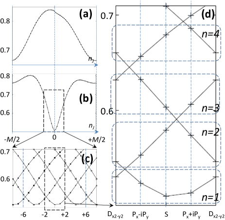
Figure 2: (Color online) Resonance frequency levels in a magnetic ring (a $M$-spins chain with $M=60$) as a function of the angular momentum $q_{J}\equiv\frac{2\pi n_{J}}{M}$ with $n_{J}=-M/2,-M/2+1,\cdots,M/2$. (a) $H=0.7H_{c}$ and (b) $H=0.9H_{c}$. (c) When demagnetization fields from the surrounding magnetic rings are included, the angular momentum $n_{J}$ is defined mod $4$. (d) Wave functions with $n_{J}\equiv$ $-1$,$0$,$+1$, $+2$ (mod $4$) are referred to as $P_{-}$,$S$,$P_{+}$ $D_{x^{2}-y^{2}}$-wave respectively, since they acquire $-i$, $+1$, $+i$ and $-1$ phase under the $\frac{\pi}{2}$ spatial rotation (eqs. (2,3,4)).

When inter-ring ‘exchange’ processes via magnetic dipole-dipole interaction are included, these atomic orbitals constitute extended volume-mode bands. When neighboring branches are sufficiently separated from each other by the anisotropic demagnetization field, the volume-mode bands can be constructed out of each branch separately;

$$\big{\{}\psi^{(2m+1)}_{s},\psi^{(2m+1)}_{p_{+}},\psi^{(2m+1)}_{p_{-}},\psi^{(2m+1)}_{d_{x^{2}-y^{2}}}\big{\}},$$ (6)

or

$$\big{\{}\psi^{(2m+2)}_{d_{x^{2}-y^{2}}},\psi^{(2m+2)}_{p_{-}},\psi^{(2m+2)}_{p_{+}},\psi^{(2m+2)}_{s}\big{\}}.$$ (7)

Each branch provides four volume-mode bands. A qualitative feature of the four volume-mode bands can be roughly captured by a two-orbital model made out of the lower two atomic orbital wave functions within each branch;

$$\big{\{}\psi^{(2m+1)}_{s},\psi^{(2m+1)}_{p_{+}}\big{\}},\ \ {\rm or}\ \ \big{\{}\psi^{(2m+2)}_{d_{x^{2}-y^{2}}},\psi^{(2m+2)}_{p_{-}}\big{\}}.$$ (8)

This is because lower two atomic orbitals within each branch have less nodes than the other two along the ring. The inter-ring transfer integrals among such two are expected to be larger than those otherwise.

From the symmetry point of view, a nearest neighbor tight-binding model composed of the lower two orbitals is given by;

$$\hat{H}_{01} =\sum_{\bm{b}}\big{(}\varepsilon_{0}\gamma^{\dagger}_{0,{\bm{b}}}\gamma_{0,{\bm{b}}}+\varepsilon_{1}\gamma^{\dagger}_{1,{\bm{b}}}\gamma_{1,{\bm{b}}}\big{)}$$

$$-\sum_{\bm{b}}\sum_{\mu=x,y}\sum_{\sigma=\pm}\big{(}a_{00}\gamma^{\dagger}_{0,{\bm{b}}}\gamma_{0,{\bm{b}}+\sigma{\bm{e}}_{\mu}}-a_{11}\gamma^{\dagger}_{1,{\bm{b}}}\gamma_{1,{\bm{b}}+\sigma{\bm{e}}_{\mu}}\big{)}$$

$$\hskip 14.22636pt-\sum_{\bm{b}}\sum_{\sigma=\pm}\big{(}-\sigma b_{01}\gamma^{\dagger}_{0,{\bm{b}}}\gamma_{1,{\bm{b}}+\sigma{\bm{e}}_{x}}+{\rm H.c.}\big{)}$$

$$\hskip 14.22636pt-\sum_{\bm{b}}\sum_{\sigma=\pm}\big{(}-i\sigma b_{01}\gamma^{\dagger}_{0,{\bm{b}}}\gamma_{1,{\bm{b}}+\sigma{\bm{e}}_{y}}+{\rm H.c.}\big{)}.$$ (9)

Here $\gamma^{\dagger}_{0,{\bm{b}}}$ ($\gamma_{0,{\bm{b}}}$) and $\gamma^{\dagger}_{1,{\bm{b}}}$ ($\gamma_{1,{\bm{b}}}$) stand for creation (annihilation) operators for parity-even and parity-odd atomic orbitals respectively. The subscript ${\bm{b}}$ denotes a coordinate of a center of a ring which the orbitals belong to. ${\bm{e}}_{\mu}$ is the primitive translation vector of the square lattice ($\mu=x,y$). The parity-even atomic orbital refers to $s$-wave or $d_{x^{2}-y^{2}}$-wave, while the parity-odd atomic orbital refers to $p_{\pm}$-wave:

$$\big{\{}\varepsilon_{0},\varepsilon_{1}\big{\}}=\big{\{}\varepsilon^{(2m+1)}_{s},\varepsilon^{(2m+1)}_{p_{+}}\big{\}},\ \ {\rm or}\ \big{\{}\varepsilon^{(2m+2)}_{d_{x^{2}-y^{2}}},\varepsilon^{(2m+2)}_{p_{-}}\big{\}},$$

so that $\varepsilon_{0}<\varepsilon_{1}$. A general observation of orbital shapes suggests that $a_{00}$, $a_{11}$ and $b_{01}$ are all positive real values under a proper gauge choice.

The tight binding Hamiltonian in the momentum space is expanded in term of the Pauli matrices as, $H({\bm{k}})=c({\bm{k}})\!\ {\bm{\sigma}}_{0}+\sum^{3}_{j=1}{\bm{h}}_{j}({\bm{k}})\!\ {\bm{\sigma}}_{j}$ with $h_{3}({\bm{k}})\equiv\epsilon_{0}-\epsilon_{1}-2(a_{00}+a_{11})(\cos k_{x}+\cos k_{y})$, $h_{1}({\bm{k}})\equiv 2b_{01}\sin k_{y}$ and $h_{2}({\bm{k}})\equiv 2b_{01}\sin k_{x}$. In terms of a vector field ${\bm{h}}({\bm{k}})$, the topological Chern integer for the two volume-mode bands obtained from this Hamiltonian can be defined as a wrapping number of a normalized vector $\overline{\bm{h}}({\bm{k}})\equiv{\bm{h}}({\bm{k}})/|{\bm{h}}({\bm{k}})|$. Volovik ; Yakovenko ; QWZ The integer counts how many times the normalized vector wraps the unit sphere, when the momentum ${\bm{k}}$ wraps around the two-dimensional Brillouin zone with the torus geometry; Volovik ; Yakovenko ; QWZ

$$c_{+}=-c_{-}=\int_{[-\pi,\pi]^{2}}\frac{d^{2}{\bm{k}}}{4\pi}\!\ \!\ \overline{\bm{h}}({\bm{k}})\cdot\big{(}\partial_{k_{x}}\overline{\bm{h}}({\bm{k}})\times\partial_{k_{y}}\overline{\bm{h}}({\bm{k}})\big{)}.$$

Within a two-band model, the integer for the upper band ($c_{+}$) always has an opposite sign to that for the lower band ($c_{-}$). When two nearest neighboring rings are spatially proximate to each other, larger exchange integrals realize $\varepsilon_{1}-\varepsilon_{0}<4(a_{00}+a_{11})$, which makes the wrapping number to be unit. Namely, the unit vector points at the south pole/north pole ($\bar{\bm{h}}=(0,0,-1)$/$(0,0,+1)$) at ${\bm{k}}=(0,0)$/$(\pi,\pi)$, while the vector winds once around the south pole/north pole when ${\bm{k}}$ rotates once around the ${\bm{k}}=(0,0)$/$(\pi,\pi)$. This observation suggests that the Chern integers for two bands obtained from eq. (9) become $\{c_{-},c_{+}\}=\{-1,+1\}$. When the out-of-field direction is reversed, $p_{+}$ and $p_{-}$ are exchanged in

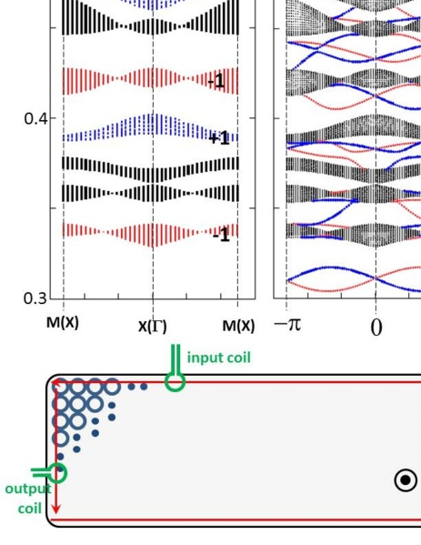
Figure 3: (Color online) Wavelength-frequency dispersions for spin-wave excitations for $H_{d}<H<H_{c}$ $(H=0.94H_{c})$. (a) A side-view of lowest 8 volume-mode bands with the Chern integer. The red bands have $-1$ Chern integer, while blue bands have $+1$. The dispersions are calculated with periodic boundary conditions for both $x$ and $y$-directions. Since the 7th and 8th lowest band have frequency degeneracies around $M$-points, only the sum of their integers is quantized to $+1$. (b) Spin-wave excitations calculated with an open/periodic boundary condition along the $y$/$x$-direction respectively. The resonance frequencies are given as a function of the wave vector along the $x$-direction. The system along the $y$-direction includes 18 square-lattice unit cells ($L=18$). More than $75\%$ of amplitudes of eigen wave functions with red points are localized within $y=1$ and $y=2$, while those with blue points are localized within $y=L-1$ and $y=L$ (edge modes). Compared with Fig. (a), the calculated spectra have additional spin-wave modes which are localized along the edges. (c) With the out-of-plane field up-headed, the chiral edge modes rotate in the counterclockwise way.

Fig. 2(d) and eqs. (6,7), which changes the sign of the last term in eq. (9) and that of $c_{\pm}$. Note also that, to have the non-zero wrapping number, it is essential that ‘wave function character’ for the lower/higher band at ${\bm{k}}=(\pi,\pi)$ is parity odd/even atomic orbital, while that at the ${\bm{k}}=(0,0)$ is parity-even/odd one (‘band inversion’). BTZ ; FK When $\varepsilon_{1}-\epsilon_{0}>4(a_{00}+a_{11})$, wave function character of the lower (higher) band at ${\bm{k}}=(\pi,\pi)$ and that of ${\bm{k}}=(0,0)$ have same parity, so that the unit vector always stays within the southern hemisphere, irrespective of the momentum ${\bm{k}}$; the wrapping number always reduces to zero.

The argument so far suggests that, in the presence of larger inter-ring transfer integrals, the distribution of the Chern integers for soft volume-mode bands at $H_{d}<H<H_{c}$ can be non-trivial and is composed of a sequence of $\{-1,+1,0,0\}$ from below;

$$\big{\{}c_{1},c_{2},c_{3},c_{4}\!\ \big{|},c_{5},c_{6},c_{7},c_{8}\!\ \big{|},\cdots\big{\}}$$

$$\ \ =\big{\{}-1,+1,0,0\!\ \big{|},-1,+1,0,0\!\ \big{|},\cdots\big{\}}$$ (10)

where $c_{n}$ denotes the integer for the $n$-th lowest band (see also appendix A for general definition of the topological Chern integer for volume-mode spin-wave bands). An explicit calculation of the Chern integers for volume-mode bands within $H_{d}<H<H_{c}$ based on a linearized Landau-Lifshitz equation confirms this feature with a minor modification. In the actual calculation, we also observed that, within each branch, another band inversion is often induced by relatively stronger exchange integrals between higher two atomic orbitals and the 2nd lowest atomic orbital, which transfer the non-zero integer of the 2nd lowest band into the 3rd or 4th lowest bands in each branch, $\{-1,+1,0,0\}\rightarrow\{-1,0,+1,0\}$ or $\{-1,0,0,+1\}$. Which comes true among these three, i.e. $\{-1,+1,0,0\}$, $\{-1,0,+1,0\}$ and $\{-1,0,0,+1\}$, depends on specific branch and other details, while the integer for the lowest band ($-1$) remains intact in every branch ,e.g.

$$\big{\{}c_{1},c_{2},c_{3},c_{4}\!\ \big{|},c_{5},c_{6},c_{7},c_{8}\!\ \big{|},\cdots\big{\}}$$

$$\ \ =\big{\{}-1,0,0,+1\!\ \big{|},-1,0,\alpha,1-\alpha\!\ \big{|},\cdots\big{\}},$$ (11)

(Fig. 3(a)).

General arguments SO1 ; SO2 based on a bulk-edge correspondence in IQH physics TKKN ; Hal ; Hat dictate that the Chern integers for the volume-mode bands shown in eq. (11) lead to counterclockwise rotating spin-wave edge modes, whose chiral dispersion connects in the frequency space a volume-mode band with $-1$ Chern integer and that with $+1$ Chern integer. In fact, the existence of such chiral edge modes are confirmed by quantitative band calculations based on a linearized Landau-Lifshitz equation with open boundary condition (Fig. 3(b)). Again, reversing the out-of-field direction ($+z\rightarrow-z$) results in the sign change of $c_{n}$, which changes the chiral direction of the edge modes from counterclockwise to clockwise (Fig. 3(c)).

When the out-of-plane field is less than the ‘critical’ field, $H<H_{d}$, the lower spin-wave volume mode bands are from those atomic orbitals having higher total angular momentum $q_{J}=\pi$. Compared to those around $q_{J}=0$, such orbitals have many nodes along the ring; their wave functions change sign under the translation only by one spin, e.g.

$$\psi_{q_{J}=\pi}(\theta_{j+1})=-\psi_{q_{J}=\pi}(\theta_{j}).$$

Due to this many-node structure, transfer integrals between the higher angular momentum orbitals ($q_{J}\simeq\pi$) become much smaller than those between orbitals with lower angular momentum ($q_{J}\simeq 0$). As a result, low-frequency volume-mode bands for $H<H_{d}$ have tiny dispersions, which can hardly fulfill the band inversion condition, $|\epsilon_{1}-\epsilon_{0}|<4(a_{00}+a_{11})$; we thus cannot expect the chiral spin-wave edge modes.

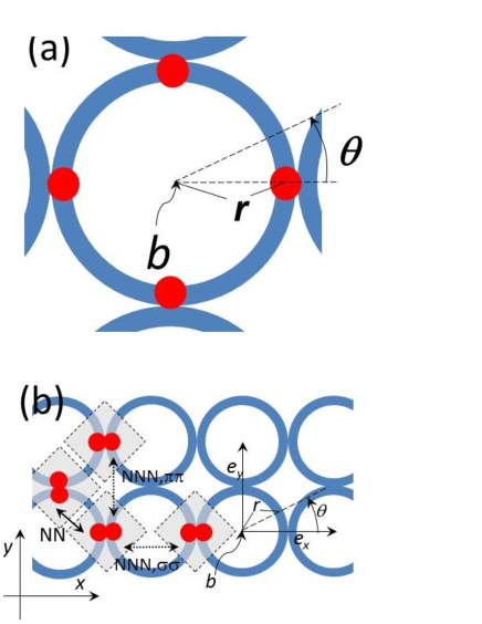
Figure 4: (Color online) (a) Four corners in a ring (red regions; $\theta=0,\frac{\pi}{2},\pi,\frac{3\pi}{2}$) feel larger demagnetization field than other regions. ${\bm{b}}$ denotes a coordinate of the center of the ring, while $r$ is a radius of the ring. (b) two-orbital tight-binding model with nearest-neighbor (‘NN’ in the figure) inter-cluster transfer integral (${\bm{H}}_{0}$), next-nearest-neighbor $\sigma$-$\sigma$ coupling (‘NNN,$\sigma\sigma$’) inter-cluster transfer integral (${\bm{H}}_{1}$ with $c$) and next-nearest-neighbor $\pi$-$\pi$ coupling (‘NNN,$\pi\pi$’) inter-cluster transfer integral (${\bm{H}}_{1}$ with $c^{\prime}$). The in-phase orbital (red peanut-shape item) at the $x$-link is extended along the $x$-direction, while that at the $y$-link is along the $y$-direction. ${\bm{e}}_{x}$ and ${\bm{e}}_{y}$ denote the primitive translation vectors of the square lattice.

Above the saturation field ($H>H_{c}$), the four-fold rotational anisotropy in the demagnetization field becomes stronger. When the classical spin configuration becomes fully polarized along the out-of-plane field, spins in a ring which are proximate to its four nearest neighboring rings especially feel stronger demagnetization fields than those spins in the ring which are not. In terms of the angle variable $\theta$ defined as ${\bm{r}}\equiv{\bm{b}}+r(\cos\theta,\sin\theta)$ (${\bm{b}}$ denotes a coordinate of a center of the ring at which a spin at ${\bm{r}}$ is included and $r$ is the radius of the ring; see fig. 4(a)), these spins are at the four corners of a ring, $\theta=0,\frac{\pi}{2},\pi,\frac{3\pi}{2}$ respectively. As a result of this strongly anisotropic demagnetization field, soft spin-wave excitations for $H>H_{c}$ are highly localized around these four corners.

From this point of view, we made another tight binding model for soft spin-wave bands, which is valid only above the saturation field (appendix B). Thereby, we first took into account proximate ‘exchange process’ which transfers a spin in a corner of a ring into its closest corner of the nearest neighboring ring. The inclusion of such exchange process leads to in-phase and out-of-phase orbital wave functions formed by these two spins. These ‘atomic-orbital’ wave functions are on a center of a link connecting two nearest neighboring rings (red peanut-shape items in Fig. 4(b)). It turns out that, when the field is not too close to the saturation field, the in-phase atomic orbital level becomes lower than the out-of-phase orbital level (see Appendix B for the argument).

The square lattice has two inequivalent links within its unit cell, the link along the $x$-axis (‘$x$-link’) and that along the $y$-axis (‘$y$-link’). Each link provides in-phase and out-of-phase orbital wave functions. Since the out-of-phase wave function has a node at the center, while the in-phase one does not, inter-link transfer integrals between out-of-phase orbitals becomes smaller than those between in-phase orbitals. Being interested in spin-wave bands with larger band width, we focus only on the in-phase orbital wave functions.

A transfer integral between $x$-link and its nearest neighbor $y$-link becomes complex-valued;

$$H_{0} =\sum_{{\bm{b}}}\Big{\{}(ia+b)\!\ \beta^{\dagger}_{{\bm{b}}+\frac{{\bm{e}}_{y}}{2}}\beta_{{\bm{b}}+\frac{{\bm{e}}_{x}}{2}}$$

$$\ \ \ -(ia+b)\!\ \beta^{\dagger}_{{\bm{b}}+{\bm{e}}_{y}+\frac{{\bm{e}}_{x}}{2}}\beta_{{\bm{b}}+\frac{{\bm{e}}_{y}}{2}}$$

$$\ \ \ \ +(ia+b)\!\ \beta^{\dagger}_{{\bm{b}}+{\bm{e}}_{x}+\frac{{\bm{e}}_{y}}{2}}\beta_{{\bm{b}}+{\bm{e}}_{y}+\frac{{\bm{e}}_{x}}{2}}$$

$$\ \ \ \ \ \ -(ia+b)\!\ \beta^{\dagger}_{{\bm{b}}+\frac{{\bm{e}}_{x}}{2}}\beta_{{\bm{b}}+{\bm{e}}_{x}+\frac{{\bm{e}}_{y}}{2}}+{\rm h.c.}\Big{\}}$$ (12)

with real-valued $a$ and $b$. $\beta_{{\bm{b}}+\frac{{\bm{e}}_{x}}{2}}$ and $\beta_{{\bm{b}}+\frac{{\bm{e}}_{y}}{2}}$ represent annihilation operators for the in-phase orbital on the $x$-link (whose center is at ${\bm{b}}+\frac{{\bm{e}}_{x}}{2}$) and that on $y$-link (at ${\bm{b}}+\frac{{\bm{e}}_{y}}{2}$) respectively. ‘$ia\equiv ae^{i\theta}$’ with $\theta=\frac{\pi}{2}$ in eq. (12) comes from 90^∘ degree angle subtended by the two nearest neighbor orbitals at ${\bm{b}}+\frac{{\bm{e}}_{x}}{2}$ and at ${\bm{b}}+\frac{{\bm{e}}_{y}}{2}$ and a center of the ring at ${\bm{b}}$. ‘$b$’ in eq. (12) results from a finite particle-hole mixing (see appendix B for the derivation of eq. (12)). A band structure obtained from $H_{0}$ has two frequency bands which form gapless Dirac cone spectra at ${\bm{k}}=(\pi,0)$ and $(0,\pi)$.

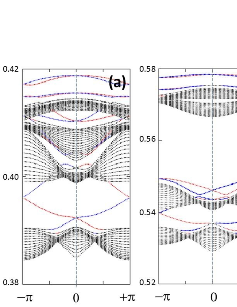
Figure 5: (Color online) Wavelength-frequency dispersions for lowest four volume-mode bands and chiral edge modes in $H>H_{c}$ (a) $H=1.09H_{c}$ (b) $H=1.17H_{c}$. The dispersion are obtained with an open/periodic boundary condition along the $y$/$x$-direction, where the resonance frequencies for spin wave excitations are given as a function of the wave vector along the $x$-direction. We used the same system size along the $y$-direction as in Fig. 3 and the same definition of red and blue points as in Fig. 3. In both (a) and (b), the lowest two volume modes (black points) consist of the in-phase atomic orbitals on $x$-link and $y$-link, while the upper two volume modes mainly consist of out-of-phase orbitals on these two links. The spectra clearly contain a chiral edge mode connecting the lowest two volume-mode bands. Compared to the lowest two bands, the 3rd and 4th lowest bands have smaller band width and no band gap in between. This is because, contrary to the in-phase atomic orbital, the out-of-phase atomic orbital has a node at the center of each link, which results in smaller transfer integrals. Compared (a) and (b), note also that a frequency spacing between the in-phase atomic orbital level and the out-of-phase atomic orbital level increases on increasing the field (see appendix B for the reasoning).

A finite transfer between the nearest $x$-links and that between the nearest $y$-links endows the gapless Dirac cone spectra with a finite mass. The transfer takes a form of,

$$H_{1} =\sum_{{\bm{b}}}\Big{\{}c\!\ \beta^{\dagger}_{{\bm{b}}+\frac{{\bm{e}}_{x}}{2}}\beta_{{\bm{b}}-\frac{{\bm{e}}_{x}}{2}}+c\!\ \beta^{\dagger}_{{\bm{b}}+\frac{{\bm{e}}_{y}}{2}}\beta_{{\bm{b}}-\frac{{\bm{e}}_{y}}{2}}$$

$$\ \ \ +c^{\prime}\!\ \beta^{\dagger}_{{\bm{b}}+{\bm{e}}_{y}+\frac{{\bm{e}}_{x}}{2}}\beta_{{\bm{b}}+\frac{{\bm{e}}_{x}}{2}}+c^{\prime}\!\ \beta^{\dagger}_{{\bm{b}}+{\bm{e}}_{x}+\frac{{\bm{e}}_{y}}{2}}\beta_{{\bm{b}}+\frac{{\bm{e}}_{y}}{2}}+{\rm h.c.}\Big{\}},$$ (13)

with real-valued $c$ and $c^{\prime}$. Now that orbital wave function at the $\mu$-link is extended along the $\mu$-axis, ‘$c$’ stands for the ($\sigma,\sigma$)-coupling next nearest neighbor (NNN) transfer integral, while ‘$c^{\prime}$’ stands for the $(\pi,\pi)$-coupling NNN transfer integral (Fig. 4(b)). Amplitudes of transfer integrals are inversely proportional to the cubic in distance, so that $|c|>|c^{\prime}|$. A finite $|c-c^{\prime}|$ induces a gap in the gapless Dirac cone spectra.

The Chern integers for these two spin-wave bands can be evaluated from the wrapping number of the normalized vector $\overline{\bm{h}}({\bm{k}})\equiv{\bm{h}}({\bm{k}})/|{\bm{h}}({\bm{k}})|$. For eqs. (12,13), $h_{1}({\bm{k}})=4b\sin\frac{k_{x}}{2}\sin\frac{k_{y}}{2}$, $h_{2}({\bm{k}})=4a\cos\frac{k_{x}}{2}\cos\frac{k_{y}}{2}$ and $h_{3}({\bm{k}})=2(c-c^{\prime})(\cos k_{x}-\cos k_{y})$. When the momentum rotates around ${\bm{k}}=(\pi,0)$ / $(0,\pi)$, $\overline{\bm{h}}({\bm{k}})$ rotates around the south pole/ north pole once for $c>c^{\prime}$; the winding numbers are $\pm 1$. More generally, the integers for these two bands are $\{c_{-},c_{+}\}=\{+1,-1\}$ from below for $(c-c^{\prime})\cdot a\cdot b>0$, while $\{-1,+1\}$ for $(c-c^{\prime})\cdot a\cdot b<0$. In either case, there appears a chiral edge mode within the band gap, whose sense of rotation along the boundary is clockwise for the former case, while counterclockwise for the latter case. A primitive evaluation suggests that $a>0$, $b>0$ and $c<c^{\prime}<0$ (appendix B), so that a counterclockwise chiral edge mode is expected. In fact, the counterclockwise chiral edge mode is observed within a band gap between the lowest and the 2nd lowest volume-mode band for a wide field range of $H>H_{c}$ (Fig. 5). Contrary to the effective $s$-$p_{\pm}$ model for $H_{d}<H<H_{c}$, the band gap and the chiral edge mode in the present two-orbital model persist for a wider range of $H>H_{c}$. This is because any symmetries in the model requires neither $c=c^{\prime}$ nor $a=0$, while $b$ vanishes only in the large $H$ limit (appendix B). This feature is indeed justified by the micromagnetic simulation in sec. IV.

III disk model

Let us next consider spin-wave excitations in circular disk model. We simulate the magnetic disk by a cluster of many spins, each of which has a same volume element. The spins are distributed as homogeneously in space as possible (see the caption of Fig. 6). Physically, a linear dimension of the volume element should be on the order of short-ranged exchange interaction length $l_{\rm ex}$. The spins are coupled with one another via magnetic dipole-dipole interaction.

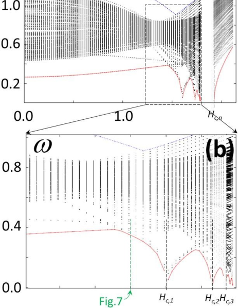
Figure 6: (Color online) (a,b) Distribution of resonance frequency levels of magnon modes in a single circular magnetic disk as a function of the out-of-plane field. The four-fold-rotational demagnetization field from other disks are also included in the calculation. The red curve plots the lowest resonance frequency level as a function of the out-of-plane field, while the blue curve represents the highest resonance frequency level. We simulate the circular magnetic disk by a cluster of spins, respecting the circular symmetry as much as possible. For a given radius $R$, we discretize $R$ into $n$ pieces. For the radial coordinate ranging from $[\frac{Rj}{n},\frac{R(j+1)}{n}]$ ($j=0,1,\cdots,n-1$), we discretize the azimuth coordinate into $4(2j+1)$ pieces, so that area of each element is same, $\frac{\pi R^{2}}{4n^{2}}$. We put a spin at the center of each element specified by $(x,y)=r_{j}(\cos\theta_{j,m},\sin\theta_{j,m})$ with $r_{j}=\frac{R(2j+1)}{2n}$ and $\theta_{j,m}=\frac{\pi(2m+1)}{4(2j+1)}$ ($m=0,\cdots,4(2j-1)$). In the calculation, we take $n=8$, so that a cluster has $256$ spins.

A circular vortex structure minimizes the magnetostatic energy of the disk at the zero field, while the field induces a finite out-of-plane magnetization. Suppose that spins are nearly polarized along the field, while any of them are not yet fully polarized. Being surrounded by many others, spins around the center of a disk feel the strongest demagnetization field, while the demagnetization field around the boundary is smallest. Thus, spins at the boundary become fully polarized first by a relatively lower field, $H_{c,1}$, while spins around the center become fully polarized at last by a relatively higher field, $H_{c,n}(>H_{c,1})$. In the present discrete spin model, these two critical fields encompasses a couple of other critical fields ($H_{c,1}<H_{c,2}<H_{c,3}<\cdots<H_{c,n}$), at which interior spins get fully polarized successively from the outer to the inner on increasing the field.

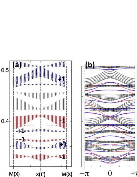
Figure 7: (Color online) Wavelength-frequency dispersions for spin-wave excitations for $H<H_{c,1}$ (see Fig. 6(b)) (a) wavelength-frequency dispersion for volume-mode bands with the Chern integer ($H=0.94H_{c,1})$. The dispersions are calculated with periodic boundary conditions for both $x$ and $y$-directions. (b) wavelength-frequency dispersion for volume-mode bands and edge-mode bands ($H=0.94H_{c,1}$) calculated with an open/periodic boundary condition along the $y$/$x$-direction. Resonance frequencies are given as a function of the wave vector along the $x$-direction. The system along the $y$-direction includes 9 unit cells ($L=9$). More than $50\%$ of amplitudes of eigen wave functions with red points are localized only within $y=1$, while those for blue points are localized from $y=L$ (edge modes). Compared with Fig. (a), the spectra have additional spin-wave modes which are localized along the edges, whose chiral dispersion connect spin-wave volume modes bands with opposite Chern integers

Correspondingly, spin wave excitations, which are fully gapped at $H=0$, become gapless or significantly softened at each of these critical fields, $H=H_{c,1},H_{c,2},\cdots$ (Fig. 6). Especially, the soft magnons around $H=H_{c,1}$ are localized around the boundary of the disk, while those around $H=H_{c,n}$ are localized at the center. In a single magnetic disk, spin-wave excitations have the total angular momentum $q_{J}$ as a good quantum number. All the soft magnons around these critical fields come from $q_{J}=0$, so as to be consistent with the classical spin configuration. In the presence of the four-fold rotational demagnetization field, these soft magnons take a form of either $s$-wave ($n_{J}=0$), $p_{\pm}$-wave ($n_{J}=\pm 1$) or $d_{x^{2}-y^{2}}$-wave ($n_{J}=2$) atomic orbital. As in the ring model, an inter-disk exchange process via the dipolar interaction makes these atomic orbitals to form extended volume-mode bands.

Since the soft magnons around $H=H_{c,1}$ are localized around the boundary of the disk, the inter-disk transfer integrals between these magnons become larger and soft volume-mode bands around $H=H_{c,1}$ become similar to what we observed in the ring model at $H\simeq H_{c}$; the distribution of Chern integers for a set of these four bands becomes either $\{-1,+1,0,0\}$, $\{-1,0,+1,0\}$, or $\{-1,0,0,+1\}$ from below (Fig. 7(a)). Again, this leads to a counterclockwise chiral edge mode between these two (Fig. 7(b)).

On the other hand, the soft magnons in $H\gtrsim H_{c,n}$ are localized around the center of the disk, so that the inter-disk transfer integrals between these atomic orbitals are very small. As a result, soft volume-mode bands in $H\gtrsim H_{c,n}$ have tiny dispersions, where we cannot expect any band inversion mechanism.

IV micromagnetic simulation

In order to uphold the existence of the chiral edge mode in the proposed magnetic superlattices, we perform a micromagnetic simulation by solving the Landau-Lifshitz-Gilbert equation in terms of the 4th order Runge-Kutta method with a unit time step 1ps. Fig. 8 shows an entire magnetic superlattice, which contains 14 $\times$ 14 unit cells with open boundaries. Each unit cell contains 12 ferromagnetic grains, forming a square-shape ring. Each grain is 5-nanometer cube. Note also that, not including any short-range exchange interaction (see below), the following result is scalable; provided that each ferromagnetic grain behaves as single spin, the size of the grain can be much larger than 5-nanometer and the scale of resonance frequency and saturation field still remain unaltered. The saturation magnetization and Gilbert damping coefficient of the ferromagnetic grain are set to 135300 A/m and 1.0$\times$10^-5 respectively. We regard each nanograin as a uniform magnet, assigning single spin degree of freedom to each grain. Different ferromagnetic nanograins are coupled with one another through the magnetic dipole-dipole interaction. Under a static out-of-plane field (along the $z$ direction) greater than 620 Oe, a stable spin configuration becomes fully polarized along the field, while the configuration acquires finite in-plane components below 620 Oe. We studied spin-wave excitations above the saturation field ($\gtrsim$ 620 Oe).

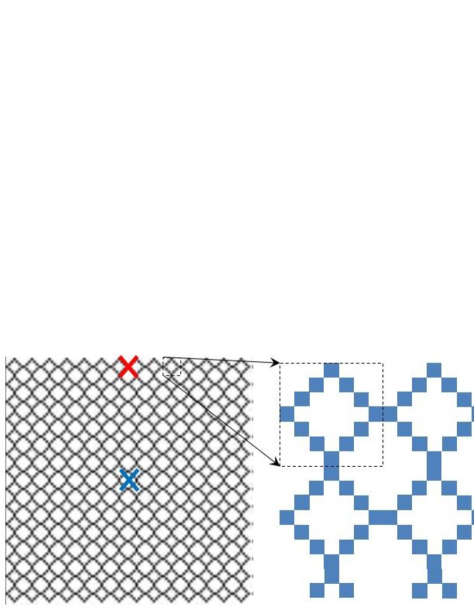
Figure 8: (Color online) magnetic superlattice with 14 $\times$ 14 unit cell. (right) a unit cell contains 12 ferromagnetic grain forming a square ring. Each grain is cubic-shape with its linear dimension $5$ nm. (left) To excite volume-mode/edge-mode excitations, we apply a pulse field at the center/boundary of the superlattice (blue/red crossed point) respectively.

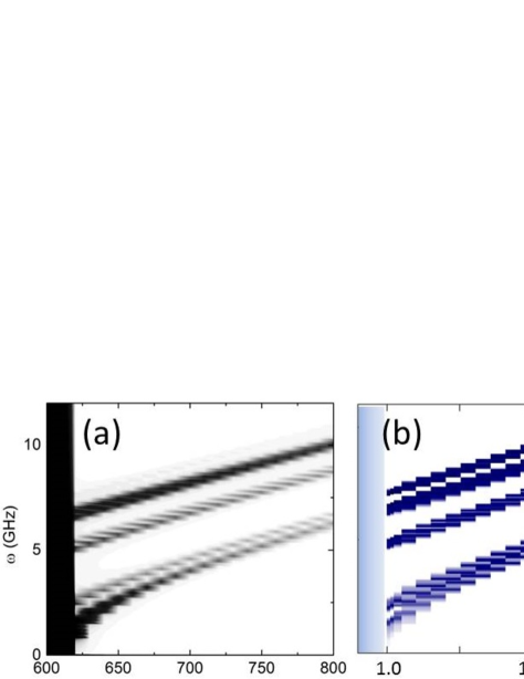
Figure 9: (Color online) (a) Contour plot of the integrated power specctrum $A(\omega)$ as a function of the static out-of-plane field $H$, where the initial pulse field is applied at the center of the magnetic superlattice. The out-of-plane field is greater than the saturation field ($\simeq$ 620 Oe). (b) Contour plot of the density of state for volume-mode bands obtained from spin-wave calculations on the same magnetic superlattice. The horizontal axis is the static out-of-plane field, where the unit is taken to be the saturation field. In both figures, darker regions have higher intensities.

To study spin wave modes in a broad frequency range at once, we apply a pulse magnetic field in a transverse ($x$) direction (pulse time $1$ ps and amplitude $1$ Oe). We then calculate a time evolution of magnetization dynamics afterward, and take a Fourier transformation of the transverse moments with respect to time;

$$s_{+}(X,Y,\omega)\equiv\sum_{j=0}^{n-1}m_{+}(X,Y,j\Delta T)\exp\left(2\pi{\rm i}\omega j\Delta T\right)$$ (14)

with $m_{+}(X,Y,t)\equiv m_{x}(X,Y,t)+{\rm i}m_{y}(X,Y,t)$, $\Delta T=100$ ps and $n=1024$. An amplitude of the frequency power spectrum, $|s_{+}(X,Y,\omega)|$, represents a sort of local density of state of spin-wave modes at the resonance frequency $\omega$. When integrated over the two-dimensional space coordinates, ($X,Y$), the power spectrum represents the total density of states at $\omega$;

$$A(\omega)\equiv\sum_{X,Y}\big{|}s_{+}(X,Y,\omega)\big{|},$$ (15)

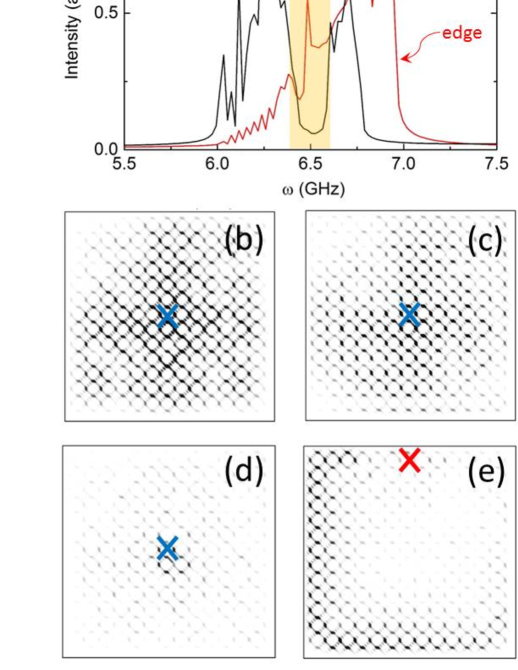
Figure 10: (Color online) (a) integrated power spectra calculated with the pulse field at the center (blue) and at the boundary (red). The static out-of-plane field is set to 800 Oe. (b-d) spatial-resolved power spectra $|s_{+}(X,Y,\omega)|$ calculated with the pulse field at the center (blue crossed point); (b) $\omega=$ 6.25 GHz, (c) 6.69 GHz, (d) 6.54 GHz. (e) spatial-resolved power spectrum calculated with the pulse field at the boundary (red crossed point) with $\omega=6.54$ GHz.

(see Fig. 9 for a comparison between the integrated power spectra and the total density of state obtained from spin-wave calculations). For the purpose of studying volume modes and edge modes selectively, we did two micromagnetic simulations; one with the initial pulse field applied at the center of the system, exciting volume modes, and the other with the pulse field applied near the boundary of the system, exciting edge modes. The power spectra obtained from these separate simulations are regarded as the density of states of volume/edge-mode bands respectively.

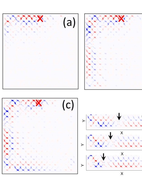
Figure 11: (Color online) snap shots of a transverse magnetic moment after the a.c. field is applied at $t=0$; (a): $t=100$ns, (b): 200ns, (c) 300ns, (d) t=350, 352, 354ns. The frequency of the a.c. field and the static out-of-plane field is set to 654GHz and 800 Oe respectively. Color specify the sign of the transverse moment (red is for positive and blue is for negative). In (a-c), the spin density propagates in the counterclockwise direction, while, in (d), the node of the transverse moment (indicated by black arrows) moves in the clockwise direction; the phase velocity is opposite to the group velocity.

Fig. 9(a) shows a contour plot of the integrated power spectrum $A(\omega)$ as a function of the static out-of-plane field ($\geq$ 620 Oe). The initial pulse field is applied at the center of the superlattice. On the whole, the spectrum composes of three major responance frequency regimes; for H=$800$Oe, these three are ranged over 6$\sim$7GHz, 8.5$\sim$9GHz, and 9.5$\sim$11GHz respectively. Fig. 9(b) shows a contour plot of the density of states of volume-mode bands obtained from a spin-wave calculation on the same magnetic superlattice. Since the superlattice has 12 spins within each unit cell, it has 12 volume-mode bands. A comparison reveals that the first and second lowest resonance frequency regimes found in $A(\omega)$ includes two volume-mode bands respectively, while the third resonance frequency regime includes remaining 8 bands. A comparison with the spin-wave analyses also shows that the lowest two volume-mode bands can be well reproduced by the two-orbital tight-binding model introduced in eqs. (12,13); the lowest two bands are mainly composed of the in-phase orbital wavefunction localized at the nearest neighbor $x$-link and that of the $y$-link. Thereby, they are essentially same as the lowest two bands found in the sec. II ($H>H_{c}$), and thus we expect that the chiral edge mode goes across a band gap between these two (see Fig. 5).

Fig. 10(a) shows the integrated power spectra within the lowest resonance frequency regime. The spectrum for volume-mode bands (spectrum obtained with the initial pulse field applied at the center of the system) comprises of two major humps; one ranges from 6.0GHz to 6.4GHz and the other from 6.6GHz to 6.8GHz (black line in Fig. 10(a)). They correspond to the lowest two volume-mode bands. In fact, the spatial-resolved power spectra within these two frequency regimes are extended over the system (Fig. 10(b,c)), while the system remains intact against those pulse fields within a band gap regime 6.4GHz $\sim$ 6.6GHz. (Fig. 10(d)). When the pulse field is applied at the boundary of the system, however, the integrated spectrum has a significant weight within the band gap regime (red line in Fig. 10(a)). The spatial-resolved spectrum reveals that these weight mainly come from the boundary of the system (Fig. 10(e)), indicating the existence of edge modes within the band gap regime.

A key feature of the chiral edge mode is a unidirectional propagation of spin wave densities. To confirm this feature, we perform another micromagnetic simulation, applying a.c. transverse field locally at the boundary of the system (red crossed point in Fig. 8). We set an external frequency of the a.c. field within the band gap regime; $\omega=6.54$GHz. Fig. 11 shows several snap shots of the transverse magnetization ($m_{x}(X,Y,t)$) taken after the a.c. field is applied from $t=0$. The snap shots clearly demonstrate a unidirectional propagation of spin densities in the counterclockwise direction. The direction of the propagation is consistent with the sign of the group velocity of the chiral edge modes proposed in the preceding sections. From the snap shots, the group velocity can be estimated to be one unit cell ($a$; linear dimension of the unit cell) per 10 ns, which is on the same order of the band gap divided by $2\pi/a$ (the gap $\sim$ 0.2GHz). The phase velocity of the edge mode is 10 times faster than the group velocity and its sign sometimes becomes opposite to that of the group velocity (Fig. 11(d)). This observation is also consistent with the chiral spin edge mode proposed in the ring model; the chiral dispersion goes across the first Brillouin zone once (Fig. 5(a,b)), so that the sign of the phase velocity can be either same or opposite to the group velocity.

V Summary and Discussion

V.1 summary of our findings

In this paper, we theoretically explored a realization of topological chiral edge mode for magnetostatic spin wave in patterned magnetic thin films, where magnetic clusters (either rings or disks) form a two-dimensional square lattice. Without external magnetic field, the ground-state spin configuration takes a form of circular vortices within each ring or disk, respecting the square-lattice translational symmetry. Due to the magnetic shape anisotropy, spin-wave excitations are fully gapped at the zero field. When an out-of-plane magnetic field is increased up to a saturation field, forward spin-wave modes within each ring or disk become significantly softened. With the four-fold rotational symmetry of the square lattice, these modes can be regarded as either $s$-wave, $p_{x}\pm ip_{y}$-wave or $d_{x^{2}-y^{2}}$-wave-like ‘atomic orbitals’. When inter-cluster transfer integrals among these orbital wave functions are larger than frequency spacings among their atomic orbital levels, the band-inversion between the parity-even atomic orbital level ($s$-wave or $d$-wave) and parity-odd orbital level ($p_{\pm}$-wave) leads to a chiral volume-mode bands with finite Chern integers. This results in a chiral (counterclockwise) edge mode within a band gap for the volume-mode bands.

When the system is fully polarized by the out-of-plane field, a strong four-fold rotational anisotropy of the demagnetization coefficient leads to another effective two-bands model. The model is composed of soft magnons localized on the nearest neighbor $x$-link and that on the $y$-link. Since atomic orbital levels for these two are same due to the square-lattice symmetry, transfer integrals between neighboring soft magnons immediately lead to a band inversion mechanism. The two-orbital model has massive Dirac cone like spectra at two inequivalent $X$-points, inside which a chiral (counterclockwise) edge mode appears. The massive Dirac spectra and the edge mode persist for a wide range above the saturation field. This feature is also justified by micromagnetic simulations.

V.2 applications to other systems

In reality, the square-lattice models studied in this paper could be placed on some magnetic substrates. Also, it is experimentally much easier to engrave only a surface of a plane thin film with some periodic structuring. Adeyeye ; Gulyaev The arguments employed in this paper can be also applicable to such systems. For example, consider that a surface of a magnetic film has a number of gutters/cambers forming a square lattice, Fig. 12(a)/(b) respectively. Due to the magnetostatic energy, moments in thinner film regions have stronger easy-plane anisotropy than those in thicker film regions. Therefore, on applying and increasing an out-of-plane field, the moments in thinner regions are expected to become fully polarized along the field at the highest saturation field, while those in the thicker regions do so at the lowest saturation field. This means that, in a system shown in Fig. 12(a), magnons at the gutter region becomes softened around the highest saturation field, forming atomic orbital wave functions. In the other system shown in Fig. 12(b), soft modes near the lowest saturation field are from the camber region. In the presence of the four-fold-rotational symmetry, these orbital wave functions play the role of either parity-even ($d_{x^{2}-y^{2}}$ or $s$-waves) orbitals and parity-odd ($p_{\pm}$-waves) orbitals, or the in-phase orbitals localized on the nearest neighbor $\mu$-link ($\mu=x,y$). Thus, provided that neighboring gutters/cambers are proximate to each other, the band inversion mechanisms described in this paper are expected to be valid, leading to a band gap of soft volume-mode bands with a chiral (counterclockwise) edge mode.

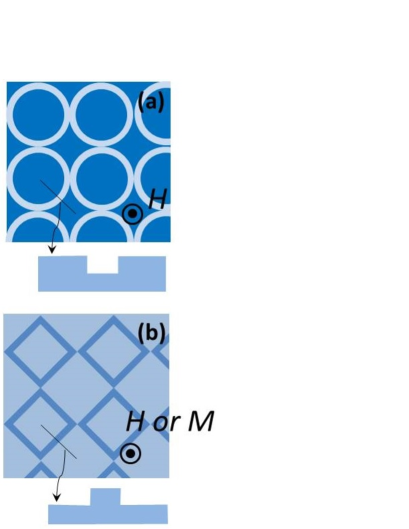
Figure 12: (Color online) Patterned magnetic films with periodically aligned gutters (a) or cambers (b). Without magnetic crystalline anisotropy (MCA), spins at the thinner regions feel stronger easy-plane anisotropy than those at that thicker regions.

The argument is also applicable to thin film ferromagnetic materials with perpendicular magnetic anisotropy (PMA), where relative strength between magnetic shape anisotropy and magnetic crystalline anisotropy (MCA) is controlled by the film thickness. Hubert In an ultrathin film limit (several atomic monolayer), the MCA with easy-axis (out-of-plane) anisotropy dominates over the magnetostatic energy with easy-plane anisotropy, so that magnetic moments are polarized vertically to the plane. It has been experimentally known that increasing film thickness leads to spin-reorientation transition from out-of-plane magnetization to in-plane magnetization, which indicates that magnetic shape anisotropy overcomes the MCA in thicker region. Qiu Around the critical thickness, gapped spin wave modes are expected to become significantly softened.

Regarding the film thickness as alternative to the magnetic field, one could also realize topological chiral spin-wave edge modes without any external magnetic field. For example, consider that a surface of a thin-film PMA material is engraved with cambers with a lattice periodicity as in Fig. 12(b). Suppose that a film-thickness of the camber region is chosen near the critical thickness of the material, so that magnons around camber regions are sufficiently softened, forming orbital wave functions such as $s$, $p_{\pm}$, $d$-waves or in-phase orbitals. When neighboring cambers are put in close contact with one another as in Fig. 12(b), exchange processes due to magnetic dipole interaction give rise to considerable transfer integrals among these orbital wave functions. Although their atomic orbital levels within each camber could be also modified by the MCA energy, we can still expect that larger transfer integrals induce the similar type of the band inversion as discussed in this paper.

V.3 a possible experimental method for detecting the chiral spin-wave edge mode

The proposed chiral edge modes can be experimentally detected in terms of two coils put along the boundary of the 2-$d$ magnetic superlattice; one is for an input and the other for an output (see Fig. 3(c)). They are spatially separated by tens of the unit cell (for example, 30 unit cells; 0.3mm for a unit cell of 10$\mu$m size). An a.c. electric current in the input coil induces an a.c. magnetic field near the coil, exciting spin waves (electric input). When a frequency of the a.c. current is chosen within the band gap regime, the chiral edge mode will be selectively excited. The excited spin wave propagates along the chiral edge mode and reaches the output coil after a certain time delay (e.g. 0.3$\mu$s according to the simulation in sec. IV). When the spin wave reaches around the output coil, an a.c. electric current with the same frequency will be induced in the output coil (electric detection). When the two coils are exchanged, the spin wave never reaches the output coil, unless it could propagate all the way around the boundary without being dissipated.

When the thickness of the 2-$d$ magnetic superlattice is much larger than short-range exchange interaction length, the input a.c. current can excite not only the proposed topological chiral edge modes but also the conventional chiral surface mode; Damon-Eshbach (DE) surface mode. In such a case, the output a.c. current comprises of two contributions; one from the topological chiral edge mode and the other from the DE mode. In general, these two modes have a number of quantitatively different features. First of all, these modes have quite different group velocities; the group velocity of the topological edge mode linearly depends on the superlattice unit cell size, while that of the DE mode doesn’t depend on the unit cell size. The topological edge mode has a resonance frequency within a band gap regimes for volume mode bands, which is determined by the magnetic superlattice. On the one hand, a resonance frequency regime of the DE mode is determined only by the out-of-plane magnetization $M$ and field $H$, $H<\omega<\sqrt{H(H+4\pi M)}$. When the external frequency is changed within the band gap regime, the phase velocity of the topological mode often changes its sign (see Fig. 5(a,b)), while that of DE mode doesn’t. In actual experiments, we can exploit these distinct features, so as to distinguish the contribution of the topological edge mode from that of the conventional DE surface mode. For example, we can easily differentiate these two contributions in time, by changing the distance between the input and output coils. We can further reduce one or the other, by changing an external frequency of the input a.c. current. Also, by changing the external frequency within the band gap regime, we can see the phase velocity of the topological mode change its sign.

Appendix A Holstein-Primakoff approximation and topological Chern integer for magnetostatic spin waves

In this paper, we considered that magnetic clusters, either thin rings or circular disks, form a 2-$d$ periodic lattice; magnetic superlattice. To study their magnetostatics and dynamics, we used discrete spin models; each cluster is discretized into many spins with small volume element, where the spins are coupled with one another only via magnetic dipole-dipole interaction. We first minimize the magnetostatic energy of the discrete spin models,

$$E \equiv-\frac{1}{2}\big{(}\Delta V\big{)}^{2}\sum^{i\neq j}_{i,j}\sum_{a,b=x,y,z}M_{a}({\bm{r}}_{i})f_{ab}({\bm{r}}_{i}-{\bm{r}}_{j})M_{b}({\bm{r}}_{j})$$

$$\hskip 14.22636pt-H\Delta V\sum_{i}M_{z}({\bm{r}}_{i}),$$ (16)

to determine a classical spin configuration ${\bm{M}}_{0}({\bm{r}})$. ${\bm{r}}_{i}$ specifies a spatial location of a ferromagnetic spin with fixed size of moment $|{\bm{M}}({\bm{r}}_{i})|=M_{s}$. $f_{ab}({\bm{r}}_{i}-{\bm{r}}_{j})$ is the magnetic dipole-dipole interaction between spin at ${\bm{r}}_{i}$ and spin at ${\bm{r}}_{j}$;

$$f_{ab}({\bm{r}})\equiv-\frac{1}{4\pi}\Big{(}\frac{\delta_{a,b}}{|{\bm{r}}|^{3}}-\frac{3r_{a}r_{b}}{|{\bm{r}}|^{5}}\Big{)}.$$

$\Delta V$ denotes a volume element for each spin, whose linear dimension is of the same order of short-ranged exchange length $l_{\rm ex}$; For YIG and Iron, $l_{\rm ex}=18.4$ nm and $2.9$ nm respectively.

Without the field, the energetically stable spin configuration is an array of circular magnetic vortices, Hubert ; Cowburn ; Shinjo respecting the periodicity of the square lattice. Under the out-of-plane field, the configurations acquire finite out-of-plane moments, which will be fully polarized above a saturation field. To obtain spin-wave modes, we linearize the corresponding Landau-Lifshitz equation in favor of fluctuation fields around the classical spin configuration.

In the discrete spin models, the Landau-Lifshitz equation take a form of,

$$\partial_{t}M_{a}({\bm{r}}_{i}) =\epsilon_{abc}\Big{[}-H\delta_{b,z}$$

$$\hskip 28.45274pt-\Delta V\sum_{j\neq i}f_{bd}({\bm{r}}_{i}-{\bm{r}}_{j})M_{d}({\bm{r}}_{j})\Big{]}M_{c}({\bm{r}}_{i}).$$

Note that the right hand side suggests that the saturation field and characteristic spin-wave resonance frequency are scaled as $M_{s}\Delta V/l^{3}$. Here $l$ denotes a distance between the nearest neighbor spins in the discrete spin models and $1/l^{3}$ comes from the dipole-dipole interaction between them. The small volume element for each spin should be spatially isotropic, such that the discrete spin models can approximately describe the Maxwell equation for magnetic continuum media. This requires $\Delta V\simeq l^{3}$. As a result, characteristic spin-wave resonance frequencies and saturation field are scaled only by the saturation magnetization of a constituent material.

The equation of motion is linearized with respect to a small transverse field ${\bm{m}}_{\perp}({\bm{r}})$ with ${\bm{m}}_{\perp}({\bm{r}})\equiv{\bm{M}}({\bm{r}})-{\bm{M}}_{0}({\bm{r}})$ and ${\bm{m}}_{\perp}({\bm{r}})\perp{\bm{M}}_{0}({\bm{r}})$. With a local spin frame in which the classical configuration ${\bm{M}}_{0}({\bm{r}})$ becomes fully polarized along the $z$-direction, i.e. ${\bm{R}}({\bm{r}}){\bm{M}}_{0}({\bm{r}})=M_{s}{\bm{e}}_{z}$ and ${\bm{R}}({\bm{r}}){\bm{m}}_{\perp}({\bm{r}})={\bm{m}}({\bm{r}})$, the two transverse moments in the rotated frame ${\bm{m}}({\bm{r}})=(m_{x}({\bm{r}}),m_{y}({\bm{r}}))$ comprise creation/annihilation operator for spin wave (magnon);

$$m_{\mp}({\bm{r}})\equiv m_{x}({\bm{r}})\pm im_{y}({\bm{r}}).$$

With this magnon field, the linearized equation reduces to a generalized Hermitian eigenvalue problem,

$$i\partial_{t}\left(\begin{array}[]{c}m_{-}({\bm{r}}_{i})\\ m_{+}({\bm{r}}_{i})\\ \end{array}\right)=\sum_{j}{\bm{\sigma}}_{3}\!\ \big{(}{\bm{H}}\big{)}_{{\bm{r}}_{i},{\bm{r}}_{j}}\left(\begin{array}[]{c}m_{-}({\bm{r}}_{j})\\ m_{+}({\bm{r}}_{j})\\ \end{array}\right),$$ (21)

${\bm{\sigma}}_{3}$ is a diagonal matrix which takes $+1$ in the particle space ($m_{+}$) and $-1$ in the hole space ($m_{-}$), reflecting the fact that the magnon obeys the bose statistics. In this particle-hole space, the Hermite matrix is given by the following $2$ by $2$ matrix,

$$\big{(}{\bm{H}}\big{)}_{{\bm{r}}_{i},{\bm{r}}_{j}} \equiv-M_{s}\alpha({\bm{r}}_{i})\delta_{{\bm{r}}_{i},{\bm{r}}_{j}}\left(\begin{array}[]{cc}1&\\ &1\\ \end{array}\right)$$ (24)

$$-M_{s}\Delta V(1-\delta_{{\bm{r}}_{i},{\bm{r}}_{j}})\left(\begin{array}[]{cc}f_{++}({\bm{r}}_{i},{\bm{r}}_{j})&f_{+-}({\bm{r}}_{i},{\bm{r}}_{j})\\ f_{-+}({\bm{r}}_{i},{\bm{r}}_{j})&f_{--}({\bm{r}}_{i},{\bm{r}}_{j})\\ \end{array}\right).$$ (27)

$\alpha({\bm{r}}_{i})$ denotes the demagnetization coefficient including the static out-of-plane field component;

$$\alpha({\bm{r}}_{i}){\bm{M}}_{0}({\bm{r}}_{i})=-\Delta V\sum_{j\neq i}{\bm{f}}({\bm{r}}_{i}-{\bm{r}}_{j}){\bm{M}}_{0}({\bm{r}}_{j})-H{\bm{e}}_{z},$$

where the equality holds true provided that the classical spin configuration gives a local minimum of the magnetostatic energy, eq. (16). $f_{\mu\nu}({\bm{r}}_{i},{\bm{r}}_{j})$ ($\mu=\pm$) in eq. (27) represents ‘exchange’ process between ${\bm{r}}_{i}$ and ${\bm{r}}_{j}$, which gives rise to propagation of magnon excitation under a background of the classical spin configuration. The $2$ by $2$ matrix is defined as

$$\left(\begin{array}[]{cc}f_{++}({\bm{r}},{\bm{r}}^{\prime})&f_{+-}({\bm{r}},{\bm{r}}^{\prime})\\ f_{-+}({\bm{r}},{\bm{r}}^{\prime})&f_{--}({\bm{r}},{\bm{r}}^{\prime})\\ \end{array}\right)$$ (30)

$$\ =\frac{1}{2}\left(\begin{array}[]{cc}1&i\\ 1&-i\\ \end{array}\right)\left(\begin{array}[]{cc}f_{xx}({\bm{r}},{\bm{r}}^{\prime})&f_{xy}({\bm{r}},{\bm{r}}^{\prime})\\ f_{yx}({\bm{r}},{\bm{r}}^{\prime})&f_{yy}({\bm{r}},{\bm{r}}^{\prime})\\ \end{array}\right)\left(\begin{array}[]{cc}1&1\\ -i&i\\ \end{array}\right).$$ (37)

$f_{\alpha\beta}({\bm{r}},{\bm{r}}^{\prime})$ ($\alpha,\beta=x,y,z$) in the right hand side denotes the dipolar interaction in the rotated frame,

$${\bm{f}}({\bm{r}},{\bm{r}}^{\prime})\equiv{\bm{R}}({\bm{r}}){\bm{f}}({\bm{r}}-{\bm{r}}^{\prime}){\bm{R}}^{t}({\bm{r}}^{\prime}).$$ (38)

To begin with, consider spin-wave exctitations in a circular ring. We treat the ring as a one-dimensional chain of many spins which are equally spaced from respective neighborings and spins along the ring is parameterized by an angle i.e. ${\bm{r}}_{j}=r(\cos\theta_{j},\sin\theta_{j},0)$ with $\theta_{j}=\frac{2\pi j}{M}$ $(j=1,2,\cdots,M)$. ‘$r$’ denotes the radius of the ring. The classical spin configuration minimizing the magnetostatic energy eq. (16) respects the circular symmetry,

$${\bm{M}}_{0}({\bm{r}}_{j})=M_{s}(-\sin\varphi\sin\theta_{j},\sin\varphi\cos\theta_{j},\cos\varphi).$$

$\varphi$ denotes a relative angle between each spin and the external magnetic field, which is independent from $j$ due to the circular symmetry. To introduce a magnon and its Hamiltonian in a ring, we take a following local spin frame in eqs. (27-38),

$${\bm{R}}({\bm{r}}_{j})=\left(\begin{array}[]{ccc}1&&\\ &\cos\varphi&-\sin\varphi\\ &\sin\varphi&\cos\varphi\\ \end{array}\right)\left(\begin{array}[]{ccc}\cos\theta_{j}&\sin\theta_{j}&\\ -\sin\theta_{j}&\cos\theta_{j}&\\ &&1\\ \end{array}\right).$$ (45)

Under this gauge, the right hand side of eq. (38) depends only on a relative angle between two magnetic elements along the ring;

$${\bm{f}}({\bm{r}}_{i},{\bm{r}}_{j}) ={\bm{f}}(\theta_{i}-\theta_{j})=-\frac{1}{32\pi a^{3}|\sin\frac{\theta_{i}-\theta_{j}}{2}|^{3}}\Bigg{\{}\left(\begin{array}[]{ccc}c_{\theta_{i}-\theta_{j}}&s_{\theta_{i}-\theta_{j}}c_{\varphi}&s_{\theta_{i}-\theta_{j}}s_{\varphi}\\ -s_{\theta_{i}-\theta_{j}}c_{\varphi}&c_{\theta_{i}-\theta_{j}}c^{2}_{\varphi}+s^{2}_{\varphi}&(c_{\theta_{i}-\theta_{j}}-1)c_{\varphi}s_{\varphi}\\ -s_{\theta_{i}-\theta_{j}}s_{\varphi}&(c_{\theta_{i}-\theta_{j}}-1)c_{\varphi}s_{\varphi}&s^{2}_{\varphi}c_{\theta_{i}-\theta_{j}}+c^{2}_{\varphi}\\ \end{array}\right)$$ (49)

$$\hskip 85.35826pt-\frac{3}{2}\left(\begin{array}[]{ccc}-(1-c_{\theta_{i}-\theta_{j}})&s_{\theta_{i}-\theta_{j}}c_{\varphi}&s_{\theta_{i}-\theta_{j}}s_{\varphi}\\ -s_{\theta_{i}-\theta_{j}}c_{\varphi}&(c_{\theta_{i}-\theta_{j}}-1)c^{2}_{\varphi}&(c_{\theta_{i}-\theta_{j}}-1)c_{\varphi}s_{\varphi}\\ -s_{\theta_{i}-\theta_{j}}s_{\varphi}&c_{\varphi}s_{\varphi}(c_{\theta_{i}-\theta_{j}}-1)&s^{2}_{\varphi}(c_{\theta_{i}-\theta_{j}}-1)\\ \end{array}\right)\Bigg{\}}$$ (53)

with $c_{\theta_{i}-\theta_{j}}\equiv\cos(\theta_{i}-\theta_{j})$, $s_{\theta_{i}-\theta_{j}}\equiv\sin(\theta_{i}-\theta_{j})$, $c_{\varphi}\equiv\cos\varphi$, and $s_{\varphi}\equiv\sin\varphi$. The demagnetization coefficient in an isolated ring also respects the circular symmetry; $\alpha({\bm{r}}_{j})=\alpha$. Thus, the magnon Hamiltonian for a circular ring depends only on the relative angle;

$$i\partial_{t}\left(\begin{array}[]{c}m_{-}(\theta_{i})\\ m_{+}(\theta_{i})\\ \end{array}\right)=\sum^{M}_{j=1}{\bm{\sigma}}_{3}\!\ \big{(}{\bm{H}}\big{)}_{\theta_{i}-\theta_{j}}\left(\begin{array}[]{c}m_{-}(\theta_{j})\\ m_{+}(\theta_{j})\\ \end{array}\right),$$ (58)

Correspondingly, the spin-wave excitations in a ring are characterized by the angular momentum variable $q_{J}=\frac{2\pi n_{J}}{M}$ $(n_{J}=-\frac{M}{2},-\frac{M}{2}+1,\cdots,\frac{M}{2})$ associated with the circular symmetry;

$$\left(\begin{array}[]{c}m_{-}(\theta_{i})\\ m_{+}(\theta_{i})\\ \end{array}\right)=\sum_{n_{J}}e^{in_{J}\theta_{i}}\left(\begin{array}[]{c}m_{-}(n_{J})\\ m_{+}(-n_{J})\\ \end{array}\right).$$ (63)

The linearized equation is given by

$$i\partial_{t}\left(\begin{array}[]{c}m_{-}(n_{J})\\ m_{+}(-n_{J})\\ \end{array}\right)={\bm{\sigma}}_{3}\!\ \big{(}{\bm{H}}\big{)}_{n_{J}}\left(\begin{array}[]{c}m_{-}(n_{J})\\ m_{+}(-n_{J})\\ \end{array}\right),$$ (68)

with

$$({\bm{H}})_{n_{J}}\equiv\sum_{j}e^{in_{J}\theta_{j}}({\bm{H}})_{\theta_{j}}.$$

The 2 by 2 Hermite matrix $({\bm{H}})_{n_{J}}$ is diagonalized for each angular momentum in terms of canonical transformation (2 by 2 paraunitary matrix);

$$({\bm{H}})_{n_{J}}{\bm{t}}_{n_{J}}={\bm{\sigma}}_{3}\!\ {\bm{t}}_{n_{J}}E_{n_{J}}.$$ (69)

with a proper normalization ${\bm{t}}^{\dagger}_{n_{J}}{\bm{\sigma}}_{3}{\bm{t}}_{n_{J}}=1$. Positive definite $E_{n_{J}}$ stands for a resonance frequency for the spin-wave excitations in a circular ring. Respective spin-wave mode is represented by the two-component vector in the particle-hole space ${\bm{t}}_{n_{J}}$; the linearized equation of motion eq. (58) is satisfied by

$$\psi_{q_{J}}(\theta_{j})={\bm{t}}_{n_{J}}\!\ e^{in_{J}\theta_{j}-iE_{n_{J}}t}$$ (70)

with $q_{J}\equiv\frac{2\pi n_{J}}{M}$. Eq. (70) with $n_{J}=-\frac{M}{2},\cdots,\frac{M}{2}-1,\frac{M}{2}$ comprise ‘atomic orbital’ wavefunctions within a circular ring, which are classified by the total angular momentum $q_{J}$;

$$\psi_{q_{J}}(\theta_{j}+\theta_{m})=e^{iq_{J}m}\psi_{q_{J}}(\theta_{j}).$$

These wavefunctions gives us bases for tight-binding descriptions of spin-wave excitations in the magnetic superlattice.

To obtain spin-wave dispersion relations for volume modes and edge modes in the magnetic superlattices, we diagonalize eq. (27) with a periodic boundary condition along the $x$-direction and an open boundary condition along the $y$-direction. A system typically contains $9$-$18$ square-lattice unit cell along the $y$-direction. We minimize the magnetostatic energy, respecting the periodicity of the square lattice, ${\bm{M}}_{0}({\bm{r}}+{\bm{e}}_{x})={\bm{M}}_{0}({\bm{r}})$. So do $\alpha({\bm{r}})$, ${\bm{R}}({\bm{r}})$ and $({\bm{H}})_{{\bm{r}}_{i},{\bm{r}}_{j}}$; $({\bm{H}})_{{\bm{r}}_{i}+{\bm{e}}_{x},{\bm{r}}_{j}}=({\bm{H}})_{{\bm{r}}_{i},{\bm{r}}_{j}-{\bm{e}}_{x}}$. Correspondingly, we diagonalize the following fourier-transformed Hamiltonian,

$$({\bm{H}}_{k})_{{\bm{r}}_{i},{\bm{r}}_{j}} =-M_{s}\alpha({\bm{r}}_{i})\delta_{{\bm{r}}_{i},{\bm{r}}_{j}}$$

$$\ \ \ -M_{s}\Delta V\left(\begin{array}[]{cc}f_{k,++}({\bm{r}}_{i},{\bm{r}}_{j})&f_{k,+-}({\bm{r}}_{i},{\bm{r}}_{j})\\ f_{k,-+}({\bm{r}}_{i},{\bm{r}}_{j})&f_{k,--}({\bm{r}}_{i},{\bm{r}}_{j})\\ \end{array}\right),$$ (73)

with

$$f_{k,\sigma\sigma^{\prime}}({\bm{r}},{\bm{r}}^{\prime}) =e^{-ik({\bm{r}}-{\bm{r}}^{\prime})_{x}}\times$$

$$\ \ \ \sum_{\bm{b}}(1-\delta_{{\bm{r}},{\bm{r}}^{\prime}-{\bm{b}}})f_{\sigma\sigma^{\prime}}({\bm{r}},{\bm{r}}^{\prime}-{\bm{b}})e^{-ik{\bm{b}}_{x}}.$$

with $\sigma,\sigma^{\prime}=\pm$. The summation over the lattice translational vector ${\bm{b}}$ is taken only along the $x$-direction and is over a finite range ${\bm{b}}\equiv n{\bm{e}}_{x}$ with $-10\leq n\leq 10$. Provided that the classical spin configuration ${\bm{M}}_{0}({\bm{r}}_{i})$ gives a local minimum for the magnetostatic energy, the linearized Hamiltonian is paraunitarily equivalent to a positive definite diagonal matrix ${\bm{E}}_{k}$: ${\bm{T}}^{\dagger}_{k}{\bm{H}}_{k}{\bm{T}}_{k}={\bm{E}}_{k}$ with ${\bm{T}}^{\dagger}_{k}{\bm{\sigma}}_{3}{\bm{T}}_{k}={\bm{\sigma}}_{3}$. Each diagonal element in ${\bm{E}}_{k}$ and corresponding column vector in ${\bm{T}}_{k}$ gives a resonance frequency and wave function for a volume mode and edge mode as a function of the wave vector $k$ along the $x$-direction. With the normalization condition of ${\bm{T}}_{k}$ in mind, an amplitude of the wave function for the $n$-th eigen mode at ${\bm{r}}_{i}$ is defined as $\sum_{\sigma=\pm}\sigma|({\bm{T}}_{k})_{({\bm{r}}_{j},\sigma|n)}|^{2}$. We regard the mode as an edge mode, when more than $70\%$ of the amplitude is localized along the boundaries of the system (see also the captions of Figs. 3, 7). Otherwise, we observed that wave functions are usually extended over the system, and thus can be regarded as volume modes.

Dispersion relations for the volume modes are also obtained from calculations with periodic boundary conditions imposed on both $x$ and $y$-direction. The classical ground-state spin configuration respects the periodicity of the square lattice, ${\bm{M}}_{0}({\bm{r}}+{\bm{e}}_{x})={\bm{M}}_{0}({\bm{r}}+{\bm{e}}_{y})={\bm{M}}_{0}({\bm{r}})$. We diagonalize eq. (73) with $k$ being replaced by ${\bm{k}}=(k_{x},k_{y})$, in terms of a paraunitary transformation ${\bm{T}}_{\bm{k}}$;

$$f_{{\bm{k}},\sigma\sigma^{\prime}}({\bm{r}},{\bm{r}}^{\prime}) =e^{-i{\bm{k}}({\bm{r}}-{\bm{r}}^{\prime})}\times$$

$$\ \ \ \sum_{\bm{b}}(1-\delta_{{\bm{r}},{\bm{r}}^{\prime}-{\bm{b}}})f_{\sigma\sigma^{\prime}}({\bm{r}},{\bm{r}}^{\prime}-{\bm{b}})e^{-i{\bm{k}}{\bm{b}}},$$

with ${\bm{b}}=n{\bm{e}}_{x}+m{\bm{e}}_{y}$ and $-10\leq n,m\leq 10$. The topological Chern integer for the $j$-th volume mode band is defined by the $j$-the column vector of the paraunitary matrix ${\bm{T}}_{\bm{k}}$ as

$$c_{j}\equiv\frac{i\epsilon_{\mu\nu}}{2\pi}\int_{\rm BZ}d^{2}{\bm{k}}\!\ {\rm Tr}\Big{[}{\bm{\Gamma}}_{j}{\bm{\sigma}}_{3}\big{(}\partial_{k_{\mu}}{\bm{T}}^{\dagger}_{\bm{k}}\big{)}{\bm{\sigma}}_{3}\big{(}\partial_{k_{\nu}}{\bm{T}}_{\bm{k}}\big{)}\Big{]}.$$

Here ${\bm{\Gamma}}_{j}$ takes $+1$ in the $(j,j)$ component while $0$ otherwise. $c_{j}$ takes an integer and describes a topological structure of a wave function for the $j$-th volume mode band in the two-dimensional Brillouin zone (BZ). SO1 ; TKKN ; Avron

Appendix B two-orbital model valid above the saturation field

When the classical spin configuration is fully polarized along the out-of-plane field, demagnetization field at the four corner of a ring, ${\bm{r}}_{j}={\bm{b}}_{j}+r(\cos\theta_{j},\sin\theta_{j})$ with $\theta_{j}=0,\frac{\pi}{2},\pi,\frac{3\pi}{2}$, is much stronger than those in the others. Here ${\bm{b}}_{j}$ denote a coordinate of a center of the ring at which a spin at ${\bm{r}}_{j}$ is included. $r$ is a radius of the ring (Fig. 13). As a result, soft volume mode bands are mainly composed of spins localized at $\theta_{j}=0,\frac{\pi}{2},\pi,\frac{3\pi}{2}$. In such a case, exchange process between nearest neighbor rings becomes even larger than that within a same ring. We thus take into account the former exchange process first, to introduce atomic orbital wave functions defined on a link connecting two nearest neighboring rings.

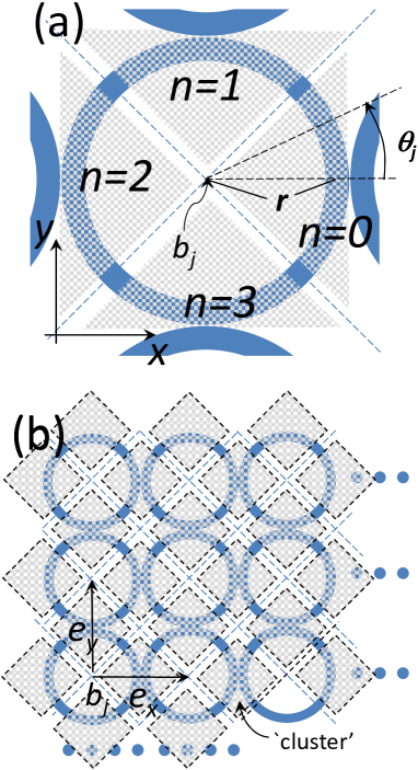
Figure 13: (Color online) (a) Ring is decomposed into four quadrants (grey shadow regions), which are ranged as $-\frac{\pi}{4}\leq\theta_{j}\leq\frac{\pi}{4}$ ($n=0$), $\frac{\pi}{4}\leq\theta_{j}\leq\frac{3\pi}{4}$ ($n=1$), $\frac{3\pi}{4}\leq\theta_{j}\leq\frac{5\pi}{4}$ ($n=2$), $\frac{5\pi}{4}\leq\theta_{j}\leq\frac{7\pi}{4}$ ($n=3$) respectively with ${\bm{r}}_{j}={\bm{b}}_{j}+r(\cos\theta_{j},\sin\theta_{j})$. Here ${\bm{b}}_{j}$ denotes a center of the ring and $r$ is a radius of the ring. (b) One quadrant in a ring and its closest quadrant in the nearest neighbor ring are combined together, to form a cluster (grey shadow region encompassed by a black dotted line). The cluster thus defined is centered at ${\bm{b}}_{j}+\frac{{\bm{e}}_{x}}{2}$ (a mid-point of the nearest neighbor $x$-link) or ${\bm{b}}_{j}+\frac{{\bm{e}}_{y}}{2}$ (a mid-point of the $y$-link), where ${\bm{e}}_{x}$ and ${\bm{e}}_{y}$ are the basic translational vectors.

Specifically, we first decompose every ring, ${\bm{r}}_{j}={\bm{b}}_{j}+r(\cos\theta_{j},\sin\theta_{j})$, into four quadrants, which are ranged as $-\frac{\pi}{4}\leq\theta_{j}\leq\frac{\pi}{4}$, $\frac{\pi}{4}\leq\theta_{j}\leq\frac{3\pi}{4}$, $\frac{3\pi}{4}\leq\theta_{j}\leq\frac{5\pi}{4}$, $\frac{5\pi}{4}\leq\theta_{j}\leq\frac{7\pi}{4}$ respectively (Fig. 13(a)). We then combine one quadrant in a ring ($-\frac{\pi}{4}\leq\theta_{j}\leq\frac{\pi}{4}$ with ${\bm{b}}_{j}$ or $\frac{\pi}{4}\leq\theta_{j}\leq\frac{3\pi}{4}$ with ${\bm{b}}_{j}$) and its closest quadrant of the nearest neighboring ring ($\frac{3\pi}{4}\leq\theta_{j}\leq\frac{5\pi}{4}$ with ${\bm{b}}_{j}+{\bm{e}}_{x}$ or $\frac{5\pi}{4}\leq\theta_{j}\leq\frac{7\pi}{4}$ with ${\bm{b}}_{j}+{\bm{e}}_{y}$ respectively), to make a ‘cluster’ (Fig. 13(b)). The cluster thus defined is centered at a middle point of the nearest neighbor $x$-link or that of the $y$-link (${\bm{b}}_{j}+\frac{{\bm{e}}_{x}}{2}$ or ${\bm{b}}_{j}+\frac{{\bm{e}}_{y}}{2}$ respectively). Correspondingly, we decompose the BdG Hamiltonian in eq. (27) into two parts, one is diagonal with respect to a cluster index and the other is off-diagonal with respect to the cluster index;

$$\big{(}{\bm{H}}\big{)}_{{\bm{r}}_{i},{\bm{r}}_{j}}=\big{(}{\bm{H}}_{0}\big{)}_{{\bm{r}}_{i},{\bm{r}}_{j}}+\big{(}{\bm{H}}_{1}\big{)}_{{\bm{r}}_{i},{\bm{r}}_{j}},$$ (74)

with

$$\big{(}{\bm{H}}_{0}\big{)}_{{\bm{r}}_{i},{\bm{r}}_{j}} =-M_{s}\alpha({\bm{r}}_{i})\delta_{{\bm{r}}_{i},{\bm{r}}_{j}}\left(\begin{array}[]{cc}1&\\ &1\\ \end{array}\right)-M_{s}\Delta V\times$$ (77)

$$\hskip 28.45274pt\delta_{[{\bm{r}}_{i}],[{\bm{r}}_{j}]}\!\ \eta_{{\bm{r}}_{i},{\bm{r}}_{j}}\left(\begin{array}[]{cc}f_{++}({\bm{r}}_{i},{\bm{r}}_{j})&f_{+-}({\bm{r}}_{i},{\bm{r}}_{j})\\ f_{-+}({\bm{r}}_{i},{\bm{r}}_{j})&f_{--}({\bm{r}}_{i},{\bm{r}}_{j})\\ \end{array}\right),$$ (80)

$$\big{(}{\bm{H}}_{1}\big{)}_{{\bm{r}}_{i},{\bm{r}}_{j}} =-M_{s}\Delta V\!\ \eta_{[{\bm{r}}_{i}],[{\bm{r}}_{j}]}\left(\begin{array}[]{cc}f_{++}({\bm{r}}_{i},{\bm{r}}_{j})&f_{+-}({\bm{r}}_{i},{\bm{r}}_{j})\\ f_{-+}({\bm{r}}_{i},{\bm{r}}_{j})&f_{--}({\bm{r}}_{i},{\bm{r}}_{j})\\ \end{array}\right),$$ (83)

where $\eta_{{\bm{r}}_{i},{\bm{r}}_{j}}\equiv 1-\delta_{{\bm{r}}_{i},{\bm{r}}_{j}}$, $\eta_{[{\bm{r}}_{i}],[{\bm{r}}_{j}]}\equiv 1-\delta_{[{\bm{r}}_{i}],[{\bm{r}}_{j}]}$ and $[{\bm{r}}_{i}]$ species a cluster in which a spin site ${\bm{r}}_{i}$ is included. Now that the spin configuration is fully polarized, we take the following frame in eq. (38),

$${\bm{R}}({\bm{r}}_{i})\equiv\left(\begin{array}[]{ccc}\cos\theta_{i}&\sin\theta_{i}&\\ -\sin\theta_{i}&\cos\theta_{i}&\\ &&1\\ \end{array}\right).$$ (88)

with ${\bm{r}}_{i}\equiv{\bm{b}}_{i}+r(\cos\theta_{i},\sin\theta_{i})$. With this rotated spin frame, the $2$ by $2$ transfer integrals is given as

$$\left(\begin{array}[]{cc}f_{++}({\bm{r}}_{i},{\bm{r}}_{j})&f_{+-}({\bm{r}}_{i},{\bm{r}}_{j})\\ f_{-+}({\bm{r}}_{i},{\bm{r}}_{j})&f_{--}({\bm{r}}_{i},{\bm{r}}_{j})\\ \end{array}\right)=\frac{1}{4\pi R^{3}}\!\ \Bigg{\{}-\left(\begin{array}[]{cc}e^{-i(\theta_{i}-\theta_{j})}&\\ &e^{i(\theta_{i}-\theta_{j})}\\ \end{array}\right)+\frac{3}{2}\left(\begin{array}[]{cc}e^{-i(\theta_{i}-\theta_{j})}&e^{-i(\theta_{i}+\theta_{j})+2i\varphi_{ij}}\\ e^{i(\theta_{i}+\theta_{j})-2i\varphi_{ij}}&e^{i(\theta_{i}-\theta_{j})}\\ \end{array}\right)\Bigg{\}}$$ (95)

with ${\bm{r}}_{j}\equiv{\bm{b}}_{j}+r(\cos\theta_{j},\sin\theta_{j})$, $R\equiv|{\bm{r}}_{i}-{\bm{r}}_{j}|$ and ${\bm{r}}_{i}-{\bm{r}}_{j}\equiv R(\cos\varphi_{ij},\sin\varphi_{ij})$. In the following, we first diagonalize ${\bm{H}}_{0}$ to introduce ‘orbital wave functions’ within each cluster. In terms of this orbital basis, we next include ${\bm{H}}_{1}$ as a inter-cluster transfer integrals.

To carry out this procedure systematically, we further decompose the diagonal part into two parts, ${\bm{H}}_{0}\equiv{\bm{H}}^{\prime}_{0}+{\bm{H}}^{\prime\prime}_{0}$, where $({\bm{H}}^{\prime}_{0})_{{\bm{r}}_{i},{\bm{r}}_{j}}$ is no-zero if and only if both ${\bm{r}}_{i}$ and ${\bm{r}}_{j}$ are within the same quadrant, while $({\bm{H}}^{\prime\prime}_{0})_{{\bm{r}}_{i},{\bm{r}}_{j}}$ is non-zero if ${\bm{r}}_{i}$ is in one quadrant and ${\bm{r}}_{j}$ is in the other; ${\bm{H}}^{\prime\prime}_{0}$ plays the part of exchange process between the nearest neighbor quadrants. Consider first the lowest eigen basis which diagonalizes ${\bm{H}}^{\prime}_{0}$;

$${\bm{H}}^{\prime}_{0}|u_{\pm,n,{\bm{b}}}\rangle={\bm{\sigma}}_{3}|u_{\pm,n,{\bm{b}}}\rangle(\pm E),$$ (96)

where $\langle u_{\nu,n,{\bm{b}}}|{\bm{\sigma}}_{3}|u_{\mu,n^{\prime},{\bm{b}}^{\prime}}\rangle=\nu\delta_{\nu,\mu}\delta_{n,n^{\prime}}\delta_{{\bm{b}},{\bm{b}}^{\prime}}$ with $\nu,\mu=\pm$. ${\bm{b}}$ and ${\bm{b}}^{\prime}$ denote spatial coordinate of (a center of) the ring to which the basis belongs, while the subscripts $n,n^{\prime}(=0,1,2,3)$ specify the quadrant to which the basis belongs. For example, $\langle{\bm{r}}_{j},\tau|u_{\pm,0,{\bm{b}}}\rangle$ is non-zero only when ${\bm{b}}={\bm{b}}_{j}$ and $-\frac{\pi}{4}\leq\theta_{j}\leq\frac{\pi}{4}$ with ${\bm{r}}_{j}={\bm{b}}_{j}+r(\cos\theta_{j},\sin\theta_{j})$, while $\langle{\bm{r}}_{j},\tau|u_{\pm,1,{\bm{b}}}\rangle$ is non-zero only when ${\bm{b}}={\bm{b}}_{j}$ and $\frac{\pi}{4}\leq\theta_{j}\leq\frac{3\pi}{4}$ and so on (see also fig. 13(a) for $n=2,3$). $|u_{+,n,{\bm{b}}}\rangle$ and $|u_{-,n,{\bm{b}}}\rangle$ are particle-hole pair to each other,

$$\langle{\bm{r}}_{i},\tau|u_{-,n,{\bm{b}}}\rangle=({\bm{\sigma}}_{1})_{\tau\tau^{\prime}}\langle u_{+,n,{\bm{b}}}|{\bm{r}}_{i},{\tau}^{\prime}\rangle,$$ (97)

with the particle-hole index $\tau=1,2$. Due to the four-fold rotational and square-lattice translational symmetries, the lowest eigen frequency in eq. (96), $E$, does not depend on $n$ and ${\bm{b}}$.

Now that $-\alpha({\bm{r}}_{j})$ in ${\bm{H}}^{\prime}_{0}$ has deep minima at $\theta_{j}=0,\frac{\pi}{2},\pi,\frac{3\pi}{2}$ with ${\bm{r}}_{j}={\bm{b}}_{j}+r(\cos\theta_{j},\sin\theta_{j})$, the lowest eigen basis is expected to be localized around these valley bottoms,

$$\big{\langle}{\bm{r}}_{j},\tau\big{|}u_{+,n,{\bm{b}}}\big{\rangle}\simeq\delta_{{\bm{b}},{\bm{b}}_{j}}\Big{(}\delta_{n,0}\delta_{\theta_{j},0}+\delta_{n,1}\delta_{\theta_{j},\frac{\pi}{2}}$$

$$\hskip 56.9055pt+\delta_{n,2}\delta_{\theta_{j},\pi}+\delta_{n,3}\delta_{\theta_{j},\frac{3\pi}{2}}\Big{)}\left(\begin{array}[]{cc}u\\ v\\ \end{array}\right)_{\tau}.$$ (100)

$(u,v)$ represents a two-component vector in the particle-hole space. Near (but above) the saturation field, the vector is equally-weighted in the particle-hole space,

$$\left(\begin{array}[]{c}u\\ v\\ \end{array}\right)\simeq\left(\begin{array}[]{c}i\\ -i\\ \end{array}\right)\ \ \ {\rm for}\ \ H\gtrsim H_{c}.$$ (105)

The relative phase between the particle-component ($u$; $\tau=1$) and the hole component ($v$; $\tau=2$) was taken $-1$, because a condensation of the soft magnon with eq. (105) results in an in-plane component which is tangential to the ring; the in-plane component of the classical spin configuration at $H<H_{c}$ takes the circular vortex structure within each ring. Note also that, in eq. (100), the relative phase among different quadrants was chosen to be $+1$, because of the rotated spin frame, eq. (88). In the high field limit, the vector is polarized in the particle space,

$$\left(\begin{array}[]{c}u\\ v\\ \end{array}\right)\rightarrow\left(\begin{array}[]{c}1\\ 0\\ \end{array}\right)\ \ \ {\rm for}\ \ H\rightarrow\infty.$$ (110)

In terms of the lowest eigen basis of ${\bm{H}}^{\prime}_{0}$, ${\bm{H}}_{0}$ takes a form;

$${\bm{H}}_{0}= \sum_{{\bm{b}}}\Big{\{}\left(\begin{array}[]{cccc}\gamma^{\dagger}_{0,{\bm{b}}}&\gamma^{\dagger}_{2,{\bm{b}}+{\bm{e}}_{x}}&\gamma_{0,{\bm{b}}}&\gamma_{2,{\bm{b}}+{\bm{e}}_{x}}\end{array}\right)\left(\begin{array}[]{cccc}E&t&0&s\\ t&E&s&0\\ 0&s&E&t\\ s&0&t&E\\ \end{array}\right)\left(\begin{array}[]{c}\gamma_{0,{\bm{b}}}\\ \gamma_{2,{\bm{b}}+{\bm{e}}_{x}}\\ \gamma^{\dagger}_{0,{\bm{b}}}\\ \gamma^{\dagger}_{2,{\bm{b}}+{\bm{e}}_{x}}\\ \end{array}\right)$$ (120)

$$\hskip 28.45274pt+\left(\begin{array}[]{cccc}\gamma^{\dagger}_{1,{\bm{b}}}&\gamma^{\dagger}_{3,{\bm{b}}+{\bm{e}}_{y}}&\gamma_{1,{\bm{b}}}&\gamma_{3,{\bm{b}}+{\bm{e}}_{y}}\end{array}\right)\left(\begin{array}[]{cccc}E&t&0&s\\ t&E&s&0\\ 0&s&E&t\\ s&0&t&E\\ \end{array}\right)\left(\begin{array}[]{c}\gamma_{1,{\bm{b}}}\\ \gamma_{3,{\bm{b}}+{\bm{e}}_{y}}\\ \gamma^{\dagger}_{1,{\bm{b}}}\\ \gamma^{\dagger}_{3,{\bm{b}}+{\bm{e}}_{y}}\\ \end{array}\right)\Big{\}}$$ (130)

where $\gamma^{\dagger}_{n,{\bm{b}}}$ / $\gamma_{n,{\bm{b}}}$ denotes a creation / annihilation operator which excites $|u_{+,n,{\bm{b}}}\rangle$ / $|u_{-,n,{\bm{b}}}\rangle$ respectively. $t$ and $s$ are real-valued and represent hopping terms between two nearest neighboring quadrants in the particle-particle channel and particle-hole channel respectively,

$$t \equiv\langle u_{+,0,{\bm{b}}}|{\bm{H}}^{\prime\prime}_{0}|u_{+,2,{\bm{b}}+{\bm{e}}_{x}}\rangle=\langle u_{+,2,{\bm{b}}+{\bm{e}}_{x}}|{\bm{H}}^{\prime\prime}_{0}|u_{+,0,{\bm{b}}}\rangle$$

$$=\langle u_{-,0,{\bm{b}}}|{\bm{H}}^{\prime\prime}_{0}|u_{-,2,{\bm{b}}+{\bm{e}}_{x}}\rangle=\langle u_{-,2,{\bm{b}}+{\bm{e}}_{x}}|{\bm{H}}^{\prime\prime}_{0}|u_{-,0{\bm{b}}}\rangle,$$ (131)

$$s \equiv\langle u_{+,0,{\bm{b}}}|{\bm{H}}^{\prime\prime}_{0}|u_{-,2,{\bm{b}}+{\bm{e}}_{x}}\rangle=\langle u_{+,2,{\bm{b}}+{\bm{e}}_{x}}|{\bm{H}}^{\prime\prime}_{0}|u_{-,0,{\bm{b}}}\rangle$$

$$=\langle u_{-,0,{\bm{b}}}|{\bm{H}}^{\prime\prime}_{0}|u_{+,2,{\bm{b}}+{\bm{e}}_{x}}\rangle=\langle u_{-,2,{\bm{b}}+{\bm{e}}_{x}}|{\bm{H}}^{\prime\prime}_{0}|u_{+,0,{\bm{b}}}\rangle.$$ (132)

The equalities in eqs. (131,132) come from the particle-hole symmetry, $\pi$-rotational symmetry and a mirror symmetry combined with the time-reversal. Diagonalization of eq. (130) introduces orbital wave functions on the nearest neighbor $x$-link as,

$$\left(\begin{array}[]{c}\beta^{\dagger}_{-,{\bm{b}}+\frac{{\bm{e}}_{x}}{2}}\\ \beta^{\dagger}_{+,{\bm{b}}+\frac{{\bm{e}}_{x}}{2}}\\ \beta_{-,{\bm{b}}+\frac{{\bm{e}}_{x}}{2}}\\ \beta_{+,{\bm{b}}+\frac{{\bm{e}}_{x}}{2}}\\ \end{array}\right)=\frac{1}{\sqrt{2}}\times$$ (137)

$$\hskip 5.69046pt\left(\begin{array}[]{cccc}{\rm ch}_{\frac{\theta}{2}}&{\rm ch}_{\frac{\theta}{2}}&{\rm sh}_{\frac{\theta}{2}}&{\rm sh}_{\frac{\theta}{2}}\\ -{\rm ch}_{\frac{\theta^{\prime}}{2}}&{\rm ch}_{\frac{\theta^{\prime}}{2}}&-{\rm sh}_{\frac{\theta^{\prime}}{2}}&{\rm sh}_{\frac{\theta^{\prime}}{2}}\\ {\rm sh}_{\frac{\theta}{2}}&{\rm sh}_{\frac{\theta}{2}}&{\rm ch}_{\frac{\theta}{2}}&{\rm ch}_{\frac{\theta}{2}}\\ -{\rm sh}_{\frac{\theta^{\prime}}{2}}&{\rm sh}_{\frac{\theta^{\prime}}{2}}&-{\rm ch}_{\frac{\theta^{\prime}}{2}}&{\rm ch}_{\frac{\theta^{\prime}}{2}}\\ \end{array}\right)\left(\begin{array}[]{c}\gamma^{\dagger}_{0,{\bm{b}}}\\ \gamma^{\dagger}_{2,{\bm{b}}+{\bm{e}}_{x}}\\ \gamma_{0,{\bm{b}}}\\ \gamma_{2,{\bm{b}}+{\bm{e}}_{x}}\\ \end{array}\right)$$ (146)

with $({\rm ch}_{\frac{\theta}{2}},{\rm sh}_{\frac{\theta}{2}})\equiv(\cosh\frac{\theta}{2},\sinh\frac{\theta}{2})$ and

$$\cosh\theta=\frac{E+t}{\sqrt{(E+t)^{2}-s^{2}}},\!\ \sinh\theta=\frac{s}{\sqrt{(E+t)^{2}-s^{2}}},$$

$$\cosh\theta^{\prime}=\frac{E-t}{\sqrt{(E-t)^{2}-s^{2}}},\!\ \sinh\theta^{\prime}=\frac{-s}{\sqrt{(E-t)^{2}-s^{2}}}.$$

$\beta_{+,{\bm{b}}+\frac{{\bm{e}}_{x}}{2}}$/$\beta_{-,{\bm{b}}+\frac{{\bm{e}}_{x}}{2}}$ is for a ‘in-phase’/‘out-of-phase’ orbital formed by $\gamma_{0,{\bm{b}}}$ and $\gamma_{2,{\bm{b}}+{\bm{e}}_{x}}$, whose eigen frequency is $\sqrt{(E-t)^{2}-s^{2}}$/$\sqrt{(E+t)^{2}-s^{2}}$ respectively. Under the rotated spin frame, eq. (88), these two in fact stand for an ‘in-phase’/‘out-of-phase’ mode formed by a spin at ${\bm{r}}={\bm{b}}+(r,0)$ and that at ${\bm{r}}={\bm{r}}+{\bm{e}}_{x}-(r,0)$ respectively. Similarly, the in-phase/out-of-phase orbitals between $\gamma_{1,{\bm{b}}}$ and $\gamma_{3,{\bm{b}}+{\bm{e}}_{y}}$ are introduced on the nearest neighboring $y$-link, $\beta_{\pm,{\bm{b}}+\frac{{\bm{e}}_{y}}{2}}$;

$${\bm{H}}_{0} =2\sum_{{\bm{b}}}\sum_{\mu=x,y}\Big{\{}\sqrt{(E-t)^{2}-s^{2}}\!\ \!\ \!\ \beta^{\dagger}_{+,{\bm{b}}+\frac{{\bm{e}}_{\mu}}{2}}\beta_{+,{\bm{b}}+\frac{{\bm{e}}_{\mu}}{2}}$$

$$\hskip 28.45274pt+\sqrt{(E+t)^{2}-s^{2}}\!\ \!\ \!\ \beta^{\dagger}_{-,{\bm{b}}+\frac{{\bm{e}}_{\mu}}{2}}\beta_{-,{\bm{b}}+\frac{{\bm{e}}_{\mu}}{2}}\Big{\}}.$$ (147)

An evaluation based on eqs. (95,131,100,105,110) suggests that $t<0$ near (but above) the saturation field while $t>0$ in the high-field limit. The sign change is because the two-component vector $(u,v)$ is equally weighted in the particle-hole space near the saturation field (eq. (105)), while it is fully polarized in the particle space in the high-field limit (eq. (110)). In the present model, $t$ changes the sign around $H=1.05H_{c}$, where the in-phase orbital level goes below the out-of-phase one in frequency. Thus, in most of the fully polarized regime, we regard that the in-phase orbital at the $x$-link and that at the $y$-link comprises the lowest two.

In terms of the in-phase orbitals on the $x$-link and $y$-link, we next include ${\bm{H}}_{1}$ as inter-cluster transfer (hopping) integrals. To this end, we first describe ${\bm{H}}_{1}$, using the eigen basis of ${\bm{H}}^{\prime}_{0}$, $|u_{\mu,n,{\bm{b}}}\rangle$ ($n=0,1,2,3$ and $\mu=\pm$). The most dominant inter-cluster transfer integral is mainly from exchange processes between neighboring quadrants within the same ring. In terms of $\gamma^{\dagger}_{n,{\bm{b}}}$ and $\gamma_{n,{\bm{b}}}$, they are given by

$${\bm{H}}^{NN}_{1}= \sum_{{\bm{b}}}\bigg{\{}\left(\begin{array}[]{cccc}\gamma^{\dagger}_{1,{\bm{b}}}&\gamma^{\dagger}_{0,{\bm{b}}}&\gamma_{1,{\bm{b}}}&\gamma_{0,{\bm{b}}}\end{array}\right)\left(\begin{array}[]{cccc}0&\overline{A}_{1}&0&\overline{B}_{1}\\ \overline{A}^{*}_{1}&0&\overline{B}_{1}&0\\ 0&\overline{B}^{*}_{1}&0&\overline{A}^{*}_{1}\\ \overline{B}^{*}_{1}&0&\overline{A}_{1}&0\\ \end{array}\right)\left(\begin{array}[]{c}\gamma_{1,{\bm{b}}}\\ \gamma_{0,{\bm{b}}}\\ \gamma^{\dagger}_{1,{\bm{b}}}\\ \gamma^{\dagger}_{0,{\bm{b}}}\\ \end{array}\right)$$ (157)

$$\hskip 28.45274pt+\left(\begin{array}[]{cccc}\gamma^{\dagger}_{3,{\bm{b}}+{\bm{e}}_{y}}&\gamma^{\dagger}_{0,{\bm{b}}}&\gamma_{3,{\bm{b}}+{\bm{e}}_{y}}&\gamma_{0,{\bm{b}}}\end{array}\right)\left(\begin{array}[]{cccc}0&\overline{A}_{2}&0&\overline{B}_{2}\\ \overline{A}^{*}_{2}&0&\overline{B}_{2}&0\\ 0&\overline{B}^{*}_{2}&0&\overline{A}^{*}_{2}\\ \overline{B}^{*}_{2}&0&\overline{A}_{2}&0\\ \end{array}\right)\left(\begin{array}[]{c}\gamma_{3,{\bm{b}}+{\bm{e}}_{y}}\\ \gamma_{0,{\bm{b}}}\\ \gamma^{\dagger}_{3,{\bm{b}}+{\bm{e}}_{y}}\\ \gamma^{\dagger}_{0,{\bm{b}}}\\ \end{array}\right)$$ (167)

$$\hskip 42.67912pt+\left(\begin{array}[]{cccc}\gamma^{\dagger}_{2,{\bm{b}}+{\bm{e}}_{x}}&\gamma^{\dagger}_{1,{\bm{b}}}&\gamma_{2,{\bm{b}}+{\bm{e}}_{x}}&\gamma_{1,{\bm{b}}}\end{array}\right)\left(\begin{array}[]{cccc}0&\overline{A}^{*}_{2}&0&\overline{B}^{*}_{2}\\ \overline{A}_{2}&0&\overline{B}^{*}_{2}&0\\ 0&\overline{B}_{2}&0&\overline{A}_{2}\\ \overline{B}_{2}&0&\overline{A}^{*}_{2}&0\\ \end{array}\right)\left(\begin{array}[]{c}\gamma_{2,{\bm{b}}+{\bm{e}}_{x}}\\ \gamma_{1,{\bm{b}}}\\ \gamma^{\dagger}_{2,{\bm{b}}+{\bm{e}}_{x}}\\ \gamma^{\dagger}_{1,{\bm{b}}}\\ \end{array}\right)$$ (177)

$$\hskip 56.9055pt+\left(\begin{array}[]{cccc}\gamma^{\dagger}_{3,{\bm{b}}+{\bm{e}}_{y}}&\gamma^{\dagger}_{2,{\bm{b}}+{\bm{e}}_{x}}&\gamma_{3,{\bm{b}}+{\bm{e}}_{y}}&\gamma_{2,{\bm{b}}+{\bm{e}}_{x}}\end{array}\right)\left(\begin{array}[]{cccc}0&\overline{A}_{3}&0&\overline{B}_{3}\\ \overline{A}^{*}_{3}&0&\overline{B}_{3}&0\\ 0&\overline{B}^{*}_{3}&0&\overline{A}^{*}_{3}\\ \overline{B}^{*}_{3}&0&\overline{A}_{3}&0\\ \end{array}\right)\left(\begin{array}[]{c}\gamma_{3,{\bm{b}}+{\bm{e}}_{y}}\\ \gamma_{2,{\bm{b}}+{\bm{e}}_{x}}\\ \gamma^{\dagger}_{3,{\bm{b}}+{\bm{e}}_{y}}\\ \gamma^{\dagger}_{2,{\bm{b}}+{\bm{e}}_{x}}\\ \end{array}\right)$$ (187)

$$\hskip 56.9055pt+\Big{(}\big{\{}{\bm{e}}_{x},{\bm{e}}_{y}\big{\}},\gamma^{(\dagger)}_{n,\cdots}\rightarrow\big{\{}{\bm{e}}_{y},-{\bm{e}}_{x}\big{\}},\gamma^{(\dagger)}_{n+1,\cdots}\Big{)}+$$

$$\hskip 28.45274pt+\Big{(}\big{\{}{\bm{e}}_{x},{\bm{e}}_{y}\big{\}},\gamma^{(\dagger)}_{n,\cdots}\rightarrow\big{\{}-{\bm{e}}_{x},-{\bm{e}}_{y}\big{\}},\gamma^{(\dagger)}_{n+2,\cdots}\Big{)}+\Big{(}\big{\{}{\bm{e}}_{x},{\bm{e}}_{y}\big{\}},\gamma^{(\dagger)}_{n,\cdots}\rightarrow\big{\{}-{\bm{e}}_{y},{\bm{e}}_{x}\big{\}},\gamma^{(\dagger)}_{n+3,\cdots}\Big{)}\bigg{\}},$$ (188)

with

$$\overline{A}_{1} \equiv\langle u_{+,1,{\bm{b}}}|{\bm{H}}_{1}|u_{+,0,{\bm{b}}}\rangle,$$ (189)

$$\overline{B}_{1} \equiv\langle u_{+,1,{\bm{b}}}|{\bm{H}}_{1}|u_{-,0,{\bm{b}}}\rangle,$$ (190)

$$\overline{A}_{2} \equiv\langle u_{+,3,{\bm{b}}+{\bm{e}}_{y}}|{\bm{H}}_{1}|u_{+,0,{\bm{b}}}\rangle,$$ (191)

$$\overline{B}_{2} \equiv\langle u_{+,3,{\bm{b}}+{\bm{e}}_{y}}|{\bm{H}}_{1}|u_{-,0,{\bm{b}}}\rangle,$$ (192)

$$\overline{A}_{3} \equiv\langle u_{+,3,{\bm{b}}+{\bm{e}}_{y}}|{\bm{H}}_{1}|u_{+,2,{\bm{b}}+{\bm{e}}_{x}}\rangle,$$ (193)

$$\overline{B}_{3} \equiv\langle u_{+,3,{\bm{b}}+{\bm{e}}_{y}}|{\bm{H}}_{1}|u_{-,2,{\bm{b}}+{\bm{e}}_{x}}\rangle.$$ (194)

The 2nd line and 3rd line in the r.h.s. of eq. (188) are related to each other by a combined symmetry between the time-reversal and a in-plane mirror which interchanges $x$-axis and $y$-axis.

The next dominant inter-cluster transfer integrals are between the next-nearest-neighbor (NNN) clusters and they hvae two kinds; one is $(\sigma,\sigma)$-coupling type, which is between two in-phase orbitals on $x$-links connected by ${\bm{e}}_{x}$ or those on $y$-links connected by ${\bm{e}}_{y}$ (Fig. 4). The other is $(\pi,\pi)$-coupling type, which is between two in-phase orbitals on $x$-links connected by ${\bm{e}}_{y}$ or those on the $y$-links connected by ${\bm{e}}_{x}$ (Fig. 4). They are given by

$${\bm{H}}^{NNN,\sigma\sigma}_{1}= \sum_{{\bm{b}}}\bigg{\{}\left(\begin{array}[]{cccc}\gamma^{\dagger}_{2,{\bm{b}}}&\gamma^{\dagger}_{0,{\bm{b}}}&\gamma_{2,{\bm{b}}}&\gamma_{0,{\bm{b}}}\end{array}\right)\left(\begin{array}[]{cccc}0&\overline{C}_{1}&0&\overline{D}_{1}\\ \overline{C}^{*}_{1}&0&\overline{D}_{1}&0\\ 0&\overline{D}^{*}_{1}&0&\overline{C}^{*}_{1}\\ \overline{D}^{*}_{1}&0&\overline{C}_{1}&0\\ \end{array}\right)\left(\begin{array}[]{c}\gamma_{2,{\bm{b}}}\\ \gamma_{0,{\bm{b}}}\\ \gamma^{\dagger}_{2,{\bm{b}}}\\ \gamma^{\dagger}_{0,{\bm{b}}}\\ \end{array}\right)$$ (204)

$$\hskip 28.45274pt+\left(\begin{array}[]{cccc}\gamma^{\dagger}_{2,{\bm{b}}}&\gamma^{\dagger}_{2,{\bm{b}}+{\bm{e}}_{x}}&\gamma_{2,{\bm{b}}}&\gamma_{2,{\bm{b}}+{\bm{e}}_{x}}\end{array}\right)\left(\begin{array}[]{cccc}0&\overline{C}_{2}&0&\overline{D}_{2}\\ \overline{C}^{*}_{2}&0&\overline{D}_{2}&0\\ 0&\overline{D}^{*}_{2}&0&\overline{C}^{*}_{2}\\ \overline{D}^{*}_{2}&0&\overline{C}_{2}&0\\ \end{array}\right)\left(\begin{array}[]{c}\gamma_{2,{\bm{b}}}\\ \gamma_{2,{\bm{b}}+{\bm{e}}_{x}}\\ \gamma^{\dagger}_{2,{\bm{b}}}\\ \gamma^{\dagger}_{2,{\bm{b}}+{\bm{e}}_{x}}\\ \end{array}\right)$$ (214)

$$\hskip 42.67912pt+\left(\begin{array}[]{cccc}\gamma^{\dagger}_{0,{\bm{b}}}&\gamma^{\dagger}_{0,{\bm{b}}-{\bm{e}}_{x}}&\gamma_{0,{\bm{b}}}&\gamma_{0,{\bm{b}}-{\bm{e}}_{x}}\end{array}\right)\left(\begin{array}[]{cccc}0&\overline{C}_{2}&0&\overline{D}_{2}\\ \overline{C}^{*}_{2}&0&\overline{D}_{2}&0\\ 0&\overline{D}^{*}_{2}&0&\overline{C}^{*}_{2}\\ \overline{D}^{*}_{2}&0&\overline{C}_{2}&0\\ \end{array}\right)\left(\begin{array}[]{c}\gamma_{0,{\bm{b}}}\\ \gamma_{0,{\bm{b}}-{\bm{e}}_{x}}\\ \gamma^{\dagger}_{0,{\bm{b}}}\\ \gamma^{\dagger}_{0,{\bm{b}}-{\bm{e}}_{x}}\\ \end{array}\right)$$ (224)

$$\hskip 56.9055pt+\left(\begin{array}[]{cccc}\gamma^{\dagger}_{2,{\bm{b}}+{\bm{e}}_{x}}&\gamma^{\dagger}_{0,{\bm{b}}-{\bm{e}}_{x}}&\gamma_{2,{\bm{b}}+{\bm{e}}_{x}}&\gamma_{0,{\bm{b}}-{\bm{e}}_{x}}\end{array}\right)\left(\begin{array}[]{cccc}0&\overline{C}_{3}&0&\overline{D}_{3}\\ \overline{C}^{*}_{3}&0&\overline{D}_{3}&0\\ 0&\overline{D}^{*}_{3}&0&\overline{C}^{*}_{3}\\ \overline{D}^{*}_{3}&0&\overline{C}_{3}&0\\ \end{array}\right)\left(\begin{array}[]{c}\gamma_{2,{\bm{b}}+{\bm{e}}_{x}}\\ \gamma_{0,{\bm{b}}-{\bm{e}}_{x}}\\ \gamma^{\dagger}_{2,{\bm{b}}+{\bm{e}}_{x}}\\ \gamma^{\dagger}_{0,{\bm{b}}-{\bm{e}}_{x}}\\ \end{array}\right)$$ (234)

$$\hskip 71.13188pt+\Big{(}{\bm{e}}_{x},\gamma^{(\dagger)}_{0,\cdots},\gamma^{(\dagger)}_{2,\cdots}\rightarrow{\bm{e}}_{y},\gamma^{(\dagger)}_{1,\cdots},\gamma^{(\dagger)}_{3,\cdots}\Big{)}\bigg{\}},$$ (235)

and

$${\bm{H}}^{NNN,\pi\pi}_{1}= \sum_{{\bm{b}}}\bigg{\{}\left(\begin{array}[]{cccc}\gamma^{\dagger}_{0,{\bm{b}}+{\bm{e}}_{y}}&\gamma^{\dagger}_{0,{\bm{b}}}&\gamma_{0,{\bm{b}}+{\bm{e}}_{y}}&\gamma_{0,{\bm{b}}}\end{array}\right)\left(\begin{array}[]{cccc}0&\overline{E}_{1}&0&\overline{F}_{1}\\ \overline{E}^{*}_{1}&0&\overline{F}_{1}&0\\ 0&\overline{F}^{*}_{1}&0&\overline{E}^{*}_{1}\\ \overline{F}^{*}_{1}&0&\overline{E}_{1}&0\\ \end{array}\right)\left(\begin{array}[]{c}\gamma_{0,{\bm{b}}+{\bm{e}}_{y}}\\ \gamma_{0,{\bm{b}}}\\ \gamma^{\dagger}_{0,{\bm{b}}+{\bm{e}}_{y}}\\ \gamma^{\dagger}_{0,{\bm{b}}}\\ \end{array}\right)$$ (245)

$$\hskip 28.45274pt+\left(\begin{array}[]{cccc}\gamma^{\dagger}_{2,{\bm{b}}+{\bm{e}}_{x}+{\bm{e}}_{y}}&\gamma^{\dagger}_{2,{\bm{b}}+{\bm{e}}_{x}}&\gamma_{2,{\bm{b}}+{\bm{e}}_{x}+{\bm{e}}_{y}}&\gamma_{2,{\bm{b}}+{\bm{e}}_{x}}\end{array}\right)\left(\begin{array}[]{cccc}0&\overline{E}^{*}_{1}&0&\overline{F}_{1}\\ \overline{E}_{1}&0&\overline{F}_{1}&0\\ 0&\overline{F}^{*}_{1}&0&\overline{E}_{1}\\ \overline{F}^{*}_{1}&0&\overline{E}^{*}_{1}&0\\ \end{array}\right)\left(\begin{array}[]{c}\gamma_{2,{\bm{b}}+{\bm{e}}_{x}+{\bm{e}}_{y}}\\ \gamma_{2,{\bm{b}}+{\bm{e}}_{x}}\\ \gamma^{\dagger}_{2,{\bm{b}}+{\bm{e}}_{x}+{\bm{e}}_{y}}\\ \gamma^{\dagger}_{2,{\bm{b}}+{\bm{e}}_{x}}\\ \end{array}\right)$$ (255)

$$\hskip 42.67912pt+\left(\begin{array}[]{cccc}\gamma^{\dagger}_{2,{\bm{b}}+{\bm{e}}_{x}+{\bm{e}}_{y}}&\gamma^{\dagger}_{0,{\bm{b}}}&\gamma_{2,{\bm{b}}+{\bm{e}}_{x}+{\bm{e}}_{y}}&\gamma_{0,{\bm{b}}}\end{array}\right)\left(\begin{array}[]{cccc}0&\overline{E}_{2}&0&\overline{F}_{2}\\ \overline{E}_{2}&0&\overline{F}_{2}&0\\ 0&\overline{F}^{*}_{2}&0&\overline{E}_{2}\\ \overline{F}^{*}_{2}&0&\overline{E}_{2}&0\\ \end{array}\right)\left(\begin{array}[]{c}\gamma_{2,{\bm{b}}+{\bm{e}}_{x}+{\bm{e}}_{y}}\\ \gamma_{0,{\bm{b}}}\\ \gamma^{\dagger}_{2,{\bm{b}}+{\bm{e}}_{x}+{\bm{e}}_{y}}\\ \gamma^{\dagger}_{0,{\bm{b}}}\\ \end{array}\right)$$ (265)

$$\hskip 56.9055pt+\left(\begin{array}[]{cccc}\gamma^{\dagger}_{0,{\bm{b}}+{\bm{e}}_{y}}&\gamma^{\dagger}_{2,{\bm{b}}+{\bm{e}}_{x}}&\gamma_{0,{\bm{b}}+{\bm{e}}_{y}}&\gamma_{2,{\bm{b}}+{\bm{e}}_{x}}\end{array}\right)\left(\begin{array}[]{cccc}0&\overline{E}_{2}&0&\overline{F}^{*}_{2}\\ \overline{E}_{2}&0&\overline{F}^{*}_{2}&0\\ 0&\overline{F}_{2}&0&\overline{E}_{2}\\ \overline{F}_{2}&0&\overline{E}_{2}&0\\ \end{array}\right)\left(\begin{array}[]{c}\gamma_{0,{\bm{b}}+{\bm{e}}_{y}}\\ \gamma_{2,{\bm{b}}+{\bm{e}}_{x}}\\ \gamma^{\dagger}_{0,{\bm{b}}+{\bm{e}}_{y}}\\ \gamma^{\dagger}_{2,{\bm{b}}+{\bm{e}}_{x}}\\ \end{array}\right)$$ (275)

$$\hskip 71.13188pt+\Big{(}{\bm{e}}_{x},{\bm{e}}_{y},\gamma_{0,\cdots},\gamma^{\dagger}_{0,\cdots},\gamma_{2,\cdots},\gamma^{\dagger}_{2,\cdots},\rightarrow{\bm{e}}_{y},{\bm{e}}_{x},\gamma^{\dagger}_{1,\cdots},\gamma_{1,\cdots},\gamma^{\dagger}_{3,\cdots},\gamma_{3,\cdots}\Big{)}\bigg{\}},$$ (276)

with

$$\overline{C}_{1} \equiv\langle u_{+,2,{\bm{b}}}|{\bm{H}}_{1}|u_{+,0,{\bm{b}}}\rangle,$$ (277)

$$\overline{D}_{1} =\langle u_{+,2,{\bm{b}}}|{\bm{H}}_{1}|u_{-,0,{\bm{b}}}\rangle,$$ (278)

$$\overline{C}_{2} \equiv\langle u_{+,2,{\bm{b}}}|{\bm{H}}_{1}|u_{+,2,{\bm{b}}+{\bm{e}}_{x}}\rangle,$$ (279)

$$\overline{D}_{2} =\langle u_{+,2,{\bm{b}}}|{\bm{H}}_{1}|u_{-,2,{\bm{b}}+{\bm{e}}_{x}}\rangle,$$ (280)

$$\overline{C}_{3} \equiv\langle u_{+,2,{\bm{b}}+{\bm{e}}_{x}}|{\bm{H}}_{1}|u_{+,0,{\bm{b}}-{\bm{e}}_{x}}\rangle,$$ (281)

$$\overline{D}_{3} =\langle u_{+,2,{\bm{b}}+{\bm{e}}_{x}}|{\bm{H}}_{1}|u_{-,0,{\bm{b}}-{\bm{e}}_{x}}\rangle,$$ (282)

$$\overline{E}_{1} \equiv\langle u_{+,0,{\bm{b}}+{\bm{e}}_{y}}|{\bm{H}}_{1}|u_{+,0,{\bm{b}}}\rangle,$$ (283)

$$\overline{F}_{1} =\langle u_{+,0,{\bm{b}}+{\bm{e}}_{y}}|{\bm{H}}_{1}|u_{-,0,{\bm{b}}}\rangle,.$$ (284)

$$\overline{E}_{2} \equiv\langle u_{+,2,{\bm{b}}+{\bm{e}}_{x}+{\bm{e}}_{y}}|{\bm{H}}_{1}|u_{+,0,{\bm{b}}}\rangle,$$ (285)

$$\overline{F}_{2} =\langle u_{+,2,{\bm{b}}+{\bm{e}}_{x}+{\bm{e}}_{y}}|{\bm{H}}_{1}|u_{-,0,{\bm{b}}}\rangle.$$ (286)

Evaluations based on eqs. (95,97,100,110,189-286) suggests that $\overline{A}_{1}=ia_{1}$, $\overline{A}_{2}=-ia_{2}$, $\overline{A}_{3}=ia_{3}$, $\overline{B}_{1}=b_{1}$, $\overline{B}_{2}=-b_{2}$, $\overline{B}_{3}=b_{3}$, $\overline{C}_{1}=c_{1}$, $\overline{C}_{2}=-c_{2}$, $\overline{C}_{3}=c_{3}$, $\overline{D}_{1}=d_{1}$, $\overline{D}_{2}=-d_{2}$, $\overline{D}_{3}=d_{3}$, $\overline{E}_{1}=-e_{1}$, $\overline{E}_{2}=e_{2}$, $\overline{F}_{1}=f_{1}$, $\overline{F}_{2}=-f_{2}$ with real and positive $a_{1}$, $a_{2}$, $a_{3}$ ($a_{1}\gtrsim a_{2}\gtrsim a_{3}>0$), $b_{1}$, $b_{2}$, $b_{3}$ ($b_{1}\gtrsim b_{2}\gtrsim b_{3}>0$), $c_{1}$, $c_{2}$, $c_{3}$ ($c_{1}\gtrsim c_{2}\gtrsim c_{3}>0$), $d_{1}$, $d_{2}$, $d_{3}$ ($d_{1}\gtrsim d_{2}\gtrsim d_{3}>0$), $e_{1}$, $e_{2}$, $f_{1}$, $f_{2}$, ($e_{1}\gtrsim e_{2}$) and ($f_{1}\gtrsim f_{2}$).

Using eqs. (146), we rewrite Eqs. (188,235,276) in the basis of the in-phase ($\beta_{+,{\bm{b}}+\frac{{\bm{e}}_{x}}{2}}$, $\beta_{+,{\bm{b}}+\frac{{\bm{e}}_{y}}{2}}$) and out-of-phase ($\beta_{-,{\bm{b}}+\frac{{\bm{e}}_{x}}{2}}$, $\beta_{-,{\bm{b}}+\frac{{\bm{e}}_{y}}{2}}$) orbital wave functions. In most of the fully polarized regime, the in-phase orbital level goes below the out-of-phase orbital level. Focusing on the lowest two volume-mode bands, we thus ignore those transfer integrals which are involved with out-of-phase orbitals. This leads to,

$$\overline{\bm{H}}=\sum_{\bm{b}}\big{\{}\overline{\bm{H}}_{0}+\overline{\bm{H}}^{NN}_{1}+\overline{\bm{H}}^{NNN}_{1}\big{\}},$$ (287)

$$\overline{\bm{H}}_{0} =\Delta\!\ \beta^{\dagger}_{+,{\bm{b}}+\frac{{\bm{e}}_{x}}{2}}\beta_{+,{\bm{b}}+\frac{{\bm{e}}_{x}}{2}}+\Delta\!\ \beta^{\dagger}_{+,{\bm{b}}+\frac{{\bm{e}}_{y}}{2}}\beta_{+,{\bm{b}}+\frac{{\bm{e}}_{y}}{2}}$$ (288)

$$\overline{\bm{H}}^{NN}_{1} =(ia+b)\!\ \beta^{\dagger}_{+,{\bm{b}}+\frac{{\bm{e}}_{y}}{2}}\beta_{+,{\bm{b}}+\frac{{\bm{e}}_{x}}{2}}$$

$$\ \ \ -(ia+b)\!\ \beta^{\dagger}_{+,{\bm{b}}+{\bm{e}}_{y}+\frac{{\bm{e}}_{x}}{2}}\beta_{+,{\bm{b}}+\frac{{\bm{e}}_{y}}{2}}$$

$$\ \ \ \ +(ia+b)\!\ \beta^{\dagger}_{+,{\bm{b}}+{\bm{e}}_{x}+\frac{{\bm{e}}_{y}}{2}}\beta_{+,{\bm{b}}+{\bm{e}}_{y}+\frac{{\bm{e}}_{x}}{2}}$$

$$\hskip 8.5359pt-(ia+b)\!\ \beta^{\dagger}_{+,{\bm{b}}+\frac{{\bm{e}}_{x}}{2}}\beta_{+,{\bm{b}}+{\bm{e}}_{x}+\frac{{\bm{e}}_{y}}{2}}+{\rm h.c.}$$ (289)

$$\overline{\bm{H}}^{NNN}_{1} =c\!\ \beta^{\dagger}_{+,{\bm{b}}+\frac{{\bm{e}}_{x}}{2}}\beta_{+,{\bm{b}}-\frac{{\bm{e}}_{x}}{2}}+c\!\ \beta^{\dagger}_{+,{\bm{b}}+\frac{{\bm{e}}_{y}}{2}}\beta_{+,{\bm{b}}-\frac{{\bm{e}}_{y}}{2}}+$$

$$c^{\prime}\!\ \beta^{\dagger}_{+,{\bm{b}}+{\bm{e}}_{y}+\frac{{\bm{e}}_{x}}{2}}\beta_{+,{\bm{b}}+\frac{{\bm{e}}_{x}}{2}}+c^{\prime}\!\ \beta^{\dagger}_{+,{\bm{b}}+{\bm{e}}_{x}+\frac{{\bm{e}}_{y}}{2}}\beta_{+,{\bm{b}}+\frac{{\bm{e}}_{y}}{2}}+{\rm h.c.},$$ (290)

with

$$\Delta =\sqrt{(E-t)^{2}-s^{2}}$$ (291)

$$a =a_{1}+2a_{2}+a_{3},$$ (292)

$$b =\frac{(b_{1}+2b_{2}+b_{3})\cdot s}{\sqrt{(E-t)^{2}-s^{2}}},$$ (293)

$$c =-\frac{(d_{1}+2d_{2}+d_{3})\cdot s+(c_{1}+2c_{2}+c_{3})\cdot(E-t)}{\sqrt{(E-t)^{2}-s^{2}}},$$ (294)

$$c^{\prime} =\frac{2(f_{1}+f_{2})\cdot s-2(e_{1}+e_{2})\cdot(E-t)}{\sqrt{(E-t)^{2}-s^{2}}}.$$ (295)

Since the particle space and the hole space is separated by a large frequency spacing, $2\Delta$, we have also omitted hopping terms in particle-particle channel, such as $\beta^{\dagger}\beta^{\dagger}$ and $\beta\beta$. $a\!\ (>0)$ and $b\!\ (>0)$ quantify an imaginary part and real part of the nearest-neighbor inter-cluster transfer integral, while $c\!\ (<0)$ and $c^{\prime}\!\ (<0)$ stand for the $(\sigma,\sigma)$-coupling and the $(\pi,\pi)$-coupling next-nearest-neighbor transfer integrals respectively. An amplitude of transfer integral is inversely proportional to the cubic in distance (eq. (95)), so that the $(\sigma,\sigma)$-coupling type is expected to be larger than the $(\pi,\pi)$-coupling type, $|c|>|c^{\prime}|$ (or $c_{1}+2c_{2}+c_{3}>2e_{1}+2e_{2}$). Note also that $b\rightarrow 0$ in the limit of $H\rightarrow+\infty$, where $t/E,s/E\rightarrow 0$. By replacing $\beta_{+,{\bm{b}}+\frac{{\bm{e}}_{x}}{2}}$ and $\beta_{+,{\bm{b}}+\frac{{\bm{e}}_{y}}{2}}$ by $\beta_{{\bm{b}}+\frac{{\bm{e}}_{x}}{2}}$ and $\beta_{{\bm{b}}+\frac{{\bm{e}}_{y}}{2}}$ respectively, we have eqs. (12,13).

References

• (1) A. A. Serga, A. V. Chumak and B. Hillebrands, J. Phys. D: Appl. Phys. 43, 264002 (2010).
• (2) V. V. Kruglyak, S. O. Demokritov, and D. Grundler, J. Phys. D, 43, 264001 (2010).
• (3) R. W. Damon and J. R. Eshbach, J. Phys. Chem. Solids, 19, 308 (1961).
• (4) M. P. Kostylev, A. A. Serga, T. Schneider, B. Leven, and B. Hillebrands, Appl. Phys. Lett. 87, 153501 (2005).
• (5) K. S. Lee and S. K. Kim, J. Appl. Phys. 104, 053909 (2008).
• (6) T. Schneider, A. A. Serga, B. Leven, B. Hillebrands, R. L. Stamps, and M. P. Kostylev, Appl. Phys. Lett. 92, 022505 (2008).
• (7) N. Sato, K. Sekiguchi, Y. Nozaki, Appl. Phys. Express. 6, 063001 (2013).
• (8) R. Shindou, R. Matsumoto, S. Murakami, and J-i Ohe, Phys. Rev. B, 87, 174427 (2013).
• (9) R. Shindou, J-i Ohe, R. Matsumoto, S. Murakami, and E. Saitoh, Phys. Rev. B, 87, 174402 (2013).
• (10) D. J. Thouless, M. Kohmoto, M. P. Nightingale, and M. den Nijs, Phys. Rev. Lett. 49, 405 (1982).
• (11) B. I. Halperin, Phys. Rev. B 25, 2185 (1982).
• (12) Y. Hatsugai, Phys. Rev. Lett. 71, 3697 (1993).
• (13) R. W. Damon and H. Van De Varrt, J. Appl. Phys. 36, 3453 (1965).
• (14) B. A. Kalinikos, and A. N. Slavin, J. Phys. C: Solid State Phys 19, 7013 (1986).
• (15) R. Arias, and D. L. Mills, Phys. Rev. B, 63, 134439 (2001).
• (16) G. E. Volovik, Sov. Phys. JETP, 67, 1804 (1988).
• (17) V. M. Yakovenko, Phys. Rev. Letters, 65, 251 (1990).
• (18) X. L. Qi, Y. S. Wu, and S. C. Zhang, Phys. Rev. B 74, 085308 (2006).
• (19) B. A. Bernevig, T. L. Hughes, and S. C. Zhang, Science 314, 1757 (2006).
• (20) L. Fu and C. L. Kane, Phys. Rev. B 76, 045302 (2007).
• (21) A. O. Adeyeye and N. Singh, J. Phys. D: Appl. Phys. 41, 153001 (2008).
• (22) Y. V. Gulyaev, JETP Lett. 77, 567 (2003).
• (23) A. Hubert, and R. Schafer, Magnetic Domains (Springer, Berlin, Germany, 2000).
• (24) Z. Q. Qiu, J. Pearson, S. D. Bader, Phys. Rev. Letters, 70, 1006 (1993).
• (25) R. P. Cowburn, D. K. Koltsov, A. O. Adeyeye, M. E. Welland, and D. M. Tricker, Phys. Rev. Letters, 83, 1042 (1999).
• (26) T. Shinjo, T. Okuno, R. Hassdorf, and K. Shigeto, and T. Ono, Science, 289, 930 (2000).
• (27) J. E. Avron, R. Seiler and B. Simon, Phys. Rev. Letters, 51, 51 (1983).