The Red MSX Source Survey: the Massive Young Stellar Population of our Galaxy

Abstract

We present the Red MSX Source (RMS) Survey, the largest statistically selected catalog of young massive protostars and HII regions to date. We outline the construction of the catalog using mid and near infrared color selection, as well as the detailed follow up work at other wavelengths, and at higher spatial resolution in the infrared. We show that within the adopted selection bounds we are more than 90% complete for the massive protostellar population, with a positional accuracy of the exciting source of better than 2 arcseconds. We briefly summarize some of the results that can be obtained from studying the properties of the objects in the catalog as a whole, and find evidence that the most massive stars form: (i) preferentially nearer the Galactic centre than the anti-centre; (ii) in the most heavily reddened environments, suggestive of high accretion rates; and (iii) from the most massive cloud cores.

1. Introduction

Massive stars play a profound role in the evolution of every galaxy, but we are still not completely sure how they form. The origin of this problem goes back to Kahn (1974), who realised that the radiation pressure from a young massive star was sufficient to prevent further spherical accretion onto its surface. The key problem is that a simple scaled-up version of the low mass star formation model (eg Shu et al. 1987) gives rise to a star in which fusion starts once it becomes more massive than $\sim$10M$\sun$, and hence significant radiation pressure is inevitable. In addition, massive stars are generally observed to form in clusters, and always in high density regions, meaning the conditions in the molecular cloud in which they form must be different from the generic isolated low mass star.

However there are several assumptions implicit in these calculations. First, it ignores the role that accretion through a disc plays. At high accretion rates a disc will be self-shielding against ultraviolet radiation. Secondly, until recently, few models existed of the properties of massive stars in the process of formation. It was generally assumed that fusion would start once the core of the star became massive enough but this was never actually tested. The original conclusions of Kahn (1974) however have led to many attempts to propose alternative models for how massive stars form. These can be thought of as falling into two classes: those that attempt to find a modified version of the Shu et al. (1987) model, by treating disc accretion correctly following monolithic collapse, and those that propose a completely different mode for massive star formation.

Recent work on disc accretion has revised the previous orthodoxy that massive stars cannot form in this fashion. The high densities and degree of turbulence and short timescales involved in such regions lead to accretion rates sufficient to ensure the infalling material overcomes the radiation pressure (eg McKee & Tan 2003). This led others to attempt full hydrodynamical models including treatment of the radiation pressure. One key aspect of all such models is that the collimated outflows generated in the early stages provide both an escape route for the radiation and help to sustain the turbulence in the surrounding cloud. Models by Krumholz et al. (2009, 2010), using an approximate treatment of the radiation field, found that the role of the disc and outflow cavity was crucial, and that the higher surface densities in regions of massive star formation suppress break-up into clusters of smaller stars. Kuiper et al. (2010) have shown that a full radiative transfer treatment results in their being essentially no limit to the mass of star that can be formed, since the disc effectively self-shields against the star’s radiation pressure. More recently Kuiper & Yorke (2013) have shown that gas, rather than dust, opacity above the disc creates an additional shield, so that the “radiation pressure” problem is reduced even further.

Alternative models for the formation of massive stars still have some attractive aspects however. Bonnell et al. (2004) proposed a mechanism of competitive accretion in which a cluster forms within a turbulent molecular cloud, with the gas being fed by dynamical processes towards the centre of the cluster where the most massive star lies. In this model the mass of the most massive star is decoupled from the mass of the individual clump from which it forms. Instead the mass depends on the total final cluster mass since it is the lower mass stars that largely “drag” the gas towards the centre. Such a model naturally leads to the mass segregation seen in actual clusters (eg Gennaro et al 2011).

The monolithic collapse model predicts increasing accretion rates with time to form the most massive stars, as does the competitive accretion model. These models do vary in other aspects (eg location of the most massive accreting star in a cluster, temporal sequence of star formation throughout a cluster). Only a large observational sample will clearly discriminate between them however.

Another recent theoretical development was the modelling of the internal structure of massive stars as they are forming by Hosokawa & Omukai (2009) and Hosokawa et al. (2010). They show that hydrogen fusion is delayed until the star has grown to about 10 $\rm M_{\odot}$ at high accretion rates ($\mathrel{\raise 1.16pt\hbox{$>$}\kern-7.0pt\lower 3.06pt\hbox{{$\scriptstyle\sim$}}}10^{-4}\mbox{\,$\rm M_{\odot}$}$yr^-1). Before that a combination of deuterium burning and accretion luminosity is largely dominant. Furthermore the star remains relatively deficient in ultraviolet photons until accretion is almost over, since the natural configuration for a star which has considerable mass (hence entropy) being loaded onto it is to swell up into something resembling a cool supergiant, a consequence that had previously also been discussed by Hoare & Franco (2007) in the context of the lack of HII regions around massive protostars. This also helps to alleviate any remaining issues with the problem of radiation pressure in theoretical models for massive star formation.

Though much still remains to be clarified (e.g. the role of magnetic fields), the theoretical picture is at least clearer now. The greatest limitation therefore is a lack of suitable observational data, especially in a statistical sense. There is a clear need therefore for a comprehensive study of the young massive star population in our Galaxy. The ideal means of identifying young and forming massive stars is through a combined far and mid-infrared survey, since that is where the bulk of the stellar emission is re-radiated. Unfortunately existing published data covering a significant fraction of the Galactic Plane are either of low spatial resolution (eg IRAS: cf Chan et al 1996, or Campbell et al. 1989) or lack the dynamic range required to study a wide mass range (eg GLIMPSE: Benjamin et al 2003, Churchwell et al 2009; MIPSGAL: Mizuno et al. 2008, Carey et al. 2009). The former means it is difficult to clearly attribute luminosities to sources in crowded region such as the inner Galactic Plane, and the latter makes it impossible to create a survey ranging from the highest masses down through mid-B stars, without the former saturating on the initial images. Future catalogs based on Herschel (eg HiGAL, Molinari et al. 2010) will alleviate both these limitations in the far-infrared and sub-mm regimes, but such surveys cannot truly determine source properties without additional shorter wavelength data.

Instead, as reported in Lumsden et al. (2002), we adopted a strategy of combining mid-infrared data from the MSX satellite mission and ground-based near-infrared photometry from 2MASS to characterize the properties of the mid-infrared population of the Galactic plane. The protostar becomes a bright thermal infrared source even at a relatively early stage due to the luminosity from contraction and accretion. At this point dust is heated to $>200$K, which primarily leads to emission beyond 5$\mu$m. Hence mid-infrared selection is a viable means of detecting most of the population Galaxy-wide. We include those highly reddened sources which are either not detected at all in the near infrared, or else only detected at one band, in a fully self-consistent fashion in order to ensure we include the most embedded sources. MSX has superior spatial resolution to IRAS, but is obviously worse than achievable with Spitzer. MSX is however insensitive to saturation for the objects we are studying, unlike, say, Spitzer. The MSX point source catalog (Egan et al. 2003) is therefore likely to be more complete, without considerable additional effort, than other currently existing public catalogs for the most massive stars. We are primarily interested in how these stars form and therefore MSX is a natural choice as a starting point. The use of a single initial catalog is also very attractive from the point of view of statistical studies. All of our final classifications are based on the acquisition of higher spatial resolution data in the thermal infrared so the spatial resolution of MSX is not a fundamental drawback. The MSX data therefore have the capacity to create a preliminary catalog from which we draw all the young high mass objects through extensive further follow-up work, which has taken place over the last thirteen years. As we noted in Lumsden et al. (2002) different classes of mid-infrared bright object segregate rather well in the combined MSX/2MASS color space.

In this paper we publish our combined catalog, including details of all the follow-up studies carried out. We discuss the completeness, astrometric accuracy, classification criteria, and briefly outline some areas of science where the catalog as a whole can help to address issues in massive star formation.

2. Construction of the Catalog

2.1. The MSX Point Source Catalog

The Mid-course Space Experiment (MSX) satellite mission included an astronomy experiment (SPIRIT III) designed to acquire mid-infrared photometry of sources in the Galactic Plane ($b<5^{\circ}$). MSX had a raw resolution of 18.3^′′, a beam size 50 times smaller than IRAS at 12 and 25$\mu$m. MSX observed six bands between 4 and 21$\mu$m, of which the four between 8 and 21$\mu$m are sensitive to astronomical sources. Full details of the mission can be found in Price et al. (2001). We used v2.3 of the MSX point source catalog (Egan et al. 2003) as our basic input, restricting ourselves to the main galactic plane catalog, which excludes sources seen in only a single observing pass and those seen in multiple passes but with low significance. The most sensitive data, by a factor of $\sim 10$, were acquired using an $8.3\mu$m filter (band A: bandwidth 3.4$\mu$m). As a result many objects are detected only at band A: the vast majority of these are normal stars (see, eg, Clarke, Oudmaijer and Lumsden 2005). The point source sensitivity of band A was similar to that of the IRAS 12$\mu$m band, at about 0.1 Jy (Egan et al. 2003). Data obtained using both the 14.7 and 21.3$\mu$m filters (bands D and E: widths 2.2 and 6.2$\mu$m respectively), although less sensitive, were also of particular value to us since we are primarily interested in red objects.

We restricted our catalog to $10^{\circ}<l<350^{\circ}$ in order to avoid problems with greater source confusion, as well as kinematic distance ambiguities, near the Galactic centre. Since we are searching for red objects our final limiting sensitivity is that imposed by band E. This varies as a function of position in the galaxy (Egan et al. 2003, Davies et al. 2011). Egan et al. find a 90% completeness limit of 1.5Jy for the main MSX point source catalog as a whole. The distribution of band E fluxes for the region of the plane we are considering is shown in Figure 1. The turn-over in the number counts lies at $\sim$2.5Jy, with reliable 95% completeness at $\sim$2.7Jy (assuming the data follow a power law as a function of flux). We have adopted 2.7Jy as the limit for our catalog. The upturn in the data below 1.5Jy is due to detection of sources in regions of greater sensitivity (the CB03 regions as described by Egan et al. 2003). These are limited in extent, so do not influence the limiting sensitivity of the plane survey as a whole.

Figure 1.— The distribution of the 21$\mu$m fluxes for all MSX point sources contained in version 2.3 of the catalog in bins of 0.1Jy. The dotted line shows the distribution of fluxes for all those sources confirmed by us to be point sources that satisfy our other selection criteria for red sources, but with a coarser bin width of 0.25Jy.

Our final master list consists of those sources with quality flags of 2 or greater in band E (which nominally corresponds to a signal-to-noise greater than 5), and a detection in at least one of bands A and D, satisfying our color criteria. Where only one of A or D exists, we use the upper limit on the other to ensure that the limit satisfies the color selection. The final color criteria that we apply to the MSX catalog are $F_{E}>2F_{A}$ and $F_{E}>F_{D}$, as we discuss in Section 2.5. We adopt conservative boundaries in defining all the color cuts we use, whether mid- or near-infrared, by including all objects whose error bars permit them to possibly lie within the boundary. The main consequence of this is that we include a significant number of faint evolved stars in our final sample which lie on the blue side of the boundary as is evident from the color-color plot shown in Figure 2. In total, after the MSX-based color cuts, there are 4013 objects that satisfy our band E cut which also have detections in bands A and D with quality $\geq 2$, another 226 which are detected in bands E and A with similar flags, but formally not detected in band D and 412 detected in bands E and D, but not band A. We merged all of these together into a master list containing 4653 objects.

Figure 2.— Color-color distribution of YSOs (x, colored red in online version), HII regions (+, colored green in online version), PN (triangles, colored cyan in online version) and evolved stars (dots, colored blue in online version). The classifications are taken from the work described in Section 2.6.

Hereafter in this paper we will refer to MSX bands A, D and E by their central wavelengths as the 8, 14 and 21$\mu$m bands for simplicity.

2.2. Extended Source Rejection

The MSX PSC contains many red sources that are not genuine point sources. The catalog parameters do not necessarily indicate where such extended objects exist in a reliable fashion. A visual inspection of the MSX images revealed that $\sim 1/3$ of our candidates were more extended than 36 arcseconds. Of course the sizes of these sources can only be determined accurately using higher resolution data, especially in regions where multiple real sources exist and combine to form one MSX source. Acquisition of higher spatial resolution mid infrared imaging was a key part of our survey, and we used these data in this visual rejection of very extended sources. In practice this employed a combination of our own ground based mid infrared imaging (Mottram et al 2007), Spitzer data (and specifically data from the Spitzer Glimpse Legacy Survey is used extensively – Churchwell et al 2009 – as well as other archive Spitzer data where it exists) and in a few cases where neither of these exist we recently revisited this issue by examining data from the WISE satellite (Wright et al. 2010).

The complex emission present in some of these regions made it simpler to check source sizes manually than to use an automated process. The natural drawback is that the final selection is prone to human error in the classification. In order to try and prevent the latter affecting our catalog significantly we only excluded objects which were extended beyond approximately two MSX beamwidths. These sources fall into two types.

The first are genuine, internally illuminated, extended HII regions, which we list in our catalog as “Diffuse HII Regions”. We are not complete for such objects. Sometimes very extended objects are split into more than one source by the MSX point source finding algorithm. In such cases we have kept only a single final source. We note however that the astrometry of such sources is particularly poor and we have not attempted to improve on the original MSX co-ordinates. We have identified 620 sources classified in this way. These “Diffuse HII Regions” are retained in the final catalog, though in general we have not studied them further.

The second are actually rejected from the master list since they appear to be either extended background or filamentary emission around much larger structures, or artifacts due to the presence of nearby bright sources. There are 1501 such sources. Emission of this kind naturally belongs to the larger source and is not a point source on its own. Such sources tend to cluster in particular around sites of known extended star formation (eg the Carina nebula). In these regions it appears the MSX point source detection algorithm is not reliable. For the same reason we are probably missing genuine point sources in such areas, especially closer to the brighter central regions. In Davies et al. (2011) we attempted to quantify this affect by randomly placing point sources into the original MSX image tiles and then recovering them using a similar algorithm to the MSX PSC. The result is that our final catalog completeness is actually position dependent on the sky. Davies et al. factored this into their statistical analysis of the catalog.

Finally visual inspection of high resolution mid infrared data allows us to identify the main counterpart of the MSX source correctly, and hence improve on the MSX astrometry, as well as addressing the issue of source multiplicity. We will return to this issue in Section 2.4. Perhaps most crucially, this check has also allowed us to identify compact clusters of exciting sources. Hereafter we only consider those 2539 objects that pass the requirements that any candidate has at least one red compacct source present in the MSX beam.

2.3. Near Infrared Counterparts

The only available suitable all-Plane survey in the near infrared is 2MASS (Skrutskie et al. 2006). We utilised the data from both the Point Source Catalog (2MASS PSC) and Extended Source Catalog (2MASS XSC). The 2MASS detectors are limited at bright magnitudes by saturation, but fluxes in the PSC are derived from fits to the wings of the point spread function reducing that limitation to a handful of very bright stars. At faint magnitudes, the 2MASS PSC is however close to confusion limited in many areas of the Galactic Plane.

We have also now added deeper infrared imaging data to our database where available. These data come from two surveys, the UKIRT Infrared Deep Sky Survey (UKIDSS) Galactic Plane Survey (GPS: Lucas et al. 2008) and the Vista Variables in the Via Lactea Survey (VVV: Minitti et al. 2010), both of which are deeper and have better spatial resolution than 2MASS. UKIDSS uses the UKIRT Wide Field Camera (Casali et al, 2007) on the UK Infrared Telescope. The UKIDSS project as a whole is defined in Lawrence et al (2007). The pipeline processing and science archive for UKIDSS/VVV are described in Hodgkin et al (2012), and Hambly et al (2008). For the data used in this paper, a similar procedure was in use for VVV (Lewis, Irwin and Bunclark 2010). The photometric system of UKIDSS is described in Hewett et al (2006), and the calibration is described in Hodgkin et al. (2009).

There are relatively minor differences in the $J$ and $H$ band photometry between 2MASS and UKIDSS/VISTA, but a more substantial one at $K$ where both 2MASS and VISTA use a similar $K_{s}$ filter, and UKIDSS a more traditional $K$ filter which additionally permits the transmission of light in the $\sim 2.3-2.4\mu$m range. The color terms to translate these data back onto the 2MASS system are known for relatively unreddened stars (eg Hodgkin et al 2009), but rely on having accurate $J$ 2MASS data which is not the case for many of our very red sources. We have considered the color term for all unsaturated $K$ band sources with UKIDSS and the results are shown in Figure 3. The majority of our sources are consistent with only a small color term of $\sim 0.2(J-K)$ being required to place the UKIDSS data fully on the 2MASS system. Since the errors in the magnitudes in these regions tend to be as large as this small correction we have ignored it in what follows.

Figure 3.— Comparison of 2mass and UKIDSS or VVV magnitudes, for (a) $J$, (b) $H$, (c) $K$. The final panel, (d) shows the color term involved in comparing UKIDSS and 2MASS magnitudes at $K$.

We also plot the global comparison of the 2MASS data with the combined UKIDSS/VVV data in Figure 3. The 2MASS data will always be preferable for very bright objects since the UKIDSS and VISTA cameras saturate near 10th magnitude in all bands as can be seen in the Figure. There also exists a substantial group of objects where the data differ by more than the nominal errors on either set. These largely comprise objects which are blended with either other stars or nebular contamination in 2MASS, though there are a subset which are actually fainter in the 2MASS survey. Some of these are due to saturation effects in the UKIDSS/VVV data, and others are moderately extended HII regions in the near infrared, so the catalogued magnitudes depend largely on the measurement method. In practice, we do not include near infrared data for clearly very extended objects such as most HII regions in our analysis. There are also occasional examples of stars that would appear to be extremely variable (e.g. the low mass YSO G338.5459+02.1175 has genuinely become one hundred times fainter between the 2MASS and VVV observations). These exceptions also help to explain the presence of unusual objects in the comparison of 2MASS and UKIDSS photometry as a function of UKIDSS color. Wherever possible in the final catalog we have adopted UKIDSS/VVV data, where they exist, for sources with 2MASS magnitudes fainter than the saturation limits, and 2MASS data otherwise.

The actual near infrared counterpart selected is based on the co-ordinates derived from the mid-infrared astrometry (see Section 2.4). We selected the best match based on visual comparison of the mid and near-infrared data. Some objects have no direct counterpart, since they are obscured even at $K$, though extended emission such as reflection nebulosity may be present. All these objects are guaranteed to be sufficiently red to satisfy the color criteria described in Section 2.5. Of course this matching still leaves the possibility that some of our sources are not visible in the near infrared and that we have picked a neighbouring near infrared source which has a chance alignment at the resolution of the data with the real target. This may be especially true in massive star forming regions where dense clusters of associated stars are present (e.g Carpenter et al. 1993; Hodapp 1994) and in some cases the true MYSO may be completely obscured. Such dense clusters however appear to be rare in our sample, and we are therefore confident that the number of incorrectly attributed near infrared fluxes remains small.

We can partly quantify these effects. We identified all 2MASS sources within a 5 arcsecond radius of the 2539 sources that passed the checks discussed in the previous section. These include many sources, such as most HII regions, where there is no clear counterpart near the centre. The number of false associations can be estimated by extrapolating back the number seen at larger separations, which are all presumed to be chance coincidence, to those within 1 arcsecond. The net result is that perhaps 10% should be seen by chance within 1 arcsecond. This drops to about 2% within 0.5 arcseconds. Our typical astrometric accuracy from the mid-infrared lies in this range for point sources. We have excluded any near infrared counterpart that lies outside this range as being a likely chance coincidence. The actual ratios are remarkably similar when we consider the deeper UKIDSS data, with 15% expected by chance within 1 arcseconds, and 3% within 0.5 arcseconds. The UKIDSS/VVV astrometry is accurate enough that we can match to within the smaller radius. Finally, we should note that every counterpart has been visually inspected to ensure that the identification is sensible. Where it appears to be a chance alignment (eg a very blue star with a very red thermal infrared source) we have excluded the cross-match. Overall we expect this leaves us with no more than 5% incorrectly identified counterparts.

2.4. Astrometry

The general astrometry of the MSX point source catalog is discussed by Egan et al. (2003). Improvements were made to the earlier version of the MSX PSC which meant positions of isolated point sources are reasonably accurate. Issues still arise near very bright sources, as discussed in Lumsden et al. (2002). However the main concern with the astrometry lies in crowded regions. We have checked the basic reliability for point sources in several ways. The most uniform comparison, in the sense that it covers all of our RMS sources, was with the all-sky WISE survey, which matches the longer wavelength range of MSX but with a better spatial resolution (12 arcseconds at 25$\mu$m, and 6 arcseconds at all the shorter wavelengths). WISE suffers from saturation for bright sources and the fact that the published catalog is described as a source finding catalog rather than a point source catalog (Cutri et al. 2012). Nonetheless, we have cross-correlated the original MSX and WISE catalogs for point sources that are fainter than the absolute WISE saturation limit (about $F_{25}=330$Jy). We first considered the positions of evolved stars (which tend to be isolated): 99.5% of the sources have positions that agree within 5 arcseconds, and 80% agree within 2 arcseconds. For all sources (excluding diffuse HII regions and those rejected during visual inspection) the equivalent figures are 9.5 and 3.5 arcseconds. Excluding those HII regions that are resolved by WISE but not strongly by MSX reduces these values by 0.5–1 arcseconds. Most of the difference between the values for the evolved stars and other sources arises due to source multiplicity in crowded regions – all such regions are associated with star formation.

It is clear therefore that we required improved astrometry to accurately identify counterparts. This is not possible to do at a long enough wavelength that we are sampling near the peak of the spectral energy distribution, but it is possible to use thermal infrared images to identify counterparts, from which shorter wavelength data can then be used to improve the astrometry in most cases. The main surveys used to improve the accuracy of the astrometry in this way were the Spitzer GLIMPSE, 2MASS, radio images taken during the construction of the catalog, UKIDSS and VISTA VVV surveys, and finally, if other options proved unsuitable, the WISE survey or Spitzer MIPS images.

As the discussion above demonstrates, there is generally more than a single source that is bright at thermal infrared wavelengths in star forming regions, as well as significant extended emission. Our aim was to identify all significant compact sources present within, or very close to, the MSX beam that can contribute to the total 21$\mu$m luminosity. These “multiple sources” are separated in our online catalog, with the astrometry measured as for other objects. The luminosity for each individual source is estimated using the highest spatial resolution thermal infrared data. These correction factors are all listed in the online version of our catalog. There are a few exceptions to this process. Extended HII regions can have rather irregular morphologies, and it is difficult to determine whether there is only one region present. We also ignore any sources in the field that are “blue” since they will contribute relatively little to the far infrared luminosity. Finally, we have not separated sources where more than one evolved star is present, as these are not of primary interest to us. We have tried to separate all sources where a YSO is present with either another YSO or an HII region however. The catalog currently contains 216 original MSX candidates that have been separated in this fashion.

The process of choosing the best astrometry varies slightly with source type. Where the target shows a clear point source in GLIMPSE or equivalent we have adopted that position. Where Spitzer data are unavailable we have matched the thermal infrared information we do have (either our own or based on WISE) to select potential near infrared counterparts if these exist. We note that we only use such near infrared data where we can locate the source with reasonable accuracy from the thermal infrared – near infrared data on their own are unlikely to be entirely accurate as we may instead pick reflection nebulosity as the centre where a very obscured source is hidden from our line of sight. We only use WISE or MIPS data for point source astrometry when these conditions are not met. For HII regions or PN that are compact, we adopt the same procedure, unless they are detected in the radio when we adopt the radio position. Weak, irregular large HII regions pose a particular challenge as they have no clearly defined centre. In such circumstances we adopted the flux weighted centroid from GLIMPSE, WISE or MIPS data if that is feasible, or else mark their centre using the position of the apparent exciting star(s). The accuracy of such results may only be good to 2–3 arcseconds when comparing with results at different wavebands, but is generally better than MSX.

Currently in the online database, 2781 objects have had their astrometry refined, 1104 using GLIMPSE or other Spitzer IRAC data, 942 using 2MASS, 115 from UKIDSS or VVV data, 398 using radio positions, 203 using WISE. The remainder are a combination of MIPS, two from ground based thermal infrared images where no other alternative was suitable, and 18 which still retain their original MSX positions.

Figure 4 shows the offset from the initial MSX position to the final adopted positions for this subset of data. The offsets seen that are greater than 15 arcseconds mostly correspond to sources which we have split into two or more counterparts, with the exception of the well known HII region G333.6032–00.2184, where even from the MSX image the original position is clearly inaccurate. There are however sources of all kinds that have not been split, where the astrometry differs in the range 10–15 arcseconds, including those where the counterpart is highly reliable since it is drawn from the GLIMPSE data. In all such cases a visual inspection of the available GLIMPSE images reveals a complex background with significant extended emission as well as point sources present. Overall however the results show that 80% of objects fall within 4.5 arcseconds and 99% within 13 arcseconds. We stress however that the final astrometry, since it uses much higher spatial resolution data, is good to better than an arcsecond in almost all cases.

Figure 4.— The distribution of the offsets between the catalog MSX position and that derived from data with higher spatial resolution.

The final catalog of potential candidates was only drawn up after this astrometric identification of individual counterparts was completed. Inevitably this meant that we had partial “working versions” of the catalog along the way, which wrongly excluded some objects, generally on the grounds of having appeared extended in MSX images alone, whereas higher resolution data suggests a more point-like source is present. These objects tend to lack the same depth of coverage in the follow-up observations outlined in Section 2.6, but have been added back into the final catalog with an appropriate classification.

2.5. The Pilot Survey and Final Color Selection Criteria

Our initial multi-color selection criteria for picking massive protostars from the MSX catalog was published in Lumsden et al. (2002). That paper relied on object classifications available in the literature. This could have led to a bias, since few of the literature classifications were the results of systematic surveys. In order to determine the reliability of our source selection using the MSX and 2MASS catalogs we therefore initially carried out a small pilot survey of about 100 sources, all of which lay in the outer galaxy in order to reduce confusion. The objects were selected on a single color cut of $F_{21}/F_{8}>1.5$, with MSX quality flags set at 4 in both bands. We did not impose a flux or luminosity limit, though in practice the quality threshold implies $F_{21}$ greater than about 5Jy. This selection encompasses the previously published color selection but includes bluer objects, and does not rely on matching with a near infrared counterpart.

We obtained our own near and mid-infrared imaging data using the UK Infrared Telescope, as well as spectroscopy of a smaller subsample from the same facility. The spectroscopic data will be published separately in Cooper et al. (2013), together with all the other spectra obtained at UKIRT as part of the main RMS survey, and both mid and near-infrared images are available on our database. Here we are only interested in the overview that these data gave on our color selection. Many of the sources within the pilot survey had already been studied in detail, so that we could draw upon literature classifications to aid in this process, with the spectroscopy also informing our final identifications. The full classification procedure that these data helped inform is discussed in detail in Setion 2.6.

The net result of this survey therefore is that our initial supposition from Lumsden et al. (2002) that we can use a combination of MSX mid infrared data and suitable near infrared data was correct. The final near and mid-infrared color boundaries we adopted on completion of this survey are the same as those published in Lumsden et al., namely: $F_{21}>2F_{8}$, $F_{21}>F_{14}$, $F_{14}>F_{8}$, $F_{8}>5F_{K}$ and $F_{K}>2F_{J}$. The depth of the initial 2MASS catalog guarantees that if we do not detect these objects at $K$ then the available upper limit does satisfy the $F_{8}>5F_{K}$ constraint. Therefore we include all these non-detections in our final color selected sample. The same is true for detections at $K$ but not $J$ in general as well.

The mid-infrared boundaries essentially just set the constraint that we expect all YSOs to have rising infrared continua in this wavelength range. The main advantage of adding near infrared data is to help discriminate against objects which have detached dust shells. In that case the mid infrared data may look like a YSO, since it arises from the warm dust in the shell, but the near infrared generally reveals the central sources with rather bluer colors than any embedded YSO. The online database also contains data and classifications for objects satisfying only the mid-infrared color cuts, but which fail the near infrared cuts. We have not subsequently studied such objects in detail as many are evolved stars.

2.6. Follow-up Observations and Object Classification

The goal of the RMS survey was to accurately characterize all of the MSX point sources which passed the near and mid-infrared color selection. The basic observational dataset that exists for the majority of these are as follows: higher resolution mid infrared imaging than available from MSX alone (either ground based 10$\mu$m observations, e.g. Mottram et al. 2007, or publically available Spitzer data as noted previously); higher resolution, and deeper, near infrared data than available from 2mass as noted in Section 2.3; longer wavelength far infrared and submm data in order to constrain the spectral energy distribution, all taken from existing public archives (see Mottram et al 2010, 2011a); ¹³CO $J=1-0$ or $J=2-1$ mm line observations in order to determine kinematic distances (Urquhart et al 2007a, 2008); radio images to study the HII region and planetary nebulae populations (either our own imaging data – Urquhart et al 2007b, 2009 – or the images present in the CORNISH radio survey – Hoare et al. 2012, Purcell et al. 2013); and finally, for those with appropriate characteristics, $H+K$ band spectroscopy of the identified near infrared counterpart in the case where that counterpart is sufficiently bright in the $K$ band (Cooper et al. 2013). In all cases the published results should always be seen as a snapshot of the contents of the full database at that time. When newer data have become available we have incorporated these in to the online version of the catalog which is the definitive source. The database pools all of this information into a single collection for each source, including images at all wavelengths where we have access to such data. We plan to keep the database updated as new information appears for the foreseeable future.

The final source classification following these observations is decided individually for every source. The full online version of the database contains our reasoning for each of these. The basic idea though is as follows:

A source that is extended at $8-10\mu$m with no obvious point like core is likely to be an HII region or planetary nebula. This is because the dust morphology tends to follow the ionised gas in such regions, rather than being concentrated around the central star(s) (eg Hoare, Roche & Glencross 1991). Young stellar objects, where the central core is hidden even at 10$\mu$m, can also be slightly extended at the highest resolutions, since we then only see the thermal emission from cavity walls (eg de Wit et al. 2010). There is generally a clear distinction between these sources however.

Any source detected in the radio at a level at $\sim 5$GHz much above 10mJy must be an HII region or planetary nebula (see also Figure 6 which we have used to refine this process). There are examples of known massive YSOs with detected radio emission (eg Guzmán et al. (2010) found an example from the RMS survey), but all lie below 10mJy (see also the discussion in Hoare & Franco 2007). It does however illustrate that it is important to be careful in the use of this criterion alone for weak radio sources. These need to be considered according to the expected radio flux as a function of luminosity as shown in Figure 6.

We classed as stellar any source that has a point-like mid-infrared core (including those with diffuse emission around a point-like core), unless it had significant radio emission. The latter are likely to be ultracompact HII regions (or very young planetary nebulae), if they exceed the flux limit noted above.

The previous criteria serve to identify extended HII regions and PN, and radio bright point-like HII regions and PN. The remaining sources were all point-like, and are likely to be either YSOs or evolved stars. Some may be very compact PN or HII regions, but only if they fall below our radio detection threshold ($\sim 1$mJy in most cases) – Figure 6 shows we are only seriously incomplete in the radio below about $L_{bol}\sim 10^{4}$ $\rm L_{\odot}$(most of the non-detections above this luminosity are for objects that are over-resolved by our radio surveys).

Objects that have unambiguous far infrared counterparts (whether from IRAS or MIPSGAL) which reveal a peak in the spectral energy distribution at 25$\mu$m are likely to be evolved. This is due to the presence of detached dust shells around most such sources. This class includes most known PN, and all but the most embedded evolved stars.

Any source that is undetected in ¹³CO $J=1-0$ is highly likely to be evolved since molecular gas is commonplace in star formation regions. The converse, that no evolved source shows CO emission, is not however true. Where we have CO emission we derived kinematic distances in the fashion described in, e.g., Urquhart et al. (2008), using the rotation curve from Reid et al. (2009). For sources within the solar circle the kinematic distance ambiguity also has to be solved. A discussion of this can be found in Urquhart et al. (2012), and we note that we also adopted solutions from Green et al. (2011) where their methanol maser sources lie in the same fields and with the same $V_{LSR}$ as our RMS sources. We derived luminosities from the spectral energy distribution (Mottram et al 2011a) using these derived distances.

Young massive stars generally form in clusters. They also tend to show evidence for reflection nebulosity, outflows, dust lanes and other features typical of star formation regions. These are rarer for the main types of evolved star which we are sensitive to. Therefore, if a source shows extended emission or clustering in either the near or mid-infrared, it is likely to be young, and if it does not it is likely to be evolved.

We also use our near infrared spectroscopy in determining the final class. For example, there are some sources which reveal an isolated stellar point source in the near infrared, but with considerable nebulosity in the field. Spectra obtained of a small sample of these reveal about an equal split between evolved stars (presumably seen through an obscuring veil that fills the field) and young stars. The remaining objects in this sub-group for which we have not as yet acquired spectra are listed in the catalog as young/old sources.

PN and HII regions can both also be point like, and below our radio limit, as noted above. Most such sources have had near infrared spectra acquired. Ionised gas emitting under standard case B recombination leads to a higher equivalent width of the Br$\gamma$ line of hydrogen (Cooper et al. 2013) allowing a relatively clear discrimination from the generally weaker Br$\gamma$ seen in YSOs.

Another criterion that can be used to distinguish young and old sources is the presence of maser emission. Methanol masers are characteristic of young massive stars (eg. Green et al. 2009). The presence of double peaked OH maser emission is the characteristic classification technique for OH/IR stars (eg. Eder, Lewis and Terzian, 1988), whilst single-peaked or more irregular line profiles can arise in star formation regions.

At the end of this process we weigh all these factors and decide a final class based on them. For most objects this process is relatively unambiguous. Some however have classes that remain uncertain (especially those where we lack portions of the follow-up data).

The final catalog lists 11 categories of objects classified on the basis of these criteria. These comprise five evolved star groups (generic evolved stars, PN, proto-planetary nebulae, OH/IR stars and carbon stars), four that are demonstrably young (YSOs, HII regions, objects that appear to have characteristics of both of these which we class as HII/YSO and diffuse HII regions), the young/old sources mentioned above, and finally a group of 77 objects that are classified as other (another generic catch-all for objects of known type that do not fall into any other category).

Some of these categories are not necessarily complete. For example, we list known carbon stars separately. Many of the objects we list as evolved stars may also be carbon stars, but we lack the data to tell this. Therefore the complete list of all carbon stars in our sample will contain those classified as such together with some subset of the larger group classified simply as evolved stars. The same is true for OH/IR stars. We have focused much more on the young stars, where our classification is rather more rigorous.

The final classifications were used in producing the color-color diagrams shown in Figure 2. We have only plotted objects where data exists to form both colors for clarity. There are obviously also many objects with only upper limits at $J$, $K$ and even 8$\mu$m that are not shown here. We have also plotted only four broad classes of objects on these diagrams. The evolved stars include only the “catch-all” evolved star class in the catalog, plus the carbon and OH/IR stars. There is a clear sense that the majority of the evolved stars defined in this way tend to be rather blue in the thermal infrared. There are a smaller set of genuinely highly reddened evolved stars that do not follow the standard OH/IR or carbon star tracks in Figure 2 (cf the discussion in Lumsden et al. 2002). The nature of these evolved stars is not clear, though it appears to exclude all the known carbon stars. A few known OH/IR stars do lie within this genuinely red population.

The other three classes of objects shown are those HII regions that are compact enough to be “unresolved” by MSX, PN (all detected PN are relatively compact) and all YSOs, regardless of luminosity. The near and mid-infrared colors do a remarkably good job of separating the PN from the HII regions, consistent with the picture outlined previously that PN illuminate optically thin dust shells, whereas young HII regions all live in optically thick environments. Finally the YSOs fill most of the color space. This clearly demonstrates the value of detailed follow-up observations, since it would be impossible to color-select our YSO population otherwise without significant contamination by evolved stars, planetary nebulae and HII regions. Our spectroscopy of the massive YSOs suggests this wide color dispersion is probably an evolutionary effect, in the sense that the YSOs become bluer and the dust disperses as they age (Cooper et al. 2013).

2.7. Completeness

In Lumsden et al. (2002) we estimated that we should detect a B0 star anywhere in the galaxy from the sensitivity of the original MSX point source catalog. In Davies et al. (2011) we refined these estimates by determining whether we could recover false sources injected into MSX images, and hence defined a completeness as a function of position in the galaxy. Here we consider again whether those estimates were correct by comparing the original MSX data with that from the much more recent WISE mission and also by comparing our final catalog with other published samples of massive YSOs or UCHII regions.

The WISE data have better spatial resolution at 10$\mu$m than MSX by a factor of 3, and are considerably deeper in limiting flux. WISE does have a relatively faint saturation limit however, and the published catalog is not a complete source catalog so much as a flux-detection catalog. We first compared the 21$\mu$m fluxes from MSX for all our good sources with the 22$\mu$m sources found in WISE. We only considered sources with MSX quality flag of 3 or 4 at 21$\mu$m, and limited the WISE counterparts to those that have less than 25% of saturated pixels, are relatively point-like (see below) and with the signal-to-noise ratio in the 22$\mu$m band $>5$. Figure 5 shows the result for 1658 matched sources. There is clearly a good correlation, with a fair degree of scatter due mostly to extended sources. This suggests the MSX data are indeed a good basis for our catalog.

Figure 5.— The comparison of the 21$\mu$m fluxes for all MSX point sources, with quality flag $\geq 3$ at 21$\mu$m, with WISE 22$\mu$m fluxes for sources that can be defined as pointlike, with signal-to-noise $>5$ and mostly unsaturated.

We can also use the WISE data to derive a “RMS-like” sample with the same $l$ and $b$ boundaries to test the completeness of our catalog. We used data with signal-to-noise of at least 5 in all bands, since WISE is much more sensitive than MSX. We further restricted ourselves to compact sources by requiring the $\chi^{2}$ profile fitting values from the WISE catalog to be less than 15. Figure 5 suggests we restrict ourselves to $F_{22}>2.8$Jy for a fair comparison. Finally, equivalent color cuts for our RMS sources are approximately $F_{22}>2F_{12}$, $F_{22}>2F_{4.6}$, $F_{4.6}>1.3F_{3.4}$ and $F_{22}>10F_{K}$.

There were 228 objects satisfying these criteria which were not in our RMS catalog. Of these 156 had MSX data. On inspection all but 10% of these are genuine point sources. Those with counterparts show that 97 have MSX $F_{21}<2.7$Jy, excluding them from our RMS selection, 24 were in the MSX Singleton (ie single detection) list which we did not use, and 101 had MSX colors that fail our color selection (generally inverted in $F_{14}/F_{8}$ or $F_{14}/F_{22}$ ratios). Objects such as these, which are marginally outside our initial MSX selection criteria, are unlikely to effect our conclusions. For example, if we consider just the flux limit alone, a similar number of sources have been included in our sample which are in reality fainter than our stated flux limit (as easily seen in Figure 5). Of the remaining 72 WISE objects which are not detected by MSX, a visual inspection reveals that only 13 are definitely real, with another 7 possibly so. The others are a mixture of extended objects, regions around saturated objects, and a few very confused regions.

One group of WISE detections that we excluded from RMS are of greater interest. We excluded objects from our original selection that were detected only at 21$\mu$m, as our experience with MSX suggested single band detections, other than at the deeper 8$\mu$m band, were unreliable. There are 27 objects detected only at 21$\mu$m by MSX which also satisfy the WISE color cuts above however. These all form an unusual category of object, where the $F_{22}/F_{12}$ ratio is larger than other sources in RMS, but the $F_{4.6}/F_{3.4}$ ratio is fairly normal. The 12$\mu$m images suggest these objects all sit in the core of dark clouds, where the silicate absorption feature is dominating the spectral energy distribution.

Overall therefore we can say that WISE finds additional sources that at most amount to about 50 objects, or about 2–3% of our total final red MSX sample. We therefore conclude that our initial completeness estimates are reasonable for the color selection we adopted.

We can also compare our catalog with other published lists of young massive stars. A complete catalog for ultracompact HII regions exists from the recently completed CORNISH blind radio survey (Purcell et al. 2013). A high-reliability compact HII region catalog (Urquhart et al. 2013b) with clear ATLASGAL counterparts (Schuller et al. 2009) has recently been produced. This indentified 207 compact and ultracompact HII regions that lie within the union of the boundaries of CORNISH and ATLASGAL. We recover 160 of these in our final list of good RMS sources. A further 18 have other MSX counterparts within 10 arcseconds, with 10 with 21$\mu$m flux below our limit, seven with brighter 8$\mu$m emission than 14$\mu$m (suggestive of strong PAH emission commonly seen around HII regions, but excluded from our color selection) and one only detected by MSX at 21$\mu$m (which as noted above we excluded from consideration for RMS). Notably, many of these 18 also have stronger 12$\mu$m emission than either 8 or 14$\mu$m, indicative of strong 12.8$\mu$m [NeII] emission from their nebulae. Sources such as these are often extended in MSX, and would have been classified as Diffuse HII regions by us. Inspection of the Spitzer Glimpse and MIPSGAL images for the sources that have no MSX counterparts reveal an equal combination of extended sources that would have also been classified by us as Diffuse HII regions, and faint sources in complex backgrounds. Overall we conclude that the use of our color constraints misses about 10% of the total HII region population within our size limits. We used the modelling of Davies et al. (2011) to estimate the fraction missing due to the size constraint itself. Less than 5% of ultracompact HII regions are missing anywhere in the galaxy, consistent with our comparison with the CORNISH catalogue. The larger compact HII regions are less well represented, with more than 50% missing, though presumably some fraction of these in reality make up our Diffuse HII region catgeory. Therefore our overall size constraint is strictly only useful in terms of detecting ultracompact HII regions.

We can also compare with the earlier, IRAS-based, Chan, Henning & Schreyer (1996) and Sridharan et al. (2002) catalogs of high-mass protostellar candidates. For the Chan et al. catalog, if we excluded those outside our survey area, only 14 of an initial 215 are not present in our catalog. We examined these in detail. All but one are either fields where the IRAS position falls between two well separated regions of star formation (which are in our catalog), or are genuine objects detected in MSX where $F_{8}>F_{14}$. Such sources also appear to be multiple HII regions, but largely unresolved by MSX. The colors are a reflection of the properties of the individual sources. Virtually none are point sources at the resolution of WISE or Spitzer. The exception to this is IRAS 18079–1756, which has no counterpart in the MSX data.

The Sridharan et al. catalog should be a “cleaner” sample of massive YSOs, given the greater constraints they place on object selection. In particular, they specifically select against objects with known radio emission in single dish surveys. We find a match for 40 of the 69 sources within 20 arcseconds. Examination of the remaining 29 sources shows that 21 have MSX counterparts within the same radius. The overwhelming majority of these MSX counterparts have inverted spectra, consistent with strong PAH and [NeII] emission effecting the flux at 8 and 12$\mu$m. The same sources also appear significantly extended in WISE images. Overall these appear to be classical extended HII regions, ie exactly the sources that Sridharan et al. tried to select against. Indeed many show evidence of radio emission as well (from CORNISH but also MAGPIS – specifically Helfland et al. 2006). The remaining 8 sources appear to have very large scale diffuse emission at 22$\mu$m, with multiple possible exciting sources contained within. We would classify all but 4 objects as Diffuse HII regions. Only one source, IRAS 05553+1631, is a genuine compact source not present in the MSX catalog. Again, within our stated selection criteria there is relatively little evidence of large scale incompleteness in our results for compact infrared bright sources.

Another possible comparison, which may better target the YSO population, is provided by the methanol multibeam survey (MMB: Green et al. 2009). Methanol masers are known to appear only in regions of high mass star formation. The whole of the southern portion of the methanol multibeam survey is now published (see Green et al. 2012). Only 202 of the 554 methanol maser sources that lie within $187^{\circ}<l<350^{\circ}$ appear in our initial RMS candidate list (with a search radius of 20 arcseconds). Using a tighter 4 arcsecond radius, and considering only matches with our compact sources (ie not the diffuse HII regions), reduces this total to 141, of which 93 are YSOs and 48 HII regions. However, MMB fails to detect emission from 348 of our YSOs, and 506 of our HII regions, within the current published MMB region. Clearly MMB alone is not a sufficient means of detecting all massive young stars.

In order to determine whether the MSX “dark” MMB sources are truly missing we also looked for them in the WISE catalog. This recovers 529 of the 554 MMB sources with the same 20 arcsecond search radius. Approximately half of these have $F_{22}<2.7$Jy. The tighter 4 arcsecond search radius reduces this overlap to 355 of 554. These values are consistent with the finding of Gallaway et al. (2013) who did a similar analysis using the Glimpse point source catalog. Gallaway et al. also show that the MMB sources without counterparts in our catalog are on average fainter at 8$\mu$m, consistent with our findings here (they also find they are often bluer than our RMS selection criteria). The luminosity distribution of the matches with RMS is also informative in this analysis, since it shows that 43 of the 141 have $L\leq 10^{4}$ $\rm L_{\odot}$. The objects that are genuinely “dark” are clearly of interest, since they may represent a heavily embedded phase that we are not fully sensitive to, but these only form about 10% of the MMB population (Gallaway et al). The others are consistent with a population of lower luminosity sources, or much more distant sources with luminosity $\sim 10^{4}$ $\rm L_{\odot}$(ie just below our completeness limit). Urquhart et al. (2013a) present a more detailed analysis of the counterparts of these maser sources. Their findings are consistent with the simple analysis presented here.

Overall therefore the evidence suggests that the RMS survey is greater than 95% complete within its color and flux cuts. This is true regardless of which alternative survey we compare the RMS survey against. In addition, we have also quantified the incompleteness due to our actual selection criteria. The main contributor to missing “young” sources comes from unusual colours, and from the failure to recover very red sources. We conclude that the RMS survey recovers greater than 90% of all compact young massive sources with mid-infrared emission.

3. The Catalog

The RMS catalog is continuously being updated as new information becomes available. In particular we are still refining distances when new information appears. The current catalog uses the Reid et al. (2009) model that accounts for the known parallax distances (e.g. Rygl et al. 2010). Where individual sources have themselves been studied using maser parallaxes, we also adopt the parallax distance. The initial kinematical information is all provided in the database to allow users to adopt the Galactic rotation model of their choice.

In addition, we are extending the wavelength coverage of the spectral energy distribution and adding data with better spatial resolution when it becomes available. The on-line database includes images of our fields as well as spectra, all downloadable as FITS files. In addition a search function makes it possible to query the catalog directly, allowing users to select sub-samples approrpiate to themselves. We are always interested in adding functionality that will make the RMS database more useful, and welcome suggestions for extensions.

The only definitive version of the catalog is therefore online, at http://rms.leeds.ac.uk/

The version presented here provides a subset of the catalog information. Table 1 lists RMS name, position, source type, a flag indicating whether the source passed the near infrared color cuts (all sources by definition pass the MSX cuts), $v_{LSR}$, kinematic near and far distance, and adopted distance (which if different, indicates a non-kinematic origin for the distance such as parallax), Galactocentric radius, luminosity and IRAS counterpart if one exists. The color cut is defined by identifying blue objects with the simple prescription $F_{K}/F_{J}<(2-\delta(F_{K}/F_{J})$ or $F_{8}/F_{K}<(5-\delta(F_{8}/F_{K})$, where the $\delta$ represent the errors in the derived ratio. These represent objects which must be too blue to fall in our sample. We use the best near infrared data available for each source in calculating these ratios.

RMS Name	RA	Dec	Type	Color	$v_{LSR}$	Near	Far	Adopted	$R_{gc}$	Lbol	IRAS
				Cut?	(kms-1)	(kpc)	(kpc)	(kpc)	(kpc)	( $\rm L_{\odot}$)
G010.0997+00.7396	18:05:13.10	-19:50:34.7	PN	N
G010.1089+00.3716	18:06:36.30	-20:00:51.4	PN	Y							18036-2001
G010.1481-00.4260	18:09:39.55	-20:21:59.6	Evolved star	N
G010.3204-00.2616	18:09:23.29	-20:08:06.9	HII region	Y	32.1	3.8	12.8				18064-2008
G010.3207-00.2329	18:09:17.25	-20:07:18.2	HII region	N	32.5	3.8	12.8
G010.3208-00.1570A	18:09:00.36	-20:05:08.6	HII region	Y	12.0	2.0	14.6	3.5	4.95	84500
G010.3208-00.1570B	18:09:01.48	-20:05:08.0	YSO	Y	12.0	2.0	14.6	3.5	4.95	41620
G010.3844+02.2128	18:00:22.67	-18:52:09.7	YSO	Y	5.5	1.1	15.5	1.1	7.35	1180	17574-1851
G010.3930+00.5389	18:06:34.27	-19:41:05.3	PN	Y							18036-1941
G010.4413+00.0101	18:08:37.94	-19:53:59.0	HII region	Y	66.4	5.3	11.2	11.2	3.3	40020	18056-1954

Table 1The full RMS catalog. This table is published in its entirety in the electronic edition. A portion is shown here for guidance regarding its form and content.

Table 2 presents the subset of massive protostars which pass all color cuts, and additionally have $L_{bol}>20000$ $\rm L_{\odot}$. This table gives position, adopted distance, luminosity and commonly used “Other Name”. These names are only given for sources with more than ten citations on SIMBAD for counterparts within 20 arcseconds of the central RMS source. We present all the objects we classify purely as YSO, as well as those which have clear characteristics of HII regions (eg strong radio emission), but where the central exciting star still retains characteristics of a YSO, such as spectral evidence for a disk (see, eg, Cooper et al. 2013). Only about half of our most luminous protostars are sufficiently well studied to have a common “Other Name”. This clearly illustrates the additional benefits provided by the RMS survey for the study of luminous protostars.

4. The Properties of Young Massive Stars

More detailed analysis of some of the bulk properties are presented in our other papers already. For example, we have modelled the young massive star population of the Galaxy, and our observational data then rule out models in which the accretion rate decreases with time (Davies et al. 2011). We also find a maximum luminosity for a massive YSO of about $2\times 10^{5}$ $\rm L_{\odot}$, that is consistent with the Davies et al. and Hosokawa et al. (2010) models (Mottram et al. 2011b). We can derive lifetimes and luminosity functions for both the massive YSO and compact HII region phases (Mottram et al. 2011b). We have also mapped the distribution of the young massive star population in the Galaxy and shown how well it correlates with the spiral arm structure (Urquhart et al. 2011a).

Here we consider some of the properties that the catalog as a whole reveals about the young massive stellar population of the Milky Way that utilize the breadth of the data from our follow-up observations.

4.1. The Anomalous Radio Luminosity of Young B-stars

In Figure 6 we show the radio versus bolometric luminosity. A clear envelope to the detected HII region emission can be seen in the figure, which must represent the maximum optically thin free-free emission. We can compare this to the predictions from OB stellar atmosphere models. We have plotted three model sequences here. The first two use the WM-basic models of Pauldrach, Hoffmann & Lennon (2001), in the fashion outlined in Lumsden et al. (2003), for a single central exciting star and for a cluster of such stars following a standard initial mass function. The last model sequence uses the same data as applied in the modelling of Davies et al. (2011), with the stellar models coming from Martins et al.  (2005) and Lanz & Hubeny (2007). In all cases we convert the model $N_{LyC}$, the number of Lyman continuum photons, to a radio flux using equation 4 from Kurtz, Churchwell and Wood (1994):

$$S_{\nu}({\rm Jy})= 1.32\times 10^{-49}\epsilon aN_{LyC}$$

$$\times\left(\frac{\nu}{{\rm GHz}}\right)^{-0.1}\left(\frac{T_{e}}{{\rm K}}\right)^{0.5}\left(\frac{d}{{\rm kpc}}\right)^{-2}$$ (1)

where $\epsilon=1$ is the fraction of the Lyman continuum ionising flux that actually ionises the gas (as opposed to exciting dust, or simply leaking away), $a\sim 0.98$, and we adopt an electron temperature $T_{e}=8000$K.

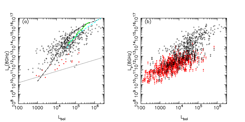
Figure 6.— Radio luminosity versus bolometric luminosity for all of the HII regions and YSOs in the catalog, (a) showing only the detections, and (b) showing all data including limits. The HII regions are crosses, the YSOs dots (colored red in the online version). Model radio luminosities are also shown in (a) after the fashion outlined in Lumsden et al. (2003). The dot-dash black line shows the results for a single star using stellar models from Lanz & Hubeny (2007), the dashed (blue in online version) line shows the results for a single star using stellar models from Pauldrach, Hoffmann & Lennon (2001), and the solid (green in online version) line the Pauldrach et al. models but for a cluster. The dotted line shows the extrapolation of jet luminosity as derived for low mass stars by Anglada (1995), as well as of the known emission from high mass stars (whether jet or wind) as given in Hoare & Franco (2007).

The detected HII regions with $L\mathrel{\raise 1.16pt\hbox{$<$}\kern-7.0pt\lower 3.06pt\hbox{{$\scriptstyle\sim$}}}5\times 10^{4}$ $\rm L_{\odot}$ all tend to show more emission than the models. Since this is a luminosity-luminosity plot, the issue cannot lie wholly with inaccurate distance. Errors in the fluxes used in estimating the bolometric luminosity are likely to move points to the left if anything, since we still rely in part on large-beam IRAS data for objects outside the MIPSGAL region. Objects can be fainter than the envelope, since optical depth, leakage of ionising photons from the nebula and over-resolved interferometric data all act to give less flux than expected. Nothing however acts to make an object brighter in the radio than anticipated. The fact the envelope is so well defined, even at low luminosity, strongly suggests this is a real effect.

Significant excess Lyman continuum flux above model predictions has been observed directly in EUV observations of the nearby stars $\epsilon$ and $\beta$ CMa (Cassinelli et al. 1995, 1996). These are B2 II and B1 II–III spectral types and hence are not on the main sequence and thus perhaps not direct analogues of the young B stars ionizing UCHII regions. However, if these young stars have not completely contracted onto the main sequence they may not be so dissimilar. The timescales for the contraction onto the main sequence after the termination of accretion are of order 10⁵ years for early B stars (Figure 2 in Davies et al. 2011), which is similar to the age of the UCHII regions themselves.

The physical reasons behind the order of magnitude excess Lyman continuum flux are still being sought. An infrared excess in the B2 II stars showed that the outer layers of the atmosphere were warmer than the models predict. Krticka, Korcakova and Kubat (2005) discuss the effects of Doppler and frictional heating of stellar winds that are significant in the cooler B stars. The hot, X-ray dominated winds in some late O star main sequence stars may also be of relevance here (Huenemoerder et al. 2012).

Finally, Figure 6(b) clearly shows that most of the detected massive YSOs lie below the HII region detections. The radio emission from these objects is not nebular. The stars simply lack ultraviolet flux (as is also evident from the near infrared spectra presented by Cooper et al. 2013). They are therefore “radio weak” compared to the HII regions with the same luminosity. This deficit of ultraviolet photons is in agreement with models for massive YSOs which predict the star swells and cools as it accretes (eg Hosokawa & Omukai 2009). Two possible alternatives then exist for the source of the radio emission. We may be seeing emission from an ionised jet (see, eg, Figure 5 in Anglada 1995, which we have fitted together with the known high mass radio detections in YSOs from Hoare & Franco (2007), to derive a relationship through the luminosity regime in Figure 6). This perhaps lies at the base of any larger scale molecular outflow. Alternatively, we may be seeing an equatorially flattened wind (eg Hoare 2006). The relative paucity of actual detections in our existing radio data, as well as their relatively modest spatial resolution, makes it impossible to distinguish between these cases.

4.2. Virialised Motions in Massive Cores?

As part of the follow-up observations for the RMS survey we have acquired a significant quantity of new mm CO line data in order to derive kinematic distances to our sources. The line intensities were not fully calibrated, but the velocities and line widths are.

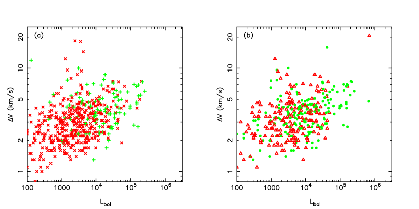
Figure 7.— Bolometric luminosity versus linewidth of our observed ¹³CO data. The sample is limited to those objects with distances nearer than 5kpc for comparison with the results of Figure 9. The data for YSOs (x, colored red in the online version) and HII regions (+, colored green in the online version) are shown in (a), and the same set of data but split by color in (b), with the points (green in the online version) having $F_{21}/F_{8}>10$ and the triangles (red in the online version) $4<F_{21}/F_{8}<10$.

In Figure 7 we plot the relationship for HII regions and YSOs between the full width at half maximum of the ¹³CO emission and the bolometric luminosity. We have curtailed the sample to those with distances within 5kpc, and limited the HII regions to those objects which appear point-like in the WISE data (see Section 2.7 for details). The left hand plot shows where HII regions and YSOs lie separately, the right hand plot shows all HII regions and YSOs, but instead shows where objects fall as a function of the $F_{21}/F_{8}$ ratio, where we have split the data into two around $F_{21}/F_{8}=10$. The more luminous objects in Figure 7 have the broader lines. The formal Pearson correlation coefficient between $\log(\Delta v)$ and $\log L$ is $\sim 0.43$ for 523 objects. Urquhart et al. (2011b) found a similar relationship using the width of the NH₃ line for an overlapping but not identical sample of YSOs and HII regions drawn from RMS.

The correlation holds separately for YSOs, with a correlation coefficient of 0.41 for 422 YSOs. By comparison the HII region sample on its own shows no significant evidence for a correlation (correlation coefficient of 0.10 for 101 HII regions), rising to 0.19 if the restriction on “point-like” HII regions is removed). It is possible that the the bulk expansion motions seen in the gas around HII regions destroys any correlation there. Not all of our YSOs show evidence for an outflow (Maud et al. in preparation), which suggests that the good correlation seen for the YSOs is actually a fundamental property of the natal molecular cloud rather than due to the energetics of the central source.

Urquhart et al. suggested that this relationship was due to the correlation between linewidth and the mass of the natal clump (ie it is essentially a virial relation, eg Larson 1981), and that seems the most natural explanation here too. Potentially, this also explains the weak color segregation present in $F_{21}/F_{8}$ as well, since we would expect the objects that will become more massive to have higher accretion rates, and hence have redder colors in the thermal infrared. High accretion rates can only be sustained if the core itself is more massive, naturally leading to redder objects having somewhat enhanced linewidths.

4.3. Galactocentric Radial Distribution of RMS Sources

The distribution of the RMS sources in the Galaxy has previously been considered by Urquhart et al. (2011a), but we are now in a position to accurately study how this varies with the type of source. In Figure 8 we show the distribution of both HII regions and YSOs as a function of Galactocentric radius. We have restricted the sample to those objects with $L_{bol}>10000$ $\rm L_{\odot}$, and distance from us of less than 10kpc to match the rough completeness limit of the catalog. A Mann-Whitney U-test suggests these differ in the sense that the YSOs lie at larger radii at the 99% confidence level. This could partly be a selection effect. It is easier to see bright radio emitting HII regions in the considerable background near the Galactic centre than it is a YSO. There is a lack of HII regions in the outer galaxy compared to the YSOs however, and this cannot be a selection effect. In part this also appears to be a luminosity effect. If we compare the YSOs against the HII regions with $L_{bol}<100000$ $\rm L_{\odot}$, the confidence level drops to 95%. This value was chosen as the approximate upper limit of YSO luminosity. By contrast the confidence level that the samples are different is $>99$% when we compare the higher luminosity HII regions with the YSOs. There is only one HII region with luminosity above this threshold beyond a Galactocentric radius of 10kpc – the other 62 all lie inwards.

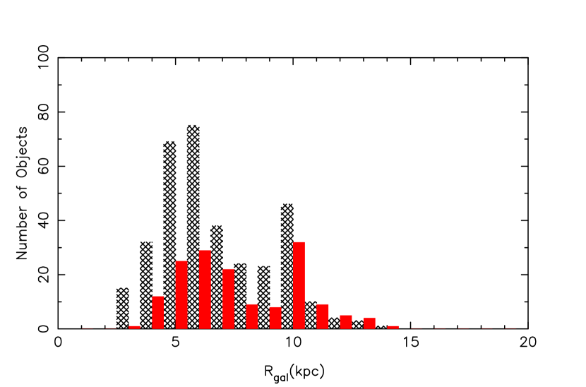
Figure 8.— Distribution of galactocentric radius for HII regions (grey hatched bars) and YSOs (solid, colored red in online version). Only sources with bolometric luminosity greater than $10^{4}\mbox{\,$\rm L_{\odot}$}$ and distance from us of less than 10kpc are included.

The most obvious explanation if this result is correct is that high mass cores are more likely in the crowded central regions. Lepine et al. (2011) have found a similar “step-change” in numbers of open clusters and the metallicity gradient at a similar Galactocentric distance of 8.5kpc. They explain it as being due to a gap in the dense gas at the co-rotation radius, that isolate properties in the inner Galactic Plane from those outside the co-rotation radius. Their explanation requires smaller gas flows outside the co-rotation radius, which will lead to less collisions between cloud cores. It seems plausible that the most massive star formation regions arise through such collisions (eg. van Loo, Falle and Hartquist 2007), giving a natural explanation for the result we see.

4.4. Color-Luminosity Relationships

Finally we consider how the colors of the YSOs and HII regions vary as a function of luminosity. Figure 9 shows data using the MSX $F_{21}/F_{8}$ ratio as well as the ratio from WISE bands 3 and 2 (12 and 4.6$\mu$m). The latter is a useful test since the beam size for these wavelengths is a factor of three smaller than for the MSX data. Again we have curtailed the sample to those sources which appear point-like in WISE at 12$\mu$m, and which lie within 5kpc. The latter is important here since we see more HII regions to greater distances due to their greater luminosity on average. The line of sight extinction, and hence to some extent the thermal infrared color, increase with distance creating a bias.

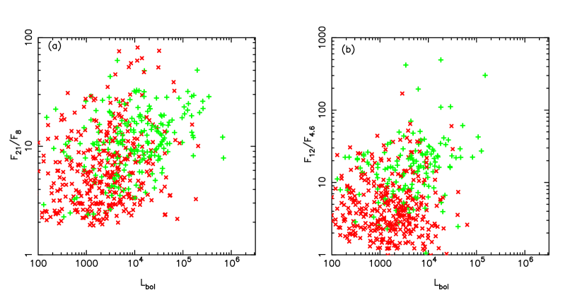
Figure 9.— Bolometric luminosity versus mid-infrared color. The left hand plot shows data from the MSX satellite, the right data from WISE. The sample is limited to those objects with distances nearer than 5kpc. The YSOs are shown as x (colored red in online version) and HII regions as + (colored green in online version). There is a clear sense in which the HII regions are redder than the YSOs on average.

The HII regions, on average, are redder than the YSOs in both ratios. This points towards a picture in which HII regions are more embedded. The only other factor that can play a part is geometry. This comes into play in two ways. Orientation is important in determining the colors of a YSO, since a more edge-on accretion disc source will suffer greater extinction than one we see pole-on. However the data shown should randomly sample all inclinations. This may give rise to the large scatter in color seen, but cannot explain the difference between the HII regions and the YSOs. The second factor is the extent of the HII region. More evolved HII regions, as they grow larger, naturally support a greater volume of Ly$\alpha$ heated dust. This should shift the colors bluewards, since there is more emission away from the centre of the natal core. Again part of the scatter could be due to this effect. Since this factor should make HII regions bluer however, it cannot explain why HII regions are actually redder than YSOs. The colors, like the virial estimates, again suggest more massive cores, which have greater line of sight reddening towards the centre of the core, give rise to higher luminosity sources.

5. Summary

The final catalog from the Red MSX Source Survey presents a comprehensive view of the infrared bright phase of the massive protostellar population of our galaxy. It is complete for objects as faint as a typical B0 star at the distance of the Galactic centre and for more luminous sources across the whole galaxy. We currently have almost 700 YSOs and HII regions with confirmed luminosities above this threshold. In addition we have identified many more YSOs that can be characterised as embedded Herbig Be stars that lie below this luminosity, providing a valuable, though incomplete, resource for the study of young intermediate mass stars as well. The combination of a bright saturation limit for the initial MSX catalog together with the coverage of the whole Galactic Plane out to $|b|<5^{\circ}$ makes it the ideal catalog for these infrared bright sources. Comparison with both older lower spatial resolution catalogs of massive young stellar objects derived from IRAS, and more recent higher spatial resolution candidates from both Spitzer and WISE, as well as high resolution radio studies, suggests that our catalog is highly reliable and complete for the massive young stellar object class. It is likely to remain the best source for this infrared bright phase for some time, given the relatively low saturation limits of the IRAC and MIPS instruments from Spitzer, and to a lesser extent for the detectors on WISE. This compromises the ability of those missions to study the most massive star formation regions and most luminous sources.

The full RMS catalog has also been used by other groups for aspects of research into massive star formation. Guzman et al. (2010, 2012) have studied the radio properties of objects they classify as “radio weak”, in a bid to detect hypercompact HII regions, jets and stellar winds. Thompson et al. (2012) examined the incidence of triggering using RMS sources around bubbles found in Spitzer data. Moore et al. (2012) studied the correlation of available gas reservoirs with our MYSOs in order to determine how star formation efficiency varies as a function of location within the spiral arms. Davies et al. (2012) used the distances we have derived to our YSOs and HII regions to help pin down the distances to massive star clusters. In addition, other groups have adopted similar color selection criteria to those present in Lumsden et al. (2002) in order to study heavily obscured evolved stars (eg. Ortiz et al 2005). Our catalog contains a large number of highly obscured evolved stars likely to be of interest to those interested in topics such as post-AGB evolution.

We have also shown that the wealth of data we have acquired can themselves identify both new properties (the excess UV flux from young intermediate mass stars), as well as provide indications as to how massive stars form. The correlation between luminosity and apparent virial mass suggests that these dynamical processes are essentially responsible for setting the initial condition rather than the ongoing formation. This tends to favour models of monolithic collapse, though competitive accretion may play an important role at an earlier phase when the clumps themselves are merging, and possibly also in feeding residual mass to the most massive star present one it has formed. The split between inner and outer galaxy may also signify the greater role that triggering and spiral density waves can play in denser environments.

Finally we note that the RMS catalog is already the basis for numerous further studies in massive star formation, such as the properties of outflows. When combined with appropriate catalogs of the initial phases of massive star evolution from other indicators (eg.  Caswell et al. 2010, Contreras et al. 2013, Molinari et al. 2010), a complete census, and understanding of the evolution, of the massive star population from initial core through to main sequence will be possible. This should provide firm answers to the remaining questions as to how massive stars form.

6. Acknowledgments

We would like to thank the referee for their comments. This work was supported by the STFC. SLL also acknowledges the support of PPARC through the award of an Advanced Research Fellowship during the early stages of this work. This publication makes use of data products from the Two Micron All Sky Survey, which is a joint project of the University of Massachusetts and the Infrared Processing and Analysis Center/California Institute of Technology, funded by the National Aeronautics and Space Administration and the National Science Foundation. This research has made use of the SIMBAD database, operated at CDS, Strasbourg, France. This work is based in part on observations made with the Spitzer Space Telescope, obtained from the NASA/ IPAC Infrared Science Archive, both of which are operated by the Jet Propulsion Laboratory, California Institute of Technology under a contract with the National Aeronautics and Space Administration. This publication makes use of data products from the Wide-field Infrared Survey Explorer, which is a joint project of the University of California, Los Angeles, and the Jet Propulsion Laboratory/California Institute of Technology, funded by the National Aeronautics and Space Administration.

References

Anglada G., 1995, RMxAC, 1, 67

Benjamin R.A., et al., 2003, PASP, 115, 953

Bonnell, I.A., Vine, S.G., Bate, M.R., 2004, MNRAS, 349, 735

Campbell B., Persson S.E., Matthews K., 1989, AJ, 98, 643

Carey S.J., et al., 2009, PASP, 121, 76

Carpenter J.M., Snell R.L., Schloerb F.P., Skrutskie M.F., 1993, ApJ, 407, 657

Casali M., et al., 2007, A&A, 467, 777

Cassinelli, J.P., et al., 1995, ApJ, 438, 932

Cassinelli, J.P., et al., 1996, ApJ, 460, 949

Caswell, J.L., Fuller, G.A., Green, J.A., et al. 2010, MNRAS, 404, 1029

Chan S.J., Henning T., Schreyer K., 1996, A&AS, 115, 285

Churchwell E., et al., 2009, PASP, 121, 213

Clarke A.J., Oudmaijer R.D., Lumsden S.L., 2005, MNRAS, 363, 1111

Contreras, Y., et al., 2013, A&A, 549, A45

Cooper H.D.B., et al., 2013, MNRAS, 430, 1125

Cutri R. M., et al., 2012, “Explanatory Supplement to the WISE All-Sky Data Release Products”

Davies B., Hoare M.G., Lumsden S.L., Hosokawa T., Oudmaijer R.D., Urquhart J.S., Mottram J.C., Stead J., 2011, MNRAS, 416, 972

Davies, B., et al., 2012, MNRAS, 419, 1871

de Wit W.J., Hoare M.G., Oudmaijer R.D., Lumsden S.L., 2010, A&A, 515, A45

Eder J., Lewis B.M., Terzian Y., 1988, ApJS, 66, 183

Egan M.P., Price S.D., Kraemer K.E., Mizuno D.R., Carey S.J., Wright C.O., Engelke C.W., Cohen M., Gugliotti G. M., 2003, The Midcourse Space Experiment Point Source Catalog Version 2.3 Explanatory Guide, Air Force Research Laboratory Technical Report AFRL-VS-TR-2003-1589

Gallaway M., et al., 2013, MNRAS, 626

Gennaro M., Brandner W., Stolte A., Henning T., 2011, MNRAS, 412, 2469

Green, J.A., Caswell, J.L., Fuller, G.A., et al. 2009, MNRAS, 392, 783

Green, J.A., McClure-Griffiths, N.M. 2011, MNRAS, 417, 2500

Green, J.A., Caswell, J.L., Fuller, G.A., et al. 2012, MNRAS, 420, 3108

Guzmán A.E., Garay G., Brooks K.J., 2010, ApJ, 725, 734

Guzmán, A.E., Garay, G., Brooks, K.J., Voronkov, M.A. 2012, ApJ, 753, 51

Hambly N.C., et al., 2008, MNRAS, 384, 637

Helfand, D.J., Becker, R.H., White, R.L., Fallon, A., Tuttle, S. 2006, AJ, 131, 2525

Hewett P.C., Warren S.J., Leggett S.K., Hodgkin S.T., 2006, MNRAS, 367, 454

Hoare, M.G., 2006, ApJ, 649, 856

Hoare M.G., Roche P.F., Glencross W.M., 1991, MNRAS, 251, 584

Hoare, M.G., Franco, J., 2007, In: “Diffuse Matter from Star Forming Regions to Active Galaxies - A Volume Honouring John Dyson”, Edited by T.W. Hartquist, J.M. Pittard, and S.A.E.G. Falle. Series: Astrophysics and Space Science Proceedings. Springer Dordrecht, 2007, p.61

Hoare M.G., et al., 2012, PASP, 124, 939

Hodapp K.-W., 1994, ApJS, 94, 615

Hodgkin S.T., Irwin M.J., Hewett P.C., Warren S.J., 2009, MNRAS, 394, 675

Hodgkin S., Irwin M., Lewis J., Gonzalez-Solares E., Yoldaş A.K., 2012, Star Clusters in the Era of Large Surveys, Astrophysics and Space Science Proceedings, Springer-Verlag, Berlin Heidelberg, p39

Hosokawa T., Omukai K., 2009, ApJ, 691, 823

Hosokawa T., Yorke H.W., Omukai K., 2010, ApJ, 721, 478

Huenemoerder, D.P., Oskinova, L.M., Ignace, R., Waldron, W.L., Todt, H., Hamaguchi, K., Kitamoto, S., 2012, ApJ, 756, L34

Kahn F.D., 1974, A&A, 37, 149

Krumholz, M.R., Klein, R.I., McKee, C.F., Offner, S.S.R., & Cunningham, A.J., 2009, Science, 323, 754

Krumholz, M.R., Cunningham, A.J., Klein, R.I., McKee, C.F., 2010, ApJ, 713, 1120

Krticka, J., Korcakova, D., Kubat J., 2005, PAICz, 93, 29

Kuiper, R., Klahr, H., Beuther, H., Henning, T., 2010, ApJ, 722, 1556

Kuiper, R., Yorke, H.W., 2013, ApJ, 763, 104

Kurtz S., Churchwell E., Wood D.O.S., 1994, ApJS, 91, 659

Lawrence A., et al., 2007, MNRAS, 379, 1599

Lanz T., Hubeny I., 2007, ApJS, 169, 83

Larson R.B., 1981, MNRAS, 194, 809

Lépine J.R.D., et al., 2011, MNRAS, 417, 698

Lewis J.R., Irwin M., Bunclark P., 2010, ASPC, 434, 91

Lucas P.W., et al., 2008, MNRAS, 391, 136

Lumsden S.L., Hoare M.G., Oudmaijer R.D., Richards D., 2002, MNRAS, 336, 621

Lumsden S.L., Puxley P.J., Hoare M.G., Moore T.J.T., Ridge N.A., 2003, MNRAS, 340, 799

McKee, C.F., Tan, J.C., 2003, ApJ, 585, 850

Martins F., Schaerer D., Hillier D.J., 2005, A&A, 436, 1049

Minniti D., et al., 2010, NewA, 15, 433

Mizuno D.R., et al., 2008, PASP, 120, 1028

Molinari S., et al., 2010, PASP, 122, 314

Moore, T.J.T., Urquhart, J.S., Morgan, L.K., Thompson, M.A. 2012, MNRAS, 426, 701

Mottram J.C., Hoare M.G., Lumsden S.L., Oudmaijer R.D., Urquhart J.S., Sheret T.L., Clarke A.J., Allsopp J., 2007, A&A, 476, 1019

Mottram J.C., Hoare M.G., Lumsden S.L., Oudmaijer R.D., Urquhart J.S., Meade M.R., Moore T.J.T., Stead J.J., 2010, A&A, 510, A89

Mottram J.C., et al., 2011a, A&A, 525, A149

Mottram J.C., et al., 2011b, ApJ, 730, L33

Ortiz, R., Lorenz-Martins, S., Maciel, W.J., & Rangel, E.M. 2005, A&A, 431, 565

Pauldrach A.W.A., Hoffmann T.L., Lennon M., 2001, A&A, 375, 161

Price S.D., Egan M.P., Carey S.J., Mizuno D.R., Kuchar T.A., 2001, AJ, 121, 2819

Purcell C.R., et al., 2013, ApJS, 205, 1

Reid M.J., et al., 2009, ApJ, 700, 137

Rygl, K.L.J., Brunthaler, A., Reid, M.J., et al. 2010, A&A, 511, A2

Schuller, F., Menten, K.M., Contreras, Y., et al. 2009, A&A, 504, 415

Shu F.H., Adams F.C., Lizano S., 1987, ARA&A, 25, 23

Skrutskie M.F. et al., 2006, AJ, 131, 1163

Sridharan T.K., Beuther H., Schilke P., Menten K.M., Wyrowski F., 2002, ApJ, 566, 931

Thompson, M.A., Urquhart, J.S., Moore, T.J.T., Morgan, L.K. 2012, MNRAS, 421, 408

Urquhart J.S., et al., 2007a, A&A, 474, 891

Urquhart J.S., Busfield A.L., Hoare M.G., Lumsden S.L., Clarke A.J., Moore T.J.T., Mottram J.C., Oudmaijer R.D., 2007b, A&A, 461, 11

Urquhart, J.S., Busfield, A.L., Hoare, M.G., et al. 2008, A&A, 487, 253

Urquhart J.S., et al., 2009, A&A, 501, 539

Urquhart J.S., et al., 2011a, MNRAS, 410, 1237

Urquhart, J.S., Morgan, L.K., Figura, C.C., et al. 2011, MNRAS, 418, 1689

Urquhart, J.S., Hoare, M.G., Lumsden, S.L., et al. 2012, MNRAS, 420, 1656

Urquhart, J.S., Moore, T.J.T., Schuller, F., et al. 2013a, MNRAS, 431, 1752

Urquhart, J.S., Thompson, M.A., Moore, T.J.T., et al. 2013b, MNRAS, in press (arXiv:1307.4105)

van Loo, S., Falle, S.A.E.G., & Hartquist, T.W. 2007, MNRAS, 376, 779

Wright E.L., et al., 2010, AJ, 140, 1868

Name	RA	Dec	$D$	$L_{bol}$	Other	Name	RA	Dec	$D$	$L_{bol}$	Other
			(kpc)	( $\rm L_{\odot}$)	Name				(kpc)	( $\rm L_{\odot}$)	Name
G010.3208-00.1570B	18:09:01.48	-20:05:08.0	3.5	41600		G010.8411-02.5919	18:19:12.10	-20:47:30.9	1.9	23700	GGD 27
G012.0260-00.0317	18:12:01.89	-18:31:55.8	11.1	24600	IRAS 18090-1832	G012.1993-00.0342B	18:12:23.43	-18:22:51.0	12.0	34700	IRAS 18094-1823
G012.9090-00.2607	18:14:39.56	-17:52:02.3	2.4	21700	W33A	G017.6380+00.1566	18:22:26.38	-13:30:12.0	2.2	53100	GL2136
G017.9789+00.2335A	18:22:49.14	-13:10:01.5	14.4	31300		G018.3412+01.7681	18:17:58.11	-12:07:24.8	2.8	21800	IRAS 18151-1208
G020.7617-00.0638B	18:29:12.11	-10:50:36.2	11.8	20800		G021.5624-00.0329	18:30:36.07	-10:07:11.1	9.7	23700
G023.3891+00.1851	18:33:14.32	-08:23:57.5	4.5	41900		G026.2020+00.2262	18:38:18.51	-05:52:57.5	7.5	30500
G027.1852-00.0812A	18:41:13.18	-05:09:01.0	13.0	94300	IRAS 18385-0512	G028.3046-00.3871A	18:44:21.97	-04:17:39.5	10.0	38500
G028.8621+00.0657	18:43:46.25	-03:35:29.3	7.4	146200	IRAS 18411-0338	G029.8620-00.0444	18:45:59.55	-02:45:06.5	7.3	56000	CH3OH 029.86-00.05
G030.1981-00.1691	18:47:03.07	-02:30:36.1	7.3	33200		G030.9585+00.0862B	18:47:31.83	-01:42:59.6	11.7	50400
G030.9727+00.5620	18:45:51.69	-01:29:13.0	12.6	22900		G032.0451+00.0589	18:49:36.56	-00:45:45.5	4.9	20400	IRAS 18470-0049
G032.9957+00.0415A	18:51:24.45	+00:04:34.1	9.2	22500	IRAS 18488+0000	G034.0126-00.2832	18:54:25.06	+00:49:56.6	12.9	33800
G034.0500-00.2977	18:54:32.30	+00:51:32.9	12.9	22500		G035.1979-00.7427	18:58:13.00	+01:40:31.2	2.2	30900	G35.2N
G037.5536+00.2008	18:59:09.95	+04:12:15.7	6.7	38000	IRAS 18566+0408	G042.0341+00.1905A	19:07:28.20	+08:10:53.3	11.1	29300
G042.0977+00.3521A	19:07:00.51	+08:18:44.1	10.9	31300	IRAS 19045+0813	G042.0977+00.3521B	19:07:00.52	+08:18:45.6	10.9	31300	IRAS 19045+0813
G042.1099-00.4466∗	19:09:53.57	+07:57:14.5	8.7	43400	IRAS 19074+0752	G043.0884-00.0109	19:10:09.55	+09:01:26.7	11.1	32900
G045.4543+00.0600B	19:14:21.27	+11:09:15.5	7.3	34900	IRAS 19120+1103	G045.4543+00.0600C	19:14:21.24	+11:09:20.2	7.3	34900	IRAS 19120+1103
G053.6185+00.0376	19:30:23.04	+18:20:26.6	7.9	20000		G060.5750-00.1861	19:45:52.50	+24:17:42.8	7.5	30100	IRAS 19437+2410
G060.8828-00.1295B∗	19:46:20.14	+24:35:29.3	2.2	21700	S87 IRS1	G062.5748+02.3875	19:40:21.52	+27:18:43.7	13.4	96100	IRAS 19383+2711
G064.8131+00.1743	19:54:05.86	+28:07:40.6	8.2	184300	IRAS 19520+2759	G073.6525+00.1944	20:16:21.96	+35:36:06.3	11.2	259200	IRAS 20144+3526
G075.6014+01.6394	20:15:48.16	+38:01:31.3	11.2	28600		G076.3829-00.6210∗	20:27:26.77	+37:22:47.8	1.4	39700	S106 IRS4
G078.7641+01.6862	20:24:51.67	+40:39:25.3	10.5	42300		G078.8867+00.7087	20:29:24.87	+40:11:19.4	3.3	185300	GL2591
G085.4102+00.0032A	20:54:14.36	+44:54:04.6	5.5	20400		G090.2095+02.0405	21:03:41.76	+49:51:47.1	7.4	29700	IRAS 21020+4939
G094.4637-00.8043	21:35:09.11	+50:53:09.6	4.9	20800	IRAS 21334+5039	G094.6028-01.7966	21:39:58.25	+50:14:20.9	4.9	43200	V645 Cyg
G096.5438+01.3592	21:35:43.82	+53:53:09.4	7.0	22600	IRAS 21340+5339	G097.5268+03.1837B	21:32:11.30	+55:53:39.9	6.9	30600
G097.5268+03.1837C	21:32:10.69	+55:53:35.4	6.9	21700	S128 IRS 2	G102.3533+03.6360	21:57:25.19	+59:21:56.7	8.4	107000	CPM 36
G110.1082+00.0473B∗	23:05:10.15	+60:14:42.8	4.3	28400	S156A	G111.2348-01.2385	23:17:21.02	+59:28:48.0	4.4	41900	IRAS 23151+5912
G111.2824-00.6639B	23:16:03.85	+60:01:56.8	3.5	24700	IRAS 23138+5945	G111.5671+00.7517	23:14:01.76	+61:27:19.9	2.7	44600	NGC 7538 IRS 9
G133.6945+01.2166A	02:25:30.99	+62:06:21.0	2.0	28500	W3 IRS4 (part)	G133.7150+01.2155	02:25:40.78	+62:05:52.5	2.0	206300	W3 IRS5
G135.2774+02.7981	02:43:28.65	+62:57:08.7	6.0	28500	IRAS 02395+6244	G151.6120-00.4575	04:10:11.86	+50:59:54.5	6.4	21500	CPM 12
G192.6005-00.0479	06:12:54.01	+17:59:23.1	2.0	35600	S255 IRS1	G196.4542-01.6777	06:14:37.06	+13:49:36.5	5.3	94000	IRAS 06117+1350
G269.8539-00.0630	09:11:08.34	-48:15:56.3	8.4	27600		G274.0649-01.1460A	09:24:42.55	-52:01:50.6	5.7	24300
G281.0472-01.5432	09:59:15.88	-56:54:39.3	7.0	145100		G281.7578-02.0132	10:01:21.58	-57:42:56.4	7.0	32300
G282.0598-00.5721	10:09:26.56	-56:43:49.5	4.9	20000		G282.8969-01.2727	10:11:31.60	-57:47:03.7	7.0	31900
G289.9446-00.8909A	11:01:10.67	-60:57:08.4	8.3	26200		G299.5265+00.1478	12:21:50.64	-62:31:42.4	7.5	34700
G300.5047-00.1745A	12:30:03.60	-62:56:48.4	8.9	42700		G301.8147+00.7808A	12:41:53.87	-62:04:14.6	4.4	22000	IRAS 12389-6147
G303.9973+00.2800∗	13:00:41.62	-62:34:20.8	11.4	20400		G304.3674-00.3359A	13:04:09.87	-63:10:20.1	11.8	88200
G304.6668-00.9654∗	13:07:08.37	-63:47:02.8	11.4	24800		G305.2017+00.2072A	13:11:10.45	-62:34:38.6	4.0	30300	CH3OH 305.20+00.21
G305.3676+00.2095	13:12:36.49	-62:33:32.3	4.0	28100		G305.5610+00.0124	13:14:26.37	-62:44:30.5	4.0	42000
G308.9176+00.1231A	13:43:01.70	-62:08:51.2	5.3	186800	OH 308.918+00.123	G309.9206+00.4790B	13:50:42.34	-61:35:07.9	5.4	26600	IRAS 13471-6120
G310.0135+00.3892	13:51:37.86	-61:39:07.5	3.2	54600	IRAS 13481-6124	G319.3993-00.0135C	15:03:17.68	-58:36:14.8	11.7	109800
G319.8366-00.1963	15:06:54.49	-58:32:58.8	11.7	38900		G321.0523-00.5070	15:16:06.11	-58:11:41.8	9.1	74400
G321.3824-00.2861	15:17:20.21	-57:50:00.3	9.4	24600		G327.1192+00.5103	15:47:32.81	-53:52:39.4	4.9	41600	CH3OH 327.120+00.511
G328.2523-00.5320A	15:57:59.83	-53:58:00.5	2.9	40500	CH3OH 328.25-00.53	G328.2523-00.5320B	15:57:59.38	-53:57:57.4	2.9	21300
G329.0663-00.3081	16:01:09.93	-53:16:02.3	11.6	65600	CH3OH 329.07-00.31	G331.2759-00.1891B	16:11:26.00	-51:41:57.0	4.9	35000	CH3OH 331.278-00.188
G331.3576+01.0626	16:06:25.78	-50:43:22.0	4.5	22200	IRAS 16026-5035	G331.5131-00.1020	16:12:09.96	-51:28:37.1	5.0	69300	OH 331.512-00.103
G331.5180-00.0947A	16:12:08.95	-51:28:02.3	5.0	32100		G331.7953-00.0979	16:13:28.04	-51:16:46.8	14.5	105300
G332.0939-00.4206	16:16:16.47	-51:18:25.2	3.6	76100		G332.8256-00.5498A∗	16:20:11.07	-50:53:16.2	3.6	207700
G332.9868-00.4871	16:20:37.81	-50:43:49.7	3.6	26700		G333.1256-00.4367	16:21:02.66	-50:35:55.4	3.6	85000	CH3OH 333.126-00.440
G334.8438+00.2095A	16:25:40.51	-48:55:16.2	10.6	25400		G336.8308-00.3752	16:36:26.16	-47:52:30.9	13.5	50900
G338.0008-00.1498A	16:40:04.02	-46:51:18.1	11.4	50400		G338.2253-00.5094	16:42:30.98	-46:55:22.6	13.7	103000
G338.3597+00.1430A	16:40:11.88	-46:23:27.2	12.8	30100		G338.4712+00.2871	16:39:58.91	-46:12:36.5	13.1	86100	IRAS 16363-4606
G338.4763+00.0418A	16:41:04.46	-46:22:18.8	12.6	28200		G338.9196+00.5495	16:40:34.05	-45:42:08.0	4.2	32000
G339.3316+00.0964	16:44:04.39	-45:41:27.2	13.1	39600		G339.6221-00.1209	16:46:06.00	-45:36:43.9	2.8	23800
G339.8838-01.2588	16:52:04.66	-46:08:33.6	2.7	63900	IRAS 16484-4603	G339.9489-00.5401	16:49:07.95	-45:37:58.8	10.5	20800	EGO G339.95-0.54
G342.9583-00.3180	16:58:48.56	-43:09:32.5	12.7	62200		G343.1261-00.0623	16:58:17.21	-42:52:07.1	2.8	66100	IRAS 16547-4247
G344.4257+00.0451C	17:02:08.62	-41:47:10.2	4.7	23100		G344.6608+00.3401	17:01:41.02	-41:24:48.1	12.7	20300
G345.4938+01.4677	16:59:41.61	-40:03:43.4	2.4	154400	IRAS 16562-3959	G345.5043+00.3480	17:04:22.87	-40:44:23.5	2.0	23700	CH3OH 345.50+00.35
G349.7215+00.1203A	17:18:11.22	-37:28:24.6	11.3	65900

Table 2Complete list of the massive protostars with $L>20000$ $\rm L_{\odot}$. Objects marked with a superscript $*$ are also the central stars of HII regions.