Spectral compression of single photons

Abstract - Photons are critical to quantum technologies since they can be used for virtually all quantum information tasks: in quantum metrology higgins2007entanglement , as the information carrier in photonic quantum computation kok2007loq ; aspuru2012photonic , as a mediator in hybrid systems wallquist2009hybrid , and to establish long distance networks duan2001long . The physical characteristics of photons in these applications differ drastically; spectral bandwidths span 12 orders of magnitude from 50 THz sergienko_broadband for quantum-optical coherence tomography QOCT_Th to 50 Hz for certain quantum memories tittel2010photon . Combining these technologies requires coherent interfaces that reversibly map centre frequencies and bandwidths of photons to avoid excessive loss. Here we demonstrate bandwidth compression of single photons by a factor 40 and tunability over a range 70 times that bandwidth via sum-frequency generation with chirped laser pulses. This constitutes a time-to-frequency interface for light capable of converting time-bin to colour entanglement Pol_to_Color_Ramelow2009 and enables ultrafast timing measurements. It is a step toward arbitrary waveform generation kielpinski for single and entangled photons.

Coherent photonic interfaces are paramount for future quantum technologies. In quantum networks duan2001long for example, photon pairs at 1550 nm—optimum for low-loss transmission—distribute entanglement between network nodes consisting of quantum memories. Parametric downconversion (SPDC) sources are widespread for producing entangled photon pairs review_SinglePhoton , and typically yield spectral bandwidths of 300 GHz. The most efficient quantum memories hosseini2011high however typically operate in the near visible wavelength regime near 800 nm with narrower bandwidths on the order of 10 MHz. This dilemma has partly been addressed through centre-frequency conversion Upconversion_Huang1992 of single photons using nonlinear optical processes in crystals  Upconversion_Kwiat2003 ; Upconversion_Gisin2005 ; langrock2005highly ; ramelow2012pec ; rakher2011_modulationDot , photonic crystal fibres FWM_McGuinness2010 and Rubidium vapor FWM_Dudin2010 . This conversion process can be highly efficient langrock2005highly ; pelc1 and can conserve quantum coherence  Upconversion_Huang1992 ; Upconversion_Gisin2005 ; FWM_Dudin2010 ; ramelow2012pec ; rakher2011_modulationDot ; FWM_McGuinness2010 . Some quantum memory schemes memory2 offer very limited control over the spectrum of reemitted photons through varying parameters of the control laser shaped_EIT .

Nonlinear optics has much more potential for manipulating and controlling the spectrum of single photons. Sum-frequency generation (SFG) is a nonlinear optical process in which a pair of optical fields of frequencies $\nu_{1}$ and $\nu_{2}$ create a third field with frequency $\nu_{3}=\nu_{1}+\nu_{2}$ Boyd . When the driving fields are transform-limited laser pulses and the acceptance bandwidth of the material is sufficiently large, the bandwidth of the SFG is larger than that of the input fields. Repeating this process with shaped, rather than transform-limited pulses, can drastically alter the spectrum of the SFG signal. Specifically, oppositely-chirped laser pulses in SFG and equally-chirped laser pulses in difference-frequency generation lead to narrow output spectra  BC_oppositechirp_1 ; BC_oppositechirp_2 ; BC_DFM_1 . It was recently proposed theoretically to employ SFG between a chirped classical pulse and a single photon to enable compression of the photon pulse in time kielpinski ; interaction of a short laser pulse with the emission from a quantum dot achieves rakher2011_modulationDot similar results through temporal gating. In this letter, we exploit pulse chirping of a classical laser and a single photon to compress the bandwidth of the single photon, from 1740 GHz to 43 GHz, which is nearing the bandwidth regime of some quantum memories memory1 ; walmsley1 . When combined with shaped pulses, nonlinear optics in the quantum regime promises a new level of control over single photons kielpinski ; Silberhorn2011 .

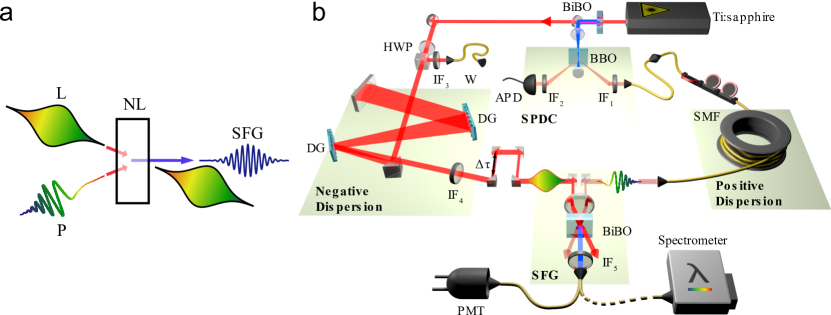
Figure 1: Single-photon bandwidth compression scheme. a, A broad-bandwidth single photon (P) with a linear frequency chirp is converted into a narrow-band photon of a higher frequency via sum-frequency generation (SFG) with a strong laser pulse (L) of opposite chirp, in a nonlinear crystal (NL). b, Experimental setup. The photon P is generated via spontaneous parametric down-conversion (SPDC) in a $\beta$-Barium-Borate (BBO) crystal (Type-I, 1 mm) and sent through 34 m of optical fiber (SMF) to introduce a linear chirp via group velocity dispersion Diels_Ultrashort . The strong laser pulse is anti-chirped after a double-pass between two diffraction gratings (DG, 1200 lines/mm) Diels_Ultrashort . The spectrally narrowed photon is generated in a 1 mm thick Bismuth-Borate (BiBO) crystal and detected with a photomultiplier tube (PMT) or sent to a spectrometer. For alignment purposes, the single photons can be substituted by a weak coherent state (W), split off from the laser beam using a half-wave plate and a polarizing beam-splitter.

Our scheme, depicted in Fig. 1(a), uses SFG between a chirped single photon and an oppositely chirped intense laser pulse. The photon is chirped such that its frequency, centered at $\nu_{0,P}$, increases in time, while the strong pulse centred at $\nu_{0,L}$ is anti-chirped such that its frequency decreases linearly in time. When the photon and pulse arrive at the crystal simultaneously, a red-shifted frequency component ($\nu_{0,P}-\delta$) will meet a blue-shifted component ($\nu_{0,L}+\delta$) with the same detuning $\delta$ and as a consequence, all frequency components will sum to a narrow frequency centered on $\nu_{0,SFG}=\nu_{0,P}+\nu_{0,L}$.

A light pulse can be described by the frequency-dependent electric field, $E(\nu)=U(\nu)e^{i\phi(\nu)}$, where $U(\nu)$ and $\phi(\nu)$ define the amplitude and phase, respectively. A linear chirp results when a transform-limited pulse is subject to a quadratic phase, $\phi(\nu)\sim A(\nu-\nu_{0})^{2}$, with $\nu_{0}$ the central frequency and $A$ is a constant. A chirp increases the pulse duration and causes its instantaneous frequency to vary linearly in time $\nu(t)=\frac{d\phi(t)}{dt}=\nu_{0}\pm 2\pi\frac{1}{2A}t$. When the chirped single photon (P) and anti-chirped strong laser pulse (L) have a relative time delay at the nonlinear crystal, $\Delta\tau$, the expected upconverted frequency is

$$\nu_{0,SFG}(\tau)=\nu_{0,P}+\nu_{0,L}+2\pi\frac{1}{2A}\Delta\tau,$$ (1)

where we assume the pulses have equal and opposite chirp, $\pm A$. We consider the large chirp limit, where each pulse is stretched many times its transform-limited duration, i.e., $A^{2}\Delta\nu^{4}\gg 1$, where $\Delta\nu$ is the full width at half-maximum (FWHM) of the spectral intensity distribution. We show in the Supplementary Material that the expected intensity bandwidth (FWHM) of the upconverted single photon is

$$\Delta\nu_{SFG}^{TH}\approx\frac{\ln{4}}{A}\sqrt{\frac{1}{\Delta\nu_{P}^{2}}+\frac{1}{\Delta\nu_{L}^{2}}}.$$ (2)

Our technique thus compresses the spectral bandwidth of the photon by a factor inversely proportional to the chirp parameter $A$. By adjusting the delay between the pulses, the central frequency $\nu_{0,SFG}(\tau)$ of the upconverted photons can be tuned over some frequency range, approximately $\sqrt{\Delta\nu_{P}^{2}+\Delta\nu_{L}^{2}}$ (see Supplementary Information), limited by the spectra of the initial single photon and laser pulse.

The experimental setup is shown in Fig. 1(b); more details are in the Methods. The second harmonic of a pulsed laser is used to produce non-degenerate signal and idler photons through down-conversion, while the remainder of the fundamental serves as the strong classical pulse. We first measure the spectrum of the signal photons at the source, after the interference filter IF₁, using a fiber-coupled spectrometer and find a width $\Delta\nu_{P}=1740\pm 50$ GHz FWHM centered around $811.11\pm 0.01$ nm, see Fig. 2. The photons are then sent through an optical fiber with positive dispersion and superposed with the anti-chirped strong laser pulse ($\Delta\nu_{L}=4770\pm 20$ GHz) centered at $787.62\pm 0.02$ nm) at the nonlinear crystal for sum-frequency generation.

The upconverted light is coupled into a single-mode fiber and sent to the spectrometer. As shown in Fig. 2, we observe significant spectral compression. The measured bandwidth is $\Delta\nu_{M}=74\pm 4$ GHz centered at 399.7 nm. Taking the resolution of our spectrometer into account, $\Delta\nu_{R}=60\pm 4$ GHz (FWHM), the actual width of the upconverted photon after deconvolution is $\Delta\nu_{SFG}^{EXP}=\sqrt{\Delta\nu_{M}^{2}-\Delta\nu_{R}^{2}}=43\pm 9$ GHz (see Supplementary Information for more details). This agrees closely with theory, $\Delta\nu_{SFG}^{TH}=32.9\pm 0.9$ GHz from equation (2), using the expected chirp parameter $A=(-25.8\pm 0.3)\times 10^{6}$ fs² given by the geometry of our grating-based stretcher. We have therefore achieved a compression ratio of 40:1 in the single photon frequency bandwidth. Similar measurements were made after replacing the single photons by a weak coherent state (W), shown in Fig. 1(b). The corresponding measured spectral width of the upconverted light was $67\pm 4$ GHz, or $30\pm 12$ GHz after deconvolution, showing similar performance with a classical chirped pulse with the same characteristics as the signal photons.

Figure 2 shows the spectrum predicted by theory which would result from upconversion of the signal photon using the same pump laser without any chirp. The conversion in this case actually broadens the spectral bandwidth of the original photon by a factor of 3, increasing the bandwidth gap between flying broadband photons and narrowband quantum memories, which further highlights the importance of our scheme.

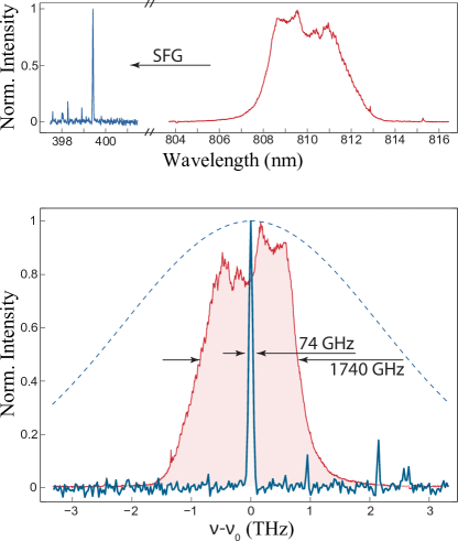
Figure 2: Single-photon spectra in wavelength (top) and relative frequency (bottom). The signal photons at the source (shown in red) have an initial bandwidth of 1740 GHz centred at 811 nm after transmission through an interference filter. Once the quadratic phase is applied and the photons are upconverted, the photon bandwidth reduces to $74\pm 4$ GHz centred at 399.70 nm (blue curve). The spectra are shown as normalised spectral intensities and for the upconverted signal case, correspond to the average of six consecutive scans of $20$ minutes acquisition time. We subtracted background counts determined by a supplementary scan with the signal photon path blocked. The blue dashed curve shows the theoretical spectrum of photons upconverted without our chirping technique but otherwise identical conditions.

The central wavelength of the narrowband upconverted photons can be tuned by controlling the relative delay $\Delta\tau$ between the photon and the laser pulse, see equation (1). The SFG spectrum was measured as a function of the delay of the single photon, with fitted central wavelengths shown in Fig. 3. The data shows that the wavelength depends linearly on the delay as expected. The linear fit gives a slope of $-0.0640\pm 0.0005$ nm/ps in good agreement with $-0.0648\pm 0.0008$ predicted from equation (1) and $A=(-25.8\pm 0.3)\times 10^{6}$ fs². If the weak coherent state is used instead of single photons, we observe the same behaviour in the spectrum of the upconverted light, and the data are also shown in Fig. 3. The lower SFG signal for single photons required longer integration times than for the coherent states; to reduce the effects of drift in experimental parameters all of the data in Fig. 3 was taken within a day. For the single photons, we focused on those delays demonstrating the widest possible tuning range. From the slope, we can extract the chirp parameter of $A=(26.2\pm 0.2)\times 10^{6}$ fs², in agreement with expectations based on the parameters of the stretcher.

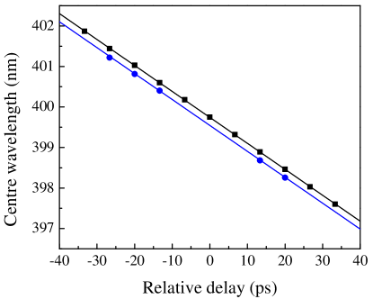
Figure 3: Wavelength tunability. The center wavelength of the upconverted light can be tuned by controling the relative delay between the input pulses at the nonlinear crystal. The blue circles represent the central wavelength of the upconverted single photon, covering a range of 3 nm. The upconverted light from the weak coherent state behaves the same way and is plotted with the black squares. The lines are linear fits yielding slopes of $-0.0640\pm 0.0005$ nm/ps and $-0.0641\pm 0.0001$ nm/ps for the single photons and the weak pulses, respectively. The vertical offset between the two curves ($\sim 0.2$ nm) comes from a slight difference in the delay between the weak coherent state and the single photons at the crystal and a difference in their central wavelength. The error bars are smaller than the data points.

Photons from SPDC are created in pairs and are strongly correlated in time; we expect these correlations are preserved through spectral compression. We first measured coincidence counts between single photon detectors placed in the source as a function of a time delay between the counts. Figure 4(a) shows the coincidence counts versus delay, without background substraction. The peak around zero delay corresponds to a rate of 160,000 s^-1, within a 3 ns coincidence window. The histogram also contains side peaks from accidental coincidences with a separation of 12.5 ns matching the laser repetition rate. After propagating through the single-mode fibre, the signal photons are upconverted and detected with a single-photon counting photomultiplier (PMT). Figure 4(b) clearly shows that the coincidence rate observed at zero-delay between the upconverted and idler photons exceed the accidentals, preserving the strong timing correlation associated with individual photon pairs. If we instead upconvert the weak coherent state, which shares the spectral and temporal properties of the signal photon, all observed peaks in Fig. 4(c) have the same height, as expected for a pulsed, but temporally uncorrelated source.

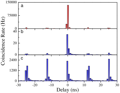
Figure 4: Temporal correlations with the idler photon. a, The signal and idler from SPDC are produced in pairs, strongly correlated in time with a total measured coincidence rate of $160,000$ s^-1 around zero delay. b, The upconverted single photon maintains the strong timing correlation expected from individual photon pairs, and a coincidence rate of 50 s^-1 is detected. c, If the weak coherent state is upconverted instead, the histogram shows equal height peaks as expected for pulsed, but uncorrelated events. For each histogram, the optical path length difference with the idler is accounted for in post-processing and the abscissa is a variable electronic delay. An additional electronic delay box, with an observed asymmetric temporal jitter, was used on the idler side only, causing the asymmetry in b) and c). Error bars, 1 s.d. too small for this scale.

The efficiency of the upconversion process in our experiment is $0.06\%$ with 300 mW of average power for the strong beam. Dramatically higher efficiencies can be achieved with the use of periodically poled crystals and higher pump powers  langrock2005highly ; pelc1 . The technique here can, in principle, reach high efficiency; however higher laser power will be required for increased compression. One doesn’t require $100\%$ conversion efficiency to achieve a net gain. Ignoring the shift in centre frequency, one has an advantage once the efficiency is greater than about $100\%/R$, where $R$ is the ratio of the initial to final bandwidth, which in our case is 40, for an efficiency of just $2.5\%$. The amount of negative dispersion achievable limits the maximum compression; with achievable parameters soyoBaek2009 and our spectra, one could achieve compression down to $\sim$1 GHz.

Future work will explore the case when the single photon is entangled with another. It is expected that polarization entanglement could be preserved by employing polarization-insensitive upconversion  ramelow2012pec . Theoretical calculations show that energy-time entanglement dramatically impacts this phenomenon (see Supplementary Information). Our technique could serve as a coherent interface between time-bin and frequency encodings of quantum information due to the delay-dependent central frequency, allowing the conversion of time-bin entanglement to colour entanglement Pol_to_Color_Ramelow2009 . It also enables ultrafast timing measurements with slow detectors review_SinglePhoton by converting different pulse arrival times to different frequencies which could more easily be distinguished. With our experimental parameters, one could distinguish time bins with separation as short as 0.6 ps over a 40 ps range. Future work will investigate nonlinear interactions with more complex shaped pulses for manipulating single photons; for example, coherent superpositions of chirped pulses with different delays would allow ultrafast single-photon time-bin measurements. The application of shaped pulse nonlinear optics is a promising and unexplored regime at the quantum level.

Methods

Our laser (Spectra Physics Tsunami HP) has a 790 nm central wavelength, 10.5 nm spectral bandwidth (FWHM), 80 MHz repetition rate, and 2.5 W average power. The laser repetition rate is stabilized by a feedback system (Lok-to-clock) which is important for the present experiment (see Supplementary Information). Second-harmonic generation in a $2$ mm thick BiBO crystal yields a beam of $830$ mW, centred at $394.2$ nm with 1.3 nm bandwidth, which generates the broadband and non-collinear photon pairs. In the signal-photon path, the interference filter IF₁ shown in Fig 1(b), with a nominal bandwidth of 5 nm (FWHM) centered around 811 nm, is inserted to keep its central frequency separated from that of the laser beam at 790 nm, to separate the spectrum of the second-harmonic background from our signal. Due to the energy conservation of SPDC, an interference filter, IF₂, centered around 770 nm and nominal bandwidth of 3 nm is inserted in the path of the idler-photon.

We first optimize the setup with a weak coherent state (W), split off from the strong laser pulse using a half-wave plate and a polarizing beam-splitter. An interference filter (IF₃) is inserted in its path and the transmitted spectrum has a measured bandwidth of $3.85\pm 0.03$ nm ($\Delta\nu_{W}=1760\pm 10$ GHz) centered at $810.49\pm 0.01$ nm, closely matched to IF₁.

The strong laser pulse was re-collimated before being anti-chirped in a grating-based setup Treacy_compressor , with normal separation of 38 cm between the gratings, carefully adjusted to minimize the spectral width of the upconverted light. The bandpass filter IF₄ highly attenuates any power in the tail of the laser spectrum above 800 nm to further suppress second-harmonic background and after the filter, the pulse has a measured bandwidth of $9.86\pm 0.05$ nm ($\Delta\nu_{L}=4770\pm 20$ GHz) centered at $787.62\pm 0.02$ nm. We used an achromatic doublet with a 75 mm focal length in the upconversion setup, and the conversion efficiency was optimized by fine tuning the relative delay between the two inputs, the spatial overlap at the crystal, and the phase matching by angle tuning. A 14.5 nm bandpass filter IF₅ with central wavelength at 405 nm is placed in the SFG beam to reduce background.

The weak beam is finally replaced by the single photons, with the same optical path length. We used a spectrometer (Acton SP-2750A) with a 1200 lines/mm diffraction gratings blazed for 400 nm and entrance opening of 20$\mu$m with a resolution of 60 GHz. We use the spectrograph, free-running mode with a back-illuminated CCD camera (PIXIS: 2048B).

S.1 SUPPLEMENTARY MATERIAL

S.2 THEORY

We model the creation of upconverted single photons through the interaction Hamiltonian, $H$, of a three-wave $\chi^{(2)}$ non-linear process. We assume that frequency bandwidths are narrow and perfect phasematching ($\vec{k}_{P}+\vec{k}_{L}-\vec{k}_{SFG}=0$) is achieved, allowing us to simplify our Hamiltonian (ignoring constants) to

$$H\propto\iiint\mathrm{d}\nu_{1}\mathrm{d}\nu_{2}\mathrm{d}\nu_{3}\hat{a}^{(P)}_{\nu_{1}}\hat{a}^{(L)}_{\nu_{2}}\hat{a}^{{\dagger}(SFG)}_{\nu_{3}}\delta(\nu_{1}+\nu_{2}-\nu_{3})+h.c.$$ (1)

Our initial three-mode state $|\psi_{i}\rangle$ is defined as a single photon $|1\rangle_{P}=\int d\nu_{1}f_{P}(\nu_{1})e^{i\phi_{P}(\nu_{1})}|1_{\nu_{1}}\rangle$, a strong coherent state $|\alpha\rangle_{L}=\int d\nu_{2}f_{L}(\nu_{2})e^{i\phi_{L}(\nu_{2})}|\alpha_{\nu_{2}}\rangle$ and an output signal, initially vacuum $|0\rangle_{SFG}$. For each of the input pulses, the frequency distribution of the field amplitude is assumed to be Gaussian, $f_{i}(\nu_{i})\propto\exp\left[-2\ln{2}\frac{(\nu_{i}-\nu_{0,i})^{2}}{\Delta\nu_{i}^{2}}\right]$, with intensity full-width at half-maximum (FWHM) $\Delta\nu_{i}$ and the phase term to contain only linear and quadratic terms $\phi_{i}(\nu_{i})=2\pi(\nu_{i}-\nu_{0,i})\tau_{i}+A_{i}(\nu_{i}-\nu_{0,i})^{2}$, where $\tau$ corresponds physically to a time delay and $A$ to a linear chirp.

Assuming no frequency correlations between the single photons and idler, a lossless and nondispersive medium, and an interaction time much longer than optical frequencies, the first order term of the time evolution of the state (postselecting on the generation of a photon in the output mode) is found to be proportional to

$$\begin{array}[]{l}|\psi^{(2)}_{f}\rangle\propto\\ \iint d\nu_{3}d\nu_{1}f_{P}(\nu_{1})f_{L}(\nu_{3}-\nu_{1})e^{i\left(\phi_{P}(\nu_{1})+\phi_{L}(\nu_{3}-\nu_{1})\right)}|1_{\nu_{3}}\rangle.\end{array}$$ (2)

From this, the electric field amplitude $E(\nu_{3})$ as a function of frequency is thus proportional to

$$E(\nu_{3})\propto\int d\nu_{1}f_{P}(\nu_{1})f_{L}(\nu_{3}-\nu_{1})e^{i\left(\phi_{P}(\nu_{1})+\phi_{L}(\nu_{3}-\nu_{1})\right)},$$ (3)

which is the convolution of the frequency domain representation of the two input pulses. Classically, assuming narrow bandwidth, the field produced in sum-frequency generation is directly proportional to the product of the two input fields in the time domain, or the convolution of the fields in the frequency domain Boyd . Thus, the same spectral properties are expected if both inputs are classical coherent states.

The field intensity $|E(\nu_{3})|^{2}$ of the upconverted photons is found to have a spectral FWHM $\Delta\nu_{SFG}$ independent of time delay $\Delta\tau$,

$$\begin{array}[]{l}\Delta\nu_{SFG}=\\ \sqrt{\frac{(A_{L}+A_{P})^{2}\Delta\nu_{L}^{4}\Delta\nu_{P}^{4}+4\ln{4}(\Delta\nu_{L}^{2}+\Delta\nu_{P}^{2})^{2}}{(A_{L}^{2}\Delta\nu_{L}^{2}+A_{P}^{2}\Delta\nu_{P}^{2})\Delta\nu_{L}^{2}\Delta\nu_{P}^{2}+4\ln{4}(\Delta\nu_{L}^{2}+\Delta\nu_{P}^{2})}}.\end{array}$$ (4)

In the case where no chirp is applied to the pulses, i.e. $A_{P}=A_{L}=0$, the bandwidth directly simplifies to $\sqrt{\Delta\nu_{P}^{2}+\Delta\nu_{L}^{2}}$. On the other hand, this bandwidth is minimized for equal and opposite chirps $A_{P}=-A_{L}=A$. If we also make the large chirp approximation that $A^{2}\Delta\nu^{4}\gg 1$, the intensity width simplifies to

$$\Delta\nu_{SFG}\approx\frac{\ln{4}}{A}\sqrt{\left(\frac{1}{\Delta\nu_{P}^{2}}+\frac{1}{\Delta\nu_{L}^{2}}\right)},$$ (5)

showing that the bandwidth is inversely proportional to the chirp rate. For our experimental parameters, $A^{2}\Delta\nu^{4}=6000$ and the approximation affects the expected frequency bandwidth by only 0.002%.

The time delay $\Delta\tau$ appears as a shift in the central frequency $\nu_{0,SFG}$ as well as an overall amplitude reduction, but has no fundamental effect on the bandwidth of the signal. Making the same assumptions as before, the central frequency $\nu_{0,SFG}$ is found to be a function of relative delay $\Delta\tau\equiv\tau_{2}-\tau_{1}$ as

$$\nu_{0,SFG}(\tau)=\nu_{0,P}+\nu_{0,L}+\frac{\pi}{A}\Delta\tau.$$ (6)

The efficiency of the upconversion process will depend on the overlap of the two pulses. If we define the frequency shift in equation (6) as $\delta\nu=\frac{\pi\Delta\tau}{A}$, the intensity of the upconverted light contains a constant prefactor reflecting the overlap, $\exp\left[-\frac{4\ln{2}\delta\nu^{2}}{\Delta\nu_{P}^{2}+\Delta\nu_{L}^{2}}\right]$. This prefactor limits the frequency tuning range to $\sqrt{\Delta\nu_{P}^{2}+\Delta\nu_{L}^{2}}$ FWHM.

Converting to wavelength as in Fig. 3 in the main text and expanding to a first-order Taylor series about zero delay, the linear wavelength shift with delay $\Delta\tau$ is found to be

$$\lambda_{0,SFG}= \frac{cA\lambda_{0,P}\lambda_{0,P}}{cA(\lambda_{0,P}+\lambda_{0,L})+\Delta\tau\pi\lambda_{0,L}\lambda_{0,P}}$$ (7)

$$\approx \frac{\lambda_{0,L}\lambda_{0,P}}{\lambda_{0,P}+\lambda_{0,P}}-\frac{\pi\lambda_{0,P}^{2}\lambda_{0,P}^{2}}{cA(\lambda_{0,L}+\lambda_{0,P})^{2}}\Delta\tau.$$ (8)

S.3 Effect of energy-time entanglement on bandwidth compression

Spontaneous parametric down-conversion often emits photons with varying degrees of energy-time entanglement, depending on the phase-matching and pump characteristics. Thus, it is important to consider the effect of our compression scheme when the single photon is part of an energy-time entangled pair. As we show in the following calculations, the presence of energy-time entanglement significantly alters the achievable bandwidth compression with our scheme.

We assume that the photon of interest, the signal ($s$), is potentially entangled with a second photon, the idler ($i$), with a combined state of the form

$$|\psi_{0}\rangle\propto\iint\mathrm{d}\nu_{s}\mathrm{d}\nu_{i}f_{P}(\nu_{s},\nu_{i})|1_{\nu_{s}}\rangle|1_{\nu_{i}}\rangle|0\rangle$$ (9)

where $f_{P}(\nu_{s},\nu_{i})$ is the joint spectral amplitude and may be inseparable. Note that we implicitly assume a single spatial and polarizaton mode for each photon, and vacuum in a third SFG mode.

We consider a linear chirp $e^{iA(\nu_{s}-\nu_{0})^{2}}$ applied to the signal photon and use the Hamiltonian of equation (1) to calculate the sum-frequency generated by a nonlinear interaction with some anti-chirped strong laser pulse ($L$), whose spectral amplitude is $\alpha(\nu_{2})=f_{L}(\nu_{2})e^{i\phi_{L}(\nu_{2})}$. Using first-order perturbation theory and only considering cases where a photon is created in the SFG mode, we have the state

$$|\psi_{f}\rangle\\ \propto\iiint\mathrm{d}\nu_{s}\mathrm{d}\nu_{i}\mathrm{d}\nu_{\scriptscriptstyle SFG}F(\nu_{s},\nu_{i},\nu_{\scriptscriptstyle SFG})|0\rangle|1_{\nu_{i}}\rangle|1_{\nu_{\scriptscriptstyle SFG}}\rangle$$ (10)

where $F(\nu_{s},\nu_{i},\nu_{\scriptscriptstyle SFG})=f_{P}(\nu_{s},\nu_{i})e^{iA(\nu_{s}-\nu_{0})^{2}}\alpha(\nu_{\scriptscriptstyle SFG}-\nu_{s})$. To find the spectral distribution of the upconverted photon, we trace out the idler photon, leaving

$$S(\nu_{\scriptscriptstyle SFG})\\ \propto\iiint\mathrm{d}\nu_{s}\mathrm{d}\nu_{s}^{\prime}\mathrm{d}\nu_{i}F^{\ast}(\nu_{s}^{\prime},\nu_{i},\nu_{\scriptscriptstyle SFG})F(\nu_{s},\nu_{i},\nu_{\scriptscriptstyle SFG}).$$ (11)

To obtain some physical intuition, we employ the model two-photon spectral function

$$f_{P}(\nu_{s},\nu_{i})\propto e^{-\frac{(\nu_{s}-\nu_{0})^{2}}{2\sigma^{2}}}e^{-\frac{(\nu_{i}-\nu_{0})^{2}}{2\sigma^{2}}}e^{-\frac{(\nu_{s}+\nu_{i}-2\nu_{0})^{2}}{2\sigma_{c}^{2}}}$$ (12)

where $\sigma$ is related to the bandwidth of each photon. The constant $\sigma_{c}$, controls the degree of entanglement in the system. In the limit where $\sigma_{c}\rightarrow\infty$, the correlation term is constant and the spectral function is separable. In the opposite limit, where $\sigma_{c}\rightarrow 0$, the correlation term becomes a delta function $\delta(2\nu_{0}-\nu_{s}-\nu_{i})$ and the two photons are perfectly energy-time entangled. For simplicity, we have assumed the photons are degenerate, where the central frequencies of the signal and idler photons are equal. Note that the intensity spectral bandwidth of one of the photons is $\Delta\nu_{P}=2\sqrt{\ln{2}}\sqrt{\frac{\sigma^{2}(\sigma_{c}^{2}+\sigma^{2})}{\sigma_{c}^{2}+2\sigma^{2}}}$.

We further assume that no time delay is present between the pulses and the nonlinear crystal and that the chirps are equal and opposite, $A_{s}=-A_{L}=A$. Defining the intensity bandwidth (FWHM) of the strong laser pulse as $\Delta\nu_{L}=2\sqrt{\ln{2}}\sigma_{L}$, and taking the large chirp limit $A^{2}\sigma^{4}\gg 1$, we find the intensity bandwidth (FWHM) of the SFG,

$$\Delta\nu_{\scriptscriptstyle SFG}=2\sqrt{\ln{2}}\times\\ \sqrt{\frac{[\sigma^{2}\sigma_{L}^{2}+\sigma_{c}^{2}(\sigma^{2}+\sigma_{L}^{2})][\sigma^{4}+2\sigma^{2}\sigma_{L}^{2}+\sigma_{c}^{2}(\sigma^{2}+\sigma_{L}^{2})]}{2\sigma^{2}\sigma_{L}^{2}\{\sigma^{2}+2A^{2}\sigma_{c}^{2}[\sigma^{4}+2\sigma^{2}\sigma_{L}^{2}+\sigma_{c}^{2}(\sigma^{2}+\sigma_{L}^{2})]\}}}.$$ (13)

We consider the extreme limits of $\sigma_{c}$ to draw some general conclusions. Recall that, for $\sigma_{c}$ nearing infinity, the two-photon spectral distribution is separable (as we assumed in our initial calculations) and each part of the two-photon state is spectrally pure. In this limit, the expression simplifies to

$$\lim\limits_{\sigma_{c}\to\infty}\Delta\nu_{\scriptscriptstyle SFG}\approx\frac{\ln{4}}{A}\sqrt{\left(\frac{1}{\Delta\nu_{P}^{2}}+\frac{1}{\Delta\nu_{L}^{2}}\right)}.$$ (14)

This expression is identical to equation (2) of the main text, where a spectrally pure input photon was assumed.

Now we consider the limit of an infinitely narrow pump, where $\sigma_{c}$ approaches zero. By inspection, the only chirp-dependent term in the spectral width of equation (13) is found to be also proportional to $\sigma_{c}^{2}$. Thus, when the correlations are perfect, the spectral width is independent of the chirp parameters and can be written as

$$\lim\limits_{\sigma_{c}\to 0}\Delta\nu_{\scriptscriptstyle SFG}=\sqrt{\Delta\nu_{P}^{2}+\Delta\nu_{L}^{2}}$$ (15)

showing that compression via pulse shaping is rendered completely ineffective in the perfectly correlated limit. Note that this is the result obtained for separable states with zero chirp. Thus energy-time entanglement significantly impacts the degree of spectral compression.

The preceding calculation shows that energy-time entanglement between the signal and idler photon can dramatically alter the degree of bandwidth compression achieved when the idler is traced out, i.e., ignored. We can consider a related scenario where the idler photon frequency is measured with outcome, $\nu_{i}^{0}$. If we use equation (9) as our initial state again, the measurement of the idler frequency will leave the signal in the pure state,

$$|\psi\rangle=\int d\nu_{s}f_{P}(\nu_{s},\nu_{i}^{0})|1_{\nu_{s}}\rangle.$$ (16)

Since the signal is left in a pure state with no complications due to entanglement, we can apply the theory from the Section I of this supplementary material. Specifically, we expect the upconverted photon to be described by the state in equation (2).

Using the specific functional form for $f_{P}$ in equation (12), we find that the single photon spectral amplitude function $f_{P}(\nu_{s},\nu_{i}^{0})$ has an RMS spectral width, $\sigma_{\mathrm{eff}}$ where,

$$\sigma_{\mathrm{eff}}^{2}=\sigma^{2}\left(\frac{\sigma_{c}^{2}}{\sigma^{2}+\sigma_{c}^{2}}\right).$$ (17)

This new effective bandwidth $\sigma_{\mathrm{eff}}^{2}<\sigma^{2}$. A larger chirp parameter, $A$, is thus required to reach the strong chirp limit and the bandwidth compression in that limit (equation (5)) will be reduced.

We can again examine the extreme limits. In the separable limit, $\sigma_{c}\rightarrow\infty$, measurement of the idler photon frequency gives no information about the signal frequency and $\sigma_{\mathrm{eff}}^{2}=\sigma^{2}$. In this case, we expect no modification from the bandwidth compression predicted in Section I. In the very strong entanglement limit, $\sigma_{c}\rightarrow 0$, the effective bandwidth of the signal $\sigma_{\mathrm{eff}}^{2}\rightarrow 0$. Substituting $A_{L}=-A_{P}=A$ and $\Delta\nu_{P}=0$ into equation (4), gives $\Delta\nu_{SFG}=\Delta\nu_{L}$, i.e., the chirp has no impact on the final bandwidth and the SFG bandwidth is set by that of the laser; there is no bandwidth compression in the very strong entanglement limit.

S.4 Effect of bandwidth compression on energy-time entanglement

We have shown that energy-time entanglement impacts the degree of bandwidth compression. It is interesting to turn this question around and consider how energy-time entanglement between the photons is modified through the nonlinear interaction. It is well-known that entanglement cannot increase through local unitary interactions. However, here we consider only those components of the final state in which the photon is up-converted, so entanglement could be concentrated in a similar manner to the Procrustean protocol procrustean .

For pure two-photon states, entanglement can be quantified using the entropy of the reduced density matrix of either photon. Larger entropy indicates more entanglement. The Rényi $\alpha$-entropy for a quantum state $\rho$ is defined,

$$S_{\alpha}(\rho)=\frac{1}{1-\alpha}\ln\mathrm{Tr}\rho^{\alpha},$$ (18)

where $\alpha>1$ quantum_entropy . In particular, we consider the case $\alpha=2$ as it shows states with larger entropy, and hence larger entanglement, have lower purity, $\mathrm{Tr}\rho^{2}$.

Starting with the initial two-photon state from equation (9), it can be shown that the purity can be calculated from the reduced density matrix of the signal photon, $\rho_{S}$,

$$\mathrm{Tr}_{S}\rho_{S}^{2} = \iiiint d\nu_{s}d\nu_{s}^{\prime}d\nu_{i}d\nu_{i}^{\prime}$$ (19)

$$f_{P}(\nu_{s},\nu_{i})f_{P}^{*}(\nu_{s}^{\prime},\nu_{i})f_{P}(\nu_{s}^{\prime},\nu_{i}^{\prime})f_{P}^{*}(\nu_{s},\nu_{i}^{\prime})$$

$$= \frac{\sqrt{\sigma_{c}^{2}(\sigma^{2}+\sigma_{c}^{2})^{2}(2\sigma^{2}+\sigma_{c}^{2})}}{(\sigma^{2}+\sigma_{c}^{2})^{2}}.$$ (20)

Checking limits, we find that for $\sigma_{c}\rightarrow\infty$, $\mathrm{Tr}_{S}\rho_{S}^{2}=1$ as expected for separable states, and for $\sigma_{c}\rightarrow 0$ with finite $\sigma$, $\mathrm{Tr}_{S}\rho_{S}^{2}=0$ as expected for perfectly entangled continuous-variable states.

A similar calculation can be done for the idler-SFG photon state in equation (10). We can define the effective two-photon spectral amplitude,

$$\widetilde{F}(\nu_{s},\nu_{SFG})=\int d\nu_{i}F(\nu_{s},\nu_{i},\nu_{SFG}).$$ (21)

Assuming the chirp rates are balanced and opposite, $A_{P}=-A_{L}=A$ and using $\sigma_{L}$ to represent the laser field RMS bandwidth and the two-photon spectral amplitude from equation (12), we calculate the purity, which is given by the complicated expression,

$$\mathrm{Tr}_{SFG}\rho_{SFG}^{2} = \frac{\sigma^{4}\sigma_{c}^{2}(2\sigma^{2}+\sigma_{c}^{2})+\sigma^{2}(\sigma^{2}+\sigma_{c}^{2})(2\sigma^{2}+\sigma_{c}^{2}+4A^{2}\sigma^{4}\sigma_{c}^{2})\sigma_{L}^{2}+4A^{2}\sigma^{4}\sigma_{c}^{2}(2\sigma^{2}+\sigma_{c}^{2})\sigma_{L}^{4}}{\sqrt{\sigma^{4}(\sigma^{2}+\sigma_{c}^{2})BC}}$$ (22)

$$B = \sigma^{2}\sigma_{c}^{2}(2\sigma^{2}+\sigma_{c}^{2})+(\sigma^{2}+\sigma_{c}^{2})(2\sigma^{2}+\sigma_{c}^{2}+4A^{2}\sigma^{4}\sigma_{c}^{2})\sigma_{L}^{2}+4A^{2}\sigma^{2}\sigma_{c}^{2}(2\sigma^{2}+\sigma_{c}^{2})\sigma_{L}^{4}$$ (23)

$$C = \sigma_{c}^{2}\sigma_{L}^{2}+\sigma^{4}\left[1+4A^{2}\sigma_{L}^{2}(\sigma_{c}^{2}+\sigma_{L}^{2})\right]+\sigma^{2}\left[2\sigma_{L}^{2}+\sigma_{c}^{2}(1+A^{2}\sigma_{L}^{4})\right].$$ (24)

The difference in the purity before and after the upconversion process is,

$$\mathrm{Tr}_{SFG}\rho_{SFG}^{2}-\mathrm{Tr}_{S}\rho_{S}^{2}=\frac{\sigma^{4}(2\sigma^{2}+\sigma_{c}^{2}+4A^{2}\sigma^{4}\sigma_{c}^{2})\sigma_{L}^{2}}{(\sigma^{2}+\sigma_{c}^{2})^{2}\{\sigma_{c}^{2}\sigma_{L}^{2}+\sigma^{4}\left[1+A^{2}\sigma_{L}^{2}(\sigma_{c}^{2}+\sigma_{L}^{2})\right]+\sigma^{2}\left[2\sigma_{L}^{2}+\sigma_{c}^{2}(1+A^{2}\sigma_{L}^{4})\right]\}}$$ (25)

This quantity is nonnegative and the purity cannot decrease, thus the entanglement cannot increase in the scenario considered here. It is an interesting open question whether such a statement could be generalized to higher orders of perturbation theory. It is also interesting to see if more complex shaped pulses could enable entanglement concentration on the upconverted subensemble.

S.5 ERROR ESTIMATION FOR THE SPECTRAL WIDTHS

We estimated the uncertainties in the bandwidth of the SFG for the single photon and weak coherent state in the following way. We characterized the resolution of our spectrometer using a narrow band diode laser (Toptica Bluemode) with 5 MHz of spectral width centered at a wavelength 404 nm. Using a fit to a Gaussian function, we measure the spectrometer resolution to be $(0.033\pm 0.002)$ nm at the diode laser wavelength. We measured the bandwidth for several input intensities and found that bandwidth measured has some intensity dependence at low power; this is the dominant source of error in the bandwidth. Using the expression $\Delta\nu=\frac{c}{\lambda^{2}}\Delta\lambda$ we determine the resolution to be $\Delta\nu_{R}=(60\pm 4)$ GHz.

We measured the spectrum of the upconverted single photons 6 times, fit each to a Gaussian function, and found the width, $74\pm 1$ GHz (see Fig. 2 in main text), where the uncertainty is the standard deviation in the widths from the fits. To include the spectrometer resolution we add $\pm 4$ GHz in quadrature to obtain the reported result, $\Delta\nu_{M}=74\pm 4$ GHz. To deconvolve the spectrometer resolution from this result for comparison with theory, we assume Gaussian spectra and use the relation, $\Delta\nu_{Real}=\sqrt{\Delta\nu_{M}^{2}-\Delta\nu_{R}^{2}}=43$ GHz and Gaussian error propagation gives an uncertainty of 9 GHz.

We apply the same method for the weak coherent state. The measured width was fitted using one spectrum only, with a value of $67.2\pm 0.4$ GHz. Including the spectrometer resolution gives $\Delta\nu_{M}^{WCS}=67\pm 4$ GHz, and deconvolution yields $\Delta\nu_{Real}^{WCS}=30\pm 12$ GHz.

S.6 LASER REPETITION RATE STABILIZATION

Our experiment requires that two short pulses of light, one from the single photon and the other from the strong laser, overlap in space and time at the nonlinear up-conversion crystal. Temporal jitter between the pulses will lead to broadening of the second harmonic spectrum since the central frequency of the light is dependent on their relative delay. In many scenarios, perfectly time synchronized pulses are created by splitting a single laser pulse on a beamsplitter. This is common to many types of interferometry or pump-probe techniques. In these cases, the signal is insensitive to changes in the repetition rate of the laser and one need only consider small changes in the relative path lengths. However, this is not the case here, as the single photon (or weak coherent state) and strong classical laser beam originate from different laser pulses.

Supplementary Figure 1: Simplified version of the experimental setup. The path length from the first pulse to the nonlinear crystal has an optical delay of $t_{1}+t_{1}^{\prime}$. This delay is equal to that experienced by the weak coherent state to the nonlinear crystal. The delay for the optical path from the beamsplitter to the nonlinear crystal through the grating-based setup is $t_{2}$, but since the relevant pulse originates later than that which creates the down-converted photon, we have to add an additional contribution $n/R$ where $n$ is the number of pulses later and $R$ is the repetition rate of the laser.

Our experimental setup is shown in Supplementary Fig. 1. The optical delay for the down-conversion path is $t_{1}$ measured from the beamsplitter (BS₁) through the down-conversion to the end of the 2 m fiber. This delay was carefully matched to that experienced by the weak coherent state which we also label as $t_{1}$. The additional delay $t_{1}^{\prime}$ corresponds the one taken by either the single photon or the weak coherent state through the 32 m of single mode fiber, up to the nonlinear crystal. The optical delay for the strong classical pulse is $t_{2}$ measured from the same beamsplitter, through the grating-based stretcher and to the nonlinear crystal. The time delay between subsequent pulses is $1/R$, where $R$ is the repetition rate of the laser, in our case  80 MHz. To this second path, we add the extra delay $n/R$ to account for the fact that the light arriving at the nonlinear crystal from path 2 originated $n$ pulses later than that from path 1. Thus, the timing difference, $\Delta t$ is

$$\Delta t=t_{2}+n/R-t_{1}-t_{1}^{\prime}.$$ (26)

Thus the relative time delay between either the single photon and the strong classical pulse or the weak coherent state and the strong classical pulse depends on both the repetition rate and the number of pulses separating them.

S.6.0.1 Experiment 1

We measured the spectral line of the sum-frequency generated from the weak coherent state and the strong laser pulse, as the repetition rate was manually detuned from 80 MHz. The results from our experiment are shown in Supplementary Fig. 2. The data is well fit by a straight line with slope $0.1188\pm 0.0004$ nm/kHz.

Supplementary Figure 2: Centre wavelength of the sum-frequency generation as a function of the laser repetition rate. The single photon was replaced by the weak coherent state to perform this experiment. The error bars are smaller than the data points.

To find the expected frequency change for a given variation in the repetition rate, we start by finding the expected change in the time delay with respect to the repetition rate

$$\frac{d(\Delta t)}{dR}=-\frac{n}{R^{2}}.$$ (27)

Recall that the chirped pulses are created by applying a quadratic frequency dependent phase, $\phi(\nu)=A(\nu-\nu_{0})^{2}$. The chirp rate, the rate of change of the instantaneous frequency with time, is $\pi/A$. Thus we expect that a change in time of $\Delta t$ will cause a change in the frequency $d\nu=\frac{\pi}{A}d\Delta t$. We can then convert equation (27) to

$$\frac{d\nu}{dR} = -\frac{n\pi}{AR^{2}}$$ (28)

$$\frac{d\lambda}{dR} = \frac{\lambda^{2}n\pi}{cAR^{2}}.$$ (29)

Substituting $\lambda=400$ nm, $A=26.2\times 10^{6}$ fs², $R=80$ MHz gives

$$\frac{d\lambda}{dR}\sim 0.01n\frac{nm}{kHz}$$ (30)

We expect this to become significant in our experiment when the change in wavelength approaches that of the linewidth of our single photon,  0.04 nm. For $n=12$, this occurs when $\Delta R=300$ Hz. With the repetition rate stabilization feature on our Spectra Physics Tsunami (Lok-to-Clock), this is limited to $\Delta R<10$Hz and does not constitute a significant source of spectral broadening.

To estimate $n$ in our experiment, we use the slope of the center wavelength versus the relative delay, and the one of the center wavelength in function of the repetition rate. From Fig.3 in the letter, we have $\frac{d\lambda}{dt_{1}^{\prime}}=(-0.0641\pm 0.0001)$ nm/ps $=\frac{d\lambda}{dt_{3}}$, where $t_{3}=t_{2}+n/R.$ Additionally, we have that $\frac{d\lambda}{dR}=(0.1188\pm 0.0004)$ nm/kHz from the slope of Supplementary Fig. 2. Using $\frac{d}{dR}=\frac{dt_{3}}{dR}\frac{d}{dt_{3}}$, we find $\frac{d\lambda}{dR}=-\frac{d\lambda}{dt_{3}}\frac{n}{R^{2}}$ and hence

$$n=\left(\frac{d\lambda}{dt_{3}}\right)^{-1}\left(\frac{d\lambda}{dR}\right)R^{2}=11.9\pm 0.1.$$ (31)

As expected from the lengths in our experiment, the strong laser pulse arriving at the nonlinear crystal from path 2 originates 12 pulses later than the single photon from path one.

S.6.0.2 Experiment 2

Supplementary Figure 3: Lok-to-Clock feature off. The filled triangles correspond to the case when the locking feature is on, and the empty triangles when the feature is not activated. Each scan is 10 minutes long, and repeated five times. The shift in the central position in the case without the Lok-to-Clock is caused by a 50 Hz detuning. The error bars are smaller than the data points.

Throughout the experiments described in the main body of the paper and above in the supplementary material, we employed the repetition rate locking feature on our Titanium:sapphire laser to maintain a constant repetition rate. We took two sets of data, one with stabilization on, the other with it off. The results are shown in Supplementary Fig. 3. For each set, we measured the peak position of the upconverted weak coherent state, with a 10 min. acquisition time and repeated five times. The data show that the center wavelength drifts significantly without stabilization.

References

- (1) Higgins, B. L., Berry, D. W., Bartlett, S. D., Wiseman, H. M. & Pryde, G. J. Entanglement-free Heisenberg-limited phase estimation. Nature 450, 393–396 (2007).
- (2) Kok, P. et al. Linear optical quantum computing with photonic qubits. Rev. Mod. Phys. 79, 135–174 (2007).
- (3) Aspuru-Guzik, A. & Walther, P. Photonic quantum simulators. Nature Phys. 8, 285–291 (2012).
- (4) Wallquist, M., Hammerer, K., Rabl, P., Lukin, M. & Zoller, P. Hybrid quantum devices and quantum engineering. Phys. Scr. 2009, 014001 (2009).
- (5) Duan, L.-M., Lukin, M. D., Cirac, J. I. & Zoller, P. Long-distance quantum communication with atomic ensembles and linear optics. Nature 414, 413–418 (2001).
- (6) Nasr, M. B. et al. Ultrabroadband biphotons generated via chirped quasi-phase-matched optical parametric down-conversion. Phys. Rev. Lett. 100, 183601 (2008).
- (7) Abouraddy, A. F., Nasr, M. B., Saleh, B. E. A., Sergienko, A. V. & Teich, M. C. Quantum-optical coherence tomography with dispersion cancellation. Phys. Rev. A 65, 053817 (2002).
- (8) Tittel, W. et al. Photon-echo quantum memory in solid state systems. Laser Photon. Rev. 4, 244–267 (2010).
- (9) Ramelow, S., Ratschbacher, L., Fedrizzi, A., Langford, N. K. & Zeilinger, A. Discrete tunable color entanglement. Phys. Rev. Lett. 103, 253601 (2009).
- (10) Kielpinski, D., Corney, J. F. & Wiseman, H. M. Quantum optical waveform conversion. Phys. Rev. Lett. 106, 130501 (2011).
- (11) Eisaman, M. D., Fan, J., Migdall, A. & Polyakov, S. V. Invited review article: Single-photon sources and detectors. Rev. Sci. Instrum. 82, 071101 (2011).
- (12) Hosseini, M., Sparkes, B. M., Campbell, G., Lam, P. K. & Buchler, B. C. High efficiency coherent optical memory with warm rubidium vapour. Nature Commun. 2, 174 (2011).
- (13) Huang, J. & Kumar, P. Observation of quantum frequency conversion. Phys. Rev. Lett. 68, 2153–2156 (1992).
- (14) Vandevender, A. P. & Kwiat, P. G. High efficiency single photon detection via frequency up-conversion. J. Mod. Opt. 51, 1433–1445 (2004).
- (15) Tanzilli, S., Tittel, W., Halder, M. & al. A photonic quantum information interface. Nature 437, 116–120 (2005).
- (16) Langrock, C. et al. Highly efficient single-photon detection at communication wavelengths by use of upconversion in reverse-proton-exchanged periodically poled LiNbO3 waveguides. Opt. Lett. 30, 1725–1727 (2005).
- (17) Ramelow, S., Fedrizzi, A., Poppe, A., Langford, N. K. & Zeilinger, A. Polarization-entanglement-conserving frequency conversion of photons. Phys. Rev. A 85, 13845 (2012).
- (18) Rakher, M. T. et al. Simultaneous wavelength translation and amplitude modulation of single photons from a quantum dot. Phys. Rev. Lett. 107, 083602 (2011).
- (19) McGuinness, H. J., Raymer, M. G., McKinstrie, C. J. & Radic, S. Quantum frequency translation of single-photon states in a photonic crystal fiber. Phys. Rev. Lett. 105, 093604 (2010).
- (20) Dudin, Y. O. et al. Entanglement of light-shift compensated atomic spin waves with telecom light. Phys. Rev. Lett. 105, 260502 (2010).
- (21) Pelc, J. S. et al. Long-wavelength-pumped upconversion single-photon detector at 1550 nm: performance and noise analysis. Opt. Express 19, 21445–21456 (2011).
- (22) Lvovsky, A. I., Sanders, B. C. & Tittel, W. Optical quantum memory. Nature Photon. 3, 706–714 (2009).
- (23) Liu, C., Dutton, Z., Behroozi, C. H. & Vestergaard Hau, L. Observation of coherent optical information storage in an atomic medium using halted light pulses. Nature 409, 490–493 (2001).
- (24) Boyd, R. W. Nonlinear Optics 3rd edn (Academic Press, 2008).
- (25) Raoult, F. et al. Efficient generation of narrow-bandwidth picosecond pulses by frequency doubling of femtosecond chirped pulses. Opt. Lett. 23, 1117–1119 (1998).
- (26) Osvay, K. & Ross, I. N. Efficient tuneable bandwidth frequency mixing using chirped pulses. Opt. Commun. 166, 113–119 (1999).
- (27) Veitas, G. & Danielius, R. Generation of narrow-bandwidth tunable picosecond pulses by difference-frequency mixing of stretched pulses. J. Opt. Soc. Am. B 16, 1561–1565 (1999).
- (28) Simon, C. et al. Quantum memories. Eur. Phys. J. D. 58, 1–22 (2010).
- (29) Reim, K. F. et al. Towards high-speed optical quantum memories. Nature Photon. 4, 218–221 (2010).
- (30) Eckstein, A., Brecht, B. & Silberhorn, C. A quantum pulse gate based on spectrally engineered sum frequency generation. Opt. Express 19, 13770–13778 (2011).
- (31) Baek, S.-Y., Cho, Y.-W. & Kim, Y.-H. Nonlocal dispersion cancellation using entangled photons. Opt. Express 17, 19241–19252 (2009).
- (32) Treacy, E. Optical pulse compression with diffraction gratings. IEEE J. Quantum Electron. 5, 454–458 (1969).
- (33) Diels, J.-C. & Rudolph, W. Ultrashort Laser Pulse Phenomena 2nd edn (Academic Press, 2006).

References

- (1) Boyd, R. W. Nonlinear Optics 3rd edn (Academic Press, 2008).
- (2) Bennett, C. H., Bernstein, H. J., Popescu, S. & Schumacher, B. Concentrating partial entanglement by local operations. Phys. Rev. A 53, 2046–2052 (1996).
- (3) Horodecki, R., Horodecki, P. & Horodecki, M. Quantum -entropy inequalities: independent condition for local realism? Phys. Lett. A 210, 377–381 (1996).