Fast Simultaneous Training of Generalized Linear Models (FaSTGLZ)
Abstract
We present an efficient algorithm for simultaneously training sparse generalized linear models across many related problems, which may arise from bootstrapping, cross-validation and nonparametric permutation testing. Our approach leverages the redundancies across problems to obtain significant computational improvements relative to solving the problems sequentially by a conventional algorithm. We demonstrate our fast simultaneous training of generalized linear models (FaSTGLZ) algorithm on a number of real-world datasets, and we run otherwise computationally intensive bootstrapping and permutation test analyses that are typically necessary for obtaining statistically rigorous classification results and meaningful interpretation. Code is freely available at http://liinc.bme.columbia.edu/fastglz.
Keywords: Sparse learning, elastic net regularization, generalized linear models, optimization methods
1 Introduction
In machine learning, optimization algorithms are often tuned to efficiently learn a single model from data. In reality though, a typical machine learning application involves training thousands of models on a single dataset over the course of model selection, model comparison, and statistical significance testing. Although these optimization problems tend to be highly related to one another, it is common to solve them sequentially in a loop, or in parallel if a computing cluster is available. This ignores the potential to exploit the present redundancies across problems to further improve computational efficiency.
This paper presents a computationally and memory efficient algorithm for simultaneously training a set of sparse regression models on a common dataset. Throughout this paper, we refer to each individual model fit as a problem. These problems may arise from bootstrapping, cross-validation, and permutation testing. We show that by solving the set simultaneously as a group, we are capable of leveraging the shared structure to obtain significant computational savings. Our algorithm, Fast Simultaneous Training of Generalized Linear Models (FaSTGLZ), applies to a wide array of machine learning algorithms, but we focus primarily on generalized linear models (GLZ) regularized by the elastic net (Tibshirani, 1996; Zuo and Hastie, 2005). Such models are flexible and arise in many scenarios, since GLZ’s are compatible with many popular probability distributions, and readily extend to classification problems using logistic regression. Moreover, elastic net regularization allows for sparse and parsimonious solutions while avoiding the saturation problems of lasso when the number of features exceeds the number of examples (Zuo and Hastie, 2005). This is a common scenario in many real-world datasets.
Our FaSTGLZ algorithm builds on the algorithmic framework of the alternating direction method of multipliers (ADMM) optimization procedure (Eckstein and Bertsekas, 1992). ADMM uses variable splitting to divide the sparse regression optimization into two simpler sub-procedures: (a) minimizing a differentiable objective; and (b) a univariate soft-thresholding operation. Within this framework, our approach leverages the shared structure across problems in two key ways. First, we show that the minimization in (a) can be achieved in a low-dimensional space that is common to all problems. Additionally, we formulate an efficient Newton solver that simultaneously minimizes (a) across problems using only one template Hessian matrix inversion. The simultaneous Newton solver has the added benefit of bundling the iterative steps into a single linear algebraic expression. This greatly reduces overhead and memory access times.
Our algorithm is also memory efficient by incorporating the -regularized screening tests of Tibshirani et al. (2012) to estimate the active set of each regression problem. We derive an expression for the amount of memory required by FaSTGLZ per optimization problem and show that it grows linearly with the number of examples , and does not grow with the number of features . In scenarios this is a substantial memory overhead reduction, and allows us to, on a standard quad-core machine with G RAM, simultaneously train thousands of related sparse regression problems in a high-dimensional setting (tens of thousands of features).
The remainder of this paper is organized as follows. In the following section, we provide background on generalized linear models and formulate the problem we seek to solve. This is followed by a derivation of the FaSTGLZ algorithm in Section 3, where we also present pseudo-code that details the main algorithmic steps. We then validate both the computational efficiency and usefulness of our algorithm by applying it to real-world datasets in Section 4, and conclude in Section 5.
2 Preliminaries
We start with a dataset , with features and response . Depending on the application, may be a continuous value or a categorical label. For convenience, the feature data will be assembled into a data matrix .
Many machine learning algorithms attempt to predict the response from some linear projection of the data, , where weights the relative importance of the features. Given a loss function that measures the fidelity of the prediction, is estimated by minimizing:
| (1) |
where weights the importance of the trial on the optimization and is a regularization term that reduces over-fitting to the training data and/or improves the interpretability of the model. In this paper, we develop a fast algorithm for solving (1) when the loss function derives from the negative log-likelihood of a generalized linear model (GLZ), and the regularization is the elastic net penalty. Before outlining our FaSTGLZ algorithm in Section 3, the remainder of this section provides a brief introduction to GLZ’s and the elastic net penalty, while also framing the main problem that we seek to solve. We also discuss how our algorithm may be extended to other loss functions and regularizers, such as the group lasso, in Section 3.4.
GLZ’s assume that the conditional distribution of given the data is a member of the exponential family of distributions:
| (2) |
where is, again, a linear predictor and is a dispersion parameter. The functions fully specify the distribution from the family. Table 1 lists a few of the common regression models along with the associated definitions for , and . For more information on GLZ’s, see McCullagh and Nelder (1989).
| Regression Model | |||
|---|---|---|---|
| Linear Regression | |||
| Logistic Regression | |||
| Poisson Regression |
The conditional mean and variance of , written as and to emphasize their dependence on the feature weights , are given by:
| (3) | |||||
| (4) |
The inverse of the mean function is often referred to as the link function, as it relates the mean of the dependent variable to the linear predictor .
Given a data sample and associated trial weightings , we may estimate by minimizing a regularized negative log-likelihood:
| (5) |
where are tuning parameters, and is given by:
| (6) |
For simplicity, we assume that the dispersion parameters are known, and the term has been absorbed into .
Minimizing (5) is a convex optimization problem, for which many efficient algorithms have been proposed (e.g. Friedman et al., 2010). However, our goal is to simultaneously solve a multitude of such problems that are derived from the same dataset. Since each problem will generally optimize with respect to a distinct version of the data, each will have its own log-likelihood term , where represents the unknown weights for problem . For clarity, we use a subscript on a variable to emphasize that it is specific to the problem. The allowable variability in may be expressed by introducing problem-specific trial weighting vector and response vector , so that (6) is adapted to:
| (7) |
Cross-validation, bootstrapping, and nonparametric significance testing all fall under this framework. For example, let denote the relative frequencies of the training examples derived from a bootstrap or cross-validation fold. Its log-likelihood may be expressed in the form of (7) by setting to . Note that if the sample is excluded (e.g., a sample belonging to the validation set of a cross-validation fold), then and the sample does not exert any influence on the objective.
Significance testing by nonparametric permutation testing (Golland et al., 2005) also fits the form of (7). Here, the GLZ is re-trained on new datasets in which the response has been permuted across examples. In this case, each problem is given its own , which is a permutation of the original sample.
To summarize, we seek to minimize the objectives , :
| (8) |
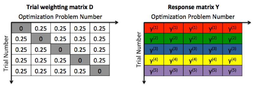
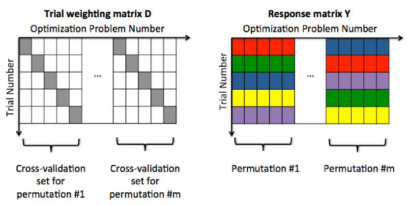
Under cross-validation and bootstrapping, the variability in arises through problem-specific , while permutation testing utilizes distinct . Thus, we may characterize the entire set of problems arising from any combination of cross-validation, bootstrapping, and permutation testing by matrices and , in which the columns of and contain the trial weighting vector and response vector that correspond to the problem. Example problem structures are illustrated in Figure 1.

3 The FaSTGLZ Algorithm
This section presents the FaSTGLZ algorithm. After introducing the major components of the algorithm in Sections 3.1 and 3.2, we offer a discussion on the algorithm’s memory overhead in Section 3.3, as well as extensions of the algorithm to other loss functions and regularizers, including the group lasso in Section 3.4.
3.1 Simultaneous Newton Solver
We first consider simultaneously solving (8) without the sparsity constraint, by setting . This greatly simplifies the problem by removing the non-differentiable portion of the objective. It also allows us to highlight our simultaneous Newton solver, which is a major component of the complete FaSTGLZ algorithm, and is the main machinery through which the shared structure across problems is leveraged for computational efficiency.
With , our goal reduces to minimizing the objectives :
| (9) |
This amounts to fitting a GLZ with a ridge penalty. This is commonly optimized by iteratively re-weighted least squares (IRLS), which sequentially minimizes a quadratic approximation to (9). Specifically, is approximated by a quadratic function around an estimate :
| (10) |
| (11) | |||||
| (12) |
where and are, respectively, the gradient and Hessian of evaluated at , is the residual error vector and is the Hadamard product. Also, is a diagonal matrix of non-negative values, whose diagonal entry is given by .
Since the Hessian is positive semi-definite, we may solve for the minimum of the quadratic approximation to by setting its gradient to zero. This results in the following system of linear equations:
| (13) |
where . Inverting this linear system, either directly or by an iterative method, would typically be prohibitive since the number of features is assumed to be large and is not a sparse matrix.
At this point, we take advantage of the shared structure in two key ways in order to simultaneously solve (13) across all problems very efficiently. First, analogous to the representer theorem, as described in Kimeldorf and Wahba (1970); Schölkopf et al. (2001), we note that the solution in (13) must lie in the range (column space) of the data matrix for all . This allows us to transform the linear system above into a much lower-dimensional space. Specifically, given a QR-factorization for the data matrix, , with having orthonormal columns and , the solution may be expressed as , where satisfies:
| (14) | |||||
| (15) |
Thus, we have converted the original linear system of equations into a system of equations by projecting into a common low-dimensional space spanned by the columns of . In scenarios, this results in a significant reduction.
The second way that we exploit the shared structure allows us to solve (14) for all problems with only a single matrix inversion and in one linear algebraic expression. Before deriving the method, we first briefly summarize the main ideas. Since the structural form of is highly similar across problems, we first approximate the solution to (14) by inverting a template matrix that is representative of all the . To obtain the exact solution for each , we then employ an iterative algorithm that corrects the errors incurred by approximating each by the template . Since the variability between and arises through the matrix in (15), it cannot be modeled as a low-rank perturbation, for which numerous correction methods exist (see Golub and Loan, 1996). Instead, we base our iterative correction algorithm on the theory of stationary iterative methods for solving linear systems of equations (Young, 1971).
Stationary iterative methods provide a simple and efficient framework for solving linear systems without resorting to inverting . Instead, is decomposed into an additive splitting of two matrices , where the inverse of is known or easily computable, and is the residual. The linear system is then solved by computing a sequence of iterates:
| (16) |
Convergence to the solution is guaranteed as long as the spectral radius of is less than one (Young, 1971). Intuitively, this provision requires that the template sufficiently resembles .
Rather than using this technique to invert a single matrix, we will apply it to invert all , . To do so, we define a common template matrix whose inverse we will compute, where is a diagonal matrix of non-negative values that we will specify shortly. We can then express each in terms of the template plus a residual:
| (17) |
Using (16), this splitting implies the following iteration for solving (14):
| (18) |
We prove in the supplementary material that taking the matrix to be the element-wise maximum guarantees that converges to the true solution of (14) for every . See also Conroy and Sajda (2012).
An added benefit of the iteration in (18) is that the updates across can be pooled into a single linear algebraic expression. This greatly simplifies the code and also minimizes memory access times. Let be matrices whose columns contain, respectively, , and , where extracts the main diagonal entries of a matrix into a vector. Then the updates in (18) can be computed as:
| (19) |
Although computing requires operations, this is only performed once at initialization. Otherwise, the complexity of the iteration above is . Thus, computing Newton’s method in this manner scales with the number of problems like instead of (ignoring terms independent of ). Also note that the number of iterations required for the sequence in (19) to converge depends entirely on how well the template matches the true matrices, and is not a function of .
Minimization then proceeds by iteratively updating the quadratic approximation in (10), each time setting to the previously estimated . Since Newton’s method has local quadratic convergence properties (Dennis and Schnabel, 1987), very few iterations are required in practice.
3.1.1 Example of Broader Utility of Simultaneous Newton Solver
Linear systems of the form in (13) arise in a wide array of situations, particularly in optimization problems that may be solved by iteratively re-weighted least squares. Here we highlight the broader utility of our simultaneous Newton solver through an example in time-series regression. Suppose we have a set of time-series , that we would like to linearly regress against a common set of signals, assembled as columns in the matrix :
| (20) |
where is colored Gaussian noise whose temporal auto-correlation structure varies with . Such a model, for example, arises in the univariate General Linear Model in functional magnetic resonance imaging (fMRI) statistical analysis (Woolrich et al., 2001). In this case, the time-series are the measured fMRI signals from a set of brain voxels, and is a design matrix that encodes information about the experimental conditions and confounds. Having the noise auto-covariance depend on allows the model to adapt to the spatially-varying noise properties across the brain.
Given the model above, the best linear unbiased estimator (BLUE) minimizes the negative log-likelihood:
| (21) |
A common assumption in time-series regression is that the noise is generated by an auto-regressive process, in which case there exists a Toeplitz matrix such that . In fact, implements the filter that whitens the noise, and may be estimated by analyzing the covariance of the initial residuals , with minimizing (21) when . Given an estimate for , our original problem (21) reduces to:
| (22) | |||||
| (23) |
This process is repeated for each time-series regression problem .
The solution to (23) can be implemented entirely in the frequency domain and fits naturally into the simultaneous Newton framework proposed above. This approach avoids computing multiple inverse Fourier transforms and matrix inverses. With sufficient zero-padding, the matrices can be made to be circulant, in which case they share a common set of eigenvectors that correspond to the DFT basis. Specifically, can be decomposed as , where is a diagonal matrix that contains the DFT coefficients of the auto-correlation filter, and is the unitary DFT matrix so that produces the DFT coefficients of a signal . Substituting this expression for into (23), we obtain:
| (24) |
where and are the DFT coefficients of the design matrix regressors and response time-series, respectively. Since is a real-valued diagonal matrix, the matrix inversions in (24) may be computed simultaneously as before, with the template matrix taking the form of , and is a diagonal matrix whose entries are the element-wise maxima of .
3.2 FaSTGLZ with sparsity
We now return to the main problem (8), and this time also consider the sparsity-inducing term . In this setting, we base our approach on the optimization framework of alternating direction method of multipliers (ADMM) (Eckstein and Bertsekas, 1992). The reasoning for this decision is two-fold: first, ADMM provides a natural way for us to employ our simultaneous Newton solver that exploits the redundant problem structure; and second, ADMM is flexible enough to accommodate other regularizers, including the group lasso. We explore this extension further in Section 3.4.
For each problem , we divide the objective function in (8) into the sum of two terms: the differentiable portion , and the non-differentiable term . ADMM then formulates an equivalent optimization problem through the addition of an auxiliary variable :
whose augmented Lagrangian may be expressed as:
| (25) |
where are estimates of the Lagrange multipliers and is a penalty parameter. A benefit of minimizing the augmented Lagrangian is that the constraint can be satisfied without taking (Afonso et al., 2010).
Optimization proceeds by alternating between minimizing (25) with respect to while holding fixed, and vice versa. This is equivalent to the symmetric alternating direction augmented Lagrangian method (SADAL) described in Goldfarb et al. (2009). Specifically, the algorithmic steps are:
| (26) | |||||
| (27) | |||||
| (28) | |||||
| (29) |
The resulting subproblems are substantially simpler than the original: optimizing in (26) involves a differentiable objective, while updating in (28) reduces to a soft-thresholding operation.
For our purposes, it is more convenient to re-parameterize the algorithmic steps in terms of a variable , which is related to the Lagrange multiplier estimates . Specifically, given initial values for , we initialize to . Then the ADMM procedure is equivalent to:
| (30) | |||||
| (31) | |||||
| (32) | |||||
| (33) |
where
| (34) |
and . Also, is the soft-thresholding operator. The equivalence between (26)-(29) and (30)-(33) is shown in the supplementary material.
Note that the updates in (31-33) are computable in closed-form and the only remaining challenge is minimizing the smooth function in (30). Minimizing , however, is almost completely analogous to the ridge-penalized GLZ in (9), except for the extra linear term . This allows us to apply our simultaneous Newton’s method solver to (30) with only a slight modification. As before, we sequentially minimize by taking a quadratic approximation to around an initial estimate . Then, given a QR-factorization of the data matrix , we prove in the supplementary material that the minimum to the quadratic approximation to is attained at:
| (35) |
where is the projection onto , and satisfies:
| (36) |
The are then computed simultaneously for all using the techniques outlined in Section 3.1 for solving (14). As before, (36) can be solved for all with only one matrix inversion and in one linear algebraic expression.
3.3 Reducing memory overhead
As formulated thus far, must be stored in full for each , which requires memory elements. Since is often very large, this places a practical constraint on the number of problems that may be solved simultaneously. This memory overhead can be significantly reduced by employing the recently proposed screening rules for -regularized problems to estimate the active set of each problem (Tibshirani et al., 2012). These tests are based on correlations between the features and the response variable, and can thus be evaluated very efficiently.
Given an estimate of the active set for each , we soft-threshold in (32) only to the active set . Thus, is a sparse vector. Additionally, we show here that the algorithmic steps in (30)-(33) may be computed by only storing , , and the sparse set of entries of restricted to . This is an important point because even though the support of is always confined to the current estimate of the active set, and are not necessarily sparse vectors over all iterations. So our memory overhead has been reduced to , where . Since , this is more scalable for moderate sparsity levels.
To illustrate, assume we are given initial conditions for , and the elements of belonging to . Upon minimizing (30) by solving for from the linear system in (36), we must update both and through (31). Using the expression for in (35), this can be computed as:
| (37) | |||||
| (38) | |||||
| (39) |
Upon updating by soft-thresholding the entries of belonging to , the second update of in (33) is straightforward:
| (40) | |||||
| (41) |
The above updates are computed using only , and . Also, since the soft-thresholding step only requires the elements of at , and the updates for each element of in (38) and (40) do not depend on any other elements of , we only store the elements of belonging to . Aside from the reduced memory load, this insight also improves the computational complexity of these updates. Specifically, the matrix multiplication by in (38) must only be computed amongst the rows of that belong to . This reduces the number of multiplications to from . The other multiplication by in (41) also requires only multiplications.
We can make the memory constraint explicit by estimating the maximum amount of memory required as a function of and , where is the maximum allowable number of features to include in each model. Since sparsity is desirable, is usually capped at a small fraction of the total number of features. The amount of memory, in units of bytes, is given by:
| Memory | ||||
Assuming that , the amount of memory required grows with the number of problems at a rate roughly proportional to . To better contextualize this, consider a machine learning dataset with features and trials. Capping the number of allowable features included in the model at , the amount of memory required in megabytes as a function of is MB. Thus, more than problems can be solved simultaneously with GB of RAM.
Table 2 provides a description of the main variables used by the algorithm.
| Variable | Dimension | Description |
|---|---|---|
| Scalar | The feature space dimension (number of voxels) | |
| Scalar | The number of trials | |
| Scalar | The total number of problems to be solved for | |
| The data matrix (features x trials) | ||
| Orthonormal basis for the range of | ||
| The trial weighting vector for the problem | ||
| The response vector to predict for the problem | ||
| Discriminative weights for the problem | ||
| Lagrange multipliers for ADMM procedure |
3.4 Extensions of the FaSTGLZ Algorithm
In this section we discuss extensions of our FaSTGLZ algorithm to solving (1) for other loss functions and regularizers. We first discuss regularizers other than just the elastic net, and then move to loss functions other than those derived from GLZ’s.
As mentioned previously, ADMM is a flexible technique that can accommodate regularizers other than just the elastic net. Let be the regularization penalty, where is some possibly non-differentiable penalty function. Employing the ADDM splitting technique as before, we set and obtain the following augmented Lagrangian:
| (42) |
In pursuing the alternating minimization strategy as in (30-33), only the minimization with respect to differs from before. Specifically, we end up with the following update:
| (43) |
where, as before, . This minimization is often called the proximity operator of the function (Boyd et al., 2010). It turns out that the proximity operator has a closed-form solution for many useful and popular regularizers. For example, when as in the elastic net, the update results in a soft-thresholding operation.
The group lasso (Yuan and Lin, 2007; Meier et al., 2008) is another example whose proximity operator may be computed in closed-form. The group lasso is useful when prior information allows one to cluster features into distinct groups. The group lasso penalty then encourages sparsity across groups but not within a group, so that features from a group are either all included or all excluded. This penalty may arise in fMRI, for example, given a parcellation that clusters voxels into pre-defined regions-of-interest (ROI). The group lasso would then encourage sparsity across distinct ROI’s, but all voxels in a given ROI selected by the model would contribute. Given a grouping of the features, with denoting the index set of the features belonging to the group, the group lasso penalty is defined as:
| (44) |
Plugging this penalty into (43) results in the following update for the group of features in (Boyd et al., 2010):
| (45) |
This can be seen as a generalization of univariate soft-thresholding to blocks of coordinates: each group of features is either thresholded to zero or shrunk by a constant factor. The FaSTGLZ implementation available online also handles user-specified group lasso penalties. Moreover, FaSTGLZ may in principle apply to any regularizer whose proximity operator is computable in closed-form by making the appropriate adjustment in the update for . A more extensive discussion of proximity operators and those functions that can be computed in closed-form may be found in Boyd et al. (2010).
The FaSTGLZ algorithm may also be extended to loss functions of the form , provided is convex and twice differentiable with respect to its first argument. In this case, the loss function for the problem would be specified by:
| (46) |
This modification requires a change to the update for (see (30)) by replacing the negative log-likelihood term in (34) with the loss function above. Approximating (46) by a quadratic function around results in the same structural form for the gradient and Hessian in (11) and (12), with and the diagonal of , denoted , being replaced by:
| (47) | |||||
| (48) |
Since is assumed to be convex, the diagonal entries of are non-negative, and Newton’s method will converge to the global minimum. With these changes to and , optimization then follows analogously to (30).
4 Results
The FaSTGLZ algorithm is most applicable to datasets in which the number of features greatly exceeds the number of examples (the problem). This situation arises in many applications, but this section highlights examples in neuroimaging. In this setting, the goal is to identify multi-variate patterns from a subject’s brain scans that can decode various markers of cognitive state related to a task or stimulus condition (Haxby et al., 2001; Norman et al., 2006; Sajda et al., 2009). Before presenting the results of our algorithm, we briefly introduce the two experimental datasets: one in functional MRI (fMRI) and one in electroencephalography (EEG).
4.1 Data Description
In the fMRI experiment, subjects participated in an auditory oddball detection task. On each trial, the subject was presented with a standard tone (a pure Hz pure tone) of the time, or an oddball tone (a broadband “laser gun” sound) the remaining of the time, and the subject was told to respond via button-press when an oddball stimulus was perceived. Throughout the experiment, fMRI data were collected, and details on data preprocessing can be found in (Goldman et al., 2009; Walz et al., 2012). The decoding task is to predict the stimulus category of each trial from the fMRI data. Since there are two categories (oddball/standard), the GLZ is equivalent to logistic regression. For each of subjects, trials were acquired, and features corresponded to the fMRI response from brain voxels, with .
In the EEG experiment, subjects participated in a three-alternative forced choice visual discrimination task. On each trial, the subject was presented with an image of either a face, car, or house for ms, and had to respond with the category of the image by pressing one of three buttons. To modulate the difficulty of the task, the phase coherence of the presented images were corrupted at one of two levels ( or ), which resulted in “easy” and “difficult” trials. A logistic regression GLZ could likewise be used to predict the difficulty (easy or hard) of each trial from the measured EEG data. The feature data are spatio-temporal voltages measured across scalp electrodes and sampled at Hz between stimulus onset and ms post-stimulus. Treating each electrode-timepoint pair as a feature resulted in features ( electrodes time points, plus a bias term). The number of trials was .
4.2 FaSTGLZ Results
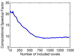
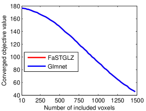
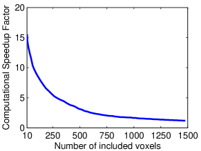
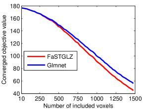
First, we benchmarked the speed of FaSTGLZ in solving a set of problems against solving them sequentially using the popular glmnet algorithm using coordinate descent (Friedman et al., 2010). Following Friedman et al. (2010), we parameterized the regularization parameters in terms of and held fixed, while varied along a regularization path of values. As an example of a significance testing problem, we trained the classifier along this regularization path for permutations, and compared the time required by the two algorithms. Figure 2 plots the computational speedup factor, defined as the ratio of time required by glmnet to the time required by FaSTGLZ, as a function of the average number of voxels included in the model. FaSTGLZ is at a minimum x faster. We verified that the relative difference in the converged objective value between the two algorithms never exceeded , and a plot of the converged objectives is shown in Figure 2. As a further check, we also increased the convergence tolerance on glmnet so that it ran the full regularization path in roughly the same time as FaSTGLZ (FaSTGLZ was still x faster – see Figure 2). In this case, FaSTGLZ produced a converged objective value that was approximately lower than glmnet (see Figure 2).
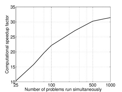
To directly test the efficiency garnered by exploiting the shared structure across problems, we repeated the above analysis, but instead benchmarked FaSTGLZ against itself without simultaneity, i.e., running FaSTGLZ sequentially on each of the problems. We then ran FaSTGLZ numerous times, varying the number of optimization problems that were simultaneously solved on a log scale. Figure 3 plots the computational speedup factor relative to the non-simultaneous FaSTGLZ as a function of . The graph has an initial rapid rise so that with , the speedup is around x, and there is an inflection point at around simultaneous problems (speedup of x), after which point there is a diminishing rate of return in efficiency. Interestingly, the base FaSTGLZ algorithm without simultaneity is about x slower than glmnet. This further emphasizes that the empirical computational improvement relative to glmnet in the previous example is directly a result of exploiting the shared structure across problems.
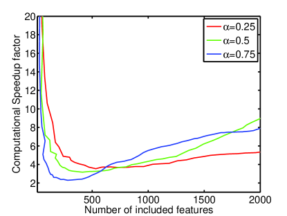
We also benchmarked FaSTGLZ on the EEG example dataset described in Section 4.1. In this instance, we compared the speed of FaSTGLZ in solving a set of problems derived via bootstrapping against solving them sequentially using glmnet. For each problem, the training set was derived by sampling with replacement from the set of trials. The weight assigned to trial for problem was then set to the number of times that trial was sampled in the bootstrap. The regularization parameter was varied along a regularization path of values for each of values of . Figure 4 plots the computational speedup factor of FaSTGLZ relative to glmnet as a function of the number of features included in the model for each value of . Again, the relative difference in converged objective values was observed to never exceed .
5 Conclusion
We presented the fast simultaneous training of generalized linear models (FaSTGLZ) algorithm and demonstrated its significant speedup in computational efficiency when analyzing high-dimensional real-world datasets. FaSTGLZ enables efficiently training families of elastic-net regularized GLZ models that may arise from bootstrapping, cross-validation, and permutation testing. We also provided a discussion on extensions of the algorithm to other regularizers and loss functions, including group lasso. Moreover, by appropriately setting the elastic net regularization parameters, ridge and lasso are also accommodated as special cases.
The FaSTGLZ algorithm is particularly efficient when the number of examples is limited, but the number of features may be very large (the problem). This is often the case in many real-world scenarios, including neuroimaging datasets such as EEG, MRI, and DTI, as well as genetic datasets.
From the algorithmic perspective, there are a number of future research directions. Boyd et al. (2010) showed that ADMM can be coupled with distributed optimization to effectively handle very large-scale datasets (large and ). Connecting this approach with our FaSTGLZ algorithm could potentially be very fruitful. Another potential research direction is in making simultaneous versions of other machine learning algorithms. For example, faster variants of ADMM have been presented recently in Goldfarb et al. (2009); Goldstein et al. (2012). Adapting these algorithms to simultaneous versions could further improve computational efficiency.
Acknowledgments
This work was supported by National Institutes of Health grant R01-MH085092, the National Science Foundation Graduate Research Fellowship Program, and by the Army Research Laboratories under Cooperative Agreement Number W911NF-10-2-0022. The views and conclusions are those of the authors and should not be interpreted as representing the official policies, either expressed or implied, of the Army Research Laboratory or the U.S. Government.
We thank Jordan Muraskin, Robin Goldman, and Eftychios Pnevmatikakis for their fruitful discussions and suggestions. We also thank Glenn Castillo and Stephen Dashnaw for their assistance with EEG-fMRI data acquisition.
Supplementary Material
Proof of convergence of simultaneous Newton’s method iterative solver (see §3.1)
Here we show that by taking the template matrix to be , with the element-wise maximum, then the iterative method:
| (49) |
converges to the true solution of (14) for each .
First note that if (49) does converge for some , then is the solution to (14). To see this, note that upon convergence , and plugging that into (49), we have:
| (50) | |||||
| (51) | |||||
| (52) | |||||
| (53) |
where the second step above used the fact that .
To prove convergence, we must show that the spectral radius of is less than one Young (1971). To simplify notation, let . Since the eigenvalues of correspond to the generalized eigenvalues , we may compute the spectral radius by maximizing the generalized Rayleigh quotient:
| (54) |
Taking assures that and are positive semi-definite matrices for all . As a result, the numerator and denominator of (54) are real, non-negative numbers. As a result, constraining requires that for all vectors :
| (55) | |||||
| (56) | |||||
| (57) |
Thus, (49) converges provided that for all , which is guaranteed since is PSD and .
Equivalence of ADMM Procedures ((26)-(29)) and ((30)-(33)) (see §3.2)
Here we show that the standard ADMM procedure (26)-(29) is equivalent to the modified procedure (30)-(33). First, we expand (26) as:
Proof of (35) (see §3.2)
First, we establish that the solution must lie in . To show this, take any vector . Then taking the inner product of with both sides of (34), we obtain:
| (64) | |||||
| (65) |
The above follows from the fact that and for any , (see equations (11) and (12)). Therefore, , implying that .
At this point, we impose a change of basis by expressing , where the columns of span the orthogonal complement of . This gives us:
| (73) | |||
| (80) |
Thus, and is the solution to:
| (81) |
which is the same as that given in (36). Substituting into our original expansion for : , we obtain:
| (82) | |||||
| (83) |
which completes the proof.
References
- Afonso et al. (2010) M.V. Afonso, J.M. Bioucas-Dias, and M.A.T. Figueiredo. Fast image recovery using variable splitting and constrained optimization. IEEE Transactions on Image Processing, 19(9):2345–2356, 2010.
- Boyd et al. (2010) S. Boyd, N. Parikh, E. Chu, B. Peleato, and J. Eckstein. Distributed optimization and statistical learning via the alternating direction method of multipliers. Foundations and Trends in Machine Learning, pages 1–122, 2010.
- Conroy and Sajda (2012) B. Conroy and P. Sajda. Fast, exact model selection and permutation testing for -regularizaed logistic regression. In N. Lawrence and M. Girolami, editors, Proc. International Conference on Artificial Intelligence and Statistics, JMLR C & WP, pages 246–254, 2012.
- Dennis and Schnabel (1987) J.E. Dennis and R.B. Schnabel. Numerical Methods for Unconstrained Optimization and Nonlinear Equations. Society for Industrial Mathematics, 1987.
- Eckstein and Bertsekas (1992) J. Eckstein and D. Bertsekas. On the douglas-rachford splitting method and the proximal point algorithm for maximal monotone operators. Mathematical Programming, 55(1):293–318, 1992.
- Friedman et al. (2010) J. Friedman, T. Hastie, and R. Tibshirani. Regularization paths for generalized linear models via coordinate descent. J. Stat. Soft., 33(1):1–22, 2010.
- Goldfarb et al. (2009) D. Goldfarb, S. Ma, and K. Scheinberg. Fast alternating linearization methods for minimizing the sum of two convex functions. Technical report, Columbia University, New York, NY, 2009.
- Goldman et al. (2009) R.I. Goldman, C.Y. Wei, M.G. Philiastides, A.D. Gerson, D. Friedman, T.R. Brown, and P. Sajda. Single-trial discrimination for integrating simultaneous EEG and fMRI: Identifying cortical areas contributing to trial-to-trial variability in the auditory oddball task. NeuroImage, 47(1):136–147, 2009.
- Goldstein et al. (2012) T. Goldstein, B. O’Donoghue, and S. Setzer. Fast alternating direction optimization methods. Technical report, UCLA, 2012.
- Golland et al. (2005) P. Golland, F. Liang, S. Mukherjee, and D. Panchenko. Permutation tests for classification. In Proc. COLT: Annual Conference on Learning Theory LNCS, volume 3559, pages 501–515, 2005.
- Golub and Loan (1996) G.H. Golub and C.F. Van Loan. Matrix Computations. Johns Hopkins University Press, 1996.
- Haxby et al. (2001) J.V. Haxby, M. Gobbini, M. Furey, A. Ishai, J. Schouten, and P. Pietrini. Distributed and overlapping representations of faces and objects in ventral temporal cortex. Science, 293(5539):2425–2430, 2001.
- Kimeldorf and Wahba (1970) G.S. Kimeldorf and G. Wahba. A correspondence between bayesian estimation on stochastic processes and smoothing by splines. The Annals of Mathematical Statistics, 2111:416–426, 1970.
- McCullagh and Nelder (1989) P. McCullagh and J.A. Nelder. Generalized Linear Models. Chapman and Hall, 1989.
- Meier et al. (2008) L. Meier, S. van d Geer, and P. Buhlmann. The group lasso for logistic regression. Journal of the Royal Statistical Society, Series B, pages 53–71, 2008.
- Norman et al. (2006) K.A. Norman, S.M. Polyn, G.J. Detre, and J.V. Haxby. Beyond mind-reading: multi-voxel pattern analysis of fMRI data. Trends in Cog. Sci., 10(9):424–430, 2006.
- Sajda et al. (2009) P. Sajda, M.G. Philiastides, and L.C. Parra. Single-trial analysis of neuroimaging data: Inferring neural networks underlying perceptual decision making in the human brain. IEEE Reviews in Biomedical Engineering (invited), 2:97–109, 2009.
- Schölkopf et al. (2001) B. Schölkopf, R. Herbrich, A.J. Smola, and R.C. Williamson. A generalized representer theorem. In Proceedings of the Annual Conference on Computational Learning Theory, pages 416–426, 2001.
- Tibshirani (1996) R. Tibshirani. Regression shrinkage and selection via the lasso. Journal of the Royal Statistical Society, Series B, 58:267–288, 1996.
- Tibshirani et al. (2012) R. Tibshirani, J. Bien, J. Friedman, and T. Hastie. Strong rules for discarding predictors in lasso-type problems. J.R. Statist. Soc. B, 74:245–266, 2012.
- Walz et al. (2012) J.M. Walz, R.I. Goldman, J. Muraskin, T.R. Brown, and P. Sajda. Simultaneous EEG-fMRI reveals a superposition of task-dependent and default-mode networks during a simple target detection task. NeuroImage (submitted), 2012.
- Woolrich et al. (2001) M.W. Woolrich, B.D. Ripley, M. Brady, and S.M. Smith. Temporal autocorrelation in univariate linear modeling of fmri data. NeuroImage, 14:1370–1386, 2001.
- Young (1971) D.M. Young. Iterative solution of large linear systems. Dover Publications, 1971.
- Yuan and Lin (2007) M. Yuan and Y. Lin. Model selection and estimation in regression with grouped variables. Journal of the Royal Statistical Society, Series B, 1:49–67, 2007.
- Zuo and Hastie (2005) H. Zuo and T. Hastie. Regularization and variable selection via the elastic net. J.R. Statist. Soc. B, 67(2):301–320, 2005.