Cosmic ray Spectrum, Composition, and Anisotropy Measured with IceCube

Abstract

Analysis of cosmic ray surface data collected with the IceTop array of Cherenkov detectors at the South Pole provides an accurate measurement of the cosmic ray spectrum and its features in the ”knee” region up to energies of about 1 EeV. IceTop is part of the IceCube Observatory that includes a deep-ice cubic kilometer detector that registers signals of penetrating muons and other particles. Surface and in-ice signals detected in coincidence provide clear insights into the nuclear composition of cosmic rays. IceCube already measured an increase of the average primary mass as a function of energy. We present preliminary results on both IceTop-only and coincident event analyses. Furthermore, we review the recent measurement of the cosmic ray anisotropy with IceCube.

1 IceCube and Cosmic Rays

Acceleration of galactic cosmic particles in the shock waves of nearby supernova remnants is believed to produce the features observed in the energy spectrum of primary particles detected at Earth. The gradual steepening of the cosmic ray flux at a few 10¹⁵ eV, called the knee, and other structures at higher energies are interpreted as the signatures of these sources [1, 2]. The transition from galactic to extragalactic components of cosmic particles is predicted [3] at a few 10¹⁷ eV or 10¹⁸ eV depending on whether the extragalactic component is purely protonic or a mixture of different nuclei. At energies between 10¹⁵ eV to 10¹⁷ eV, all air shower experiments observe an increase in the measured average mass, compatible with an energy dependent change of cosmic ray composition. Above 10¹⁷ eV and up to 10¹⁸ eV, measurements of composition indicate a decrease of the average mass [4].

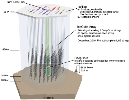
Figure 1: Sketch of the IceCube Observatory. IceCube in its 2006-07 configuration is shown in red and referred to as IT26/IC22 (26 IceTop stations/22 in-ice cables). Other configurations are IT40/IC40 (2007-08) in green, IT59/IC59 (2008-09) in purple, IT73/IC79 (2009-10) in blue, and IT81/IC86 (2010-11 and subsequent seasons) in yellow.

IceCube (Fig. 1) is a multi-purpose astrophysical observatory installed at the South Pole in operation since 2005 [5]. It consists of a surface array of Cherenkov tanks, called IceTop, and a large array of optical modules in the deep ice between 1.45 and 2.45 km below the ice sheet. Data of the surface array allow reconstructing direction and energy of down-going primary cosmic rays in the energy range from about 100 TeV to 1 EeV. The main purpose of the deep detector array is to detect neutrinos, but it also permits the reconstruction of penetrating cosmic ray muons [6]. Since May 2011, IceCube is taking data in its full configuration. The deep detector is an array of 86 cables (“strings”), each instrumented with 60 digital optical modules [7] (DOMs). A DOM contains photomultipliers and readout electronics.

Near the top of each string at an altitude of 2835 m a.s.l. (atmospheric depth of about 680 g/cm²), 81 pairs (“stations”) of cylindrical Cherenkov tanks form IceTop, covering an area of about 1 km² [8]. Each tank contains two standard IceCube DOMs and samples secondary particles (low-energy photons, electrons, and muons) from air showers. At the time of deployment, the top of each tank was at the same level as the surrounding snow. However, snow drifting causes the overburden to increase with time. The snow depth over each tank is physically measured every year and can be indirectly estimated from the muon/electron ratio in calibration curves (Fig. 2).

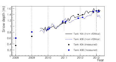
Figure 2: Accumulation of snow over time, for the two tanks of one IceTop station [9]. Direct measurements of snow depth are shown with solid symbols. Indirect measurements using calibration curves (VEMCal data) are shown with lines.

IceTop DOM charges are calibrated using signals from single muons, expressed as an independent unit called “Vertical Equivalent Muon” (VEM) [8].

At the altitude of IceTop, secondary particles are sampled near the shower maximum. This allows precisely measuring the energy spectrum of primary cosmic rays with an energy resolution of about 10% above 10¹⁶ eV (10 PeV). Events seen in coincidence by both IceTop and the deep detector (see Fig. 3) give clear insights into the nuclear composition of cosmic rays for energies that span from PeV to EeV (10¹⁸ eV). The deep detector measures the signal of penetrating muons (more than about 500 GeV at production) from the early stage of shower development. The in-ice DOMs detect the light emitted due to energy loss of high energy muons inside the detector volume. The amount of Cherenkov light generated is proportional to the deposited energy, which is in good approximation a function of the muon multiplicity alone. At a fixed time, the light collected from these muons has traveled a certain distance and the coherent wave front of photons emitted at a given time is used to reconstruct track direction and energy loss profile. Penetrating muons are more abundant in iron showers than in proton showers since shower development starts higher in the atmosphere. The in-ice signal of iron showers is therefore larger for a given energy and zenith angle.

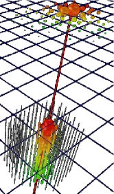
Figure 3: Cosmic ray coincident event recorded by IceCube in 2010. Triggered DOMs are indicated with colored spheres whose volume is proportional to the registered signal. Signal times are indicated with colors from red to green, red being the earliest. This event is reconstructed with an energy of 3$\cdot$10¹⁷ eV and a zenith angle of 11.5^∘. Additional information on surface and in-ice reconstruction is given in Figs. 4 and 8, Sec. 2 and 3.

During the construction phase, IceTop measured the cosmic ray energy spectrum at energies between 1 PeV and 100 PeV when only 26 stations were operational [10]. Using coincident events, the cosmic ray spectrum and average nuclear composition were measured between 1 PeV and 30 PeV [11]. Furthermore, the large statistics and good angular resolution allowed detection of cosmic ray anisotropies in the Southern sky at the per-mille level on angular scales down to a few degrees [12, 13].

This paper emphasizes and highlights the latest results from analyses of cosmic ray events collected with 73 stations of IceTop (IT73) and 79 cables of IceCube (IC79). The latest measurements of energy spectrum and composition cover the energy range from about 1 PeV to 1 EeV and include zenith angles up to about 40^∘. Only events with reconstructed shower cores contained within the IceTop array were considered. In Sec. 2 the primary energy spectrum obtained with events of IT73-only is presented. In Sec. 3 the measurement of composition with coincident events of IC79/IT73 is discussed. In Sec. 4 a recent study of the anisotropy comparing IceTop and deep detector measurements is reviewed. An outlook on the status of the extension of the current analysis to include more inclined events is given in Sec. 5.

2 Cosmic ray Primary Spectrum with IceTop

Using data taken between June 1, 2010 and May 13, 2011 (effective livetime of 327 days), about 37 million events of cosmic rays were reconstructed. These events are a selection of IceTop events with $\cos\theta>$ 0.8 ($\theta<$ 37^∘) and triggering 5 or more stations. For the analysis, only “contained” events were considered. These events had reconstructed cores within an area delimited by the outermost stations.

The surface shower particle density decreases rapidly with the distance from the shower axis. This lateral distribution function (LDF) carries information about the energy of the primary particle. The charge expectation value $S$ in an IceTop tank at distance $r$ from the shower axis is described by a “double logarithmic parabola” [8]

$$S(r)=S_{125}\cdot\left(\frac{r}{125}\right)^{-\beta-\kappa\log_{10}(r/125)},$$ (1)

where $S_{125}$ is the charge in VEM at 125 m (Fig. 4).

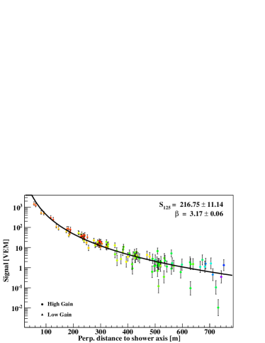
Figure 4: Lateral distribution of tank signals in VEM for the event in Fig. 3 fitted to the function in Eq. 1. Below 100 m, saturation starts becoming evident with signals around 1500 VEM, but it does not impact significantly $S_{125}$. DOMs are completely saturated at about 3000 VEM.

This description is empirical and derived from simulation. In log-log format, $\beta$ represents the slope of $\log_{10}S(r)$ at 125 m and $\kappa$ represents its curvature. Assuming a fixed value of $\kappa=$ 0.303 was verified not to impair reconstruction quality of simulated events. Signals measured between about 30 m and 300 m from the shower axis are well described by Eq. 1 for primary zenith angles in the range 0^∘–40^∘. For larger angles, the LDF needs to include a description of the muon component as a function of the distance from the shower core (see Sec. 5) The reference distance of 125 m makes $S_{125}$ approximately independent of the primary type and minimizes the correlation between $S_{125}$ and $\beta$. Events with $\log_{10}(S_{125})\leq$ 0 are currently not used in any analysis since they are affected by fluctuations introduced when correcting the signals to account for the snow coverage. Correct treatment of events below this threshold is under investigation.

Snow coverage affects the measurement of $S_{125}$. Expected tank signals are therefore corrected by using the following equation [9]

$$S_{corr}(r)=S(r)\cdot exp(-X/\lambda_{s}),$$ (2)

where $X=d_{snow}/\cos\theta$ is the slant depth that particles must traverse to the tank at a depth $d_{snow}$, and $\lambda_{s}$ is an attenuation length fixed to 2.1 m. A maximum likelihood method is used to derive $S_{125}$ and zenith angle from integrated charges and leading edge times of waveforms [8]. This likelihood includes an additional term describing signal saturation (see Fig. 4).

The energy of the primary cosmic ray is estimated from the relationship between $S_{125}$ and the true primary energy, $E_{true}$, derived from simulations. The 2-dimensional histogram of $\log_{10}S_{125}$ $vs$ $\log_{10}E_{true}$ for simulated proton showers with $\cos\theta>0.95$ is shown in Fig. 5.

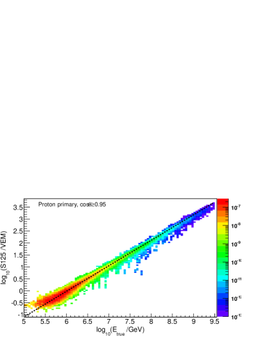
Figure 5: $\log_{10}S_{125}$ $vs$ $\log_{10}E_{true}$ for simulated events of proton primaries with $\cos\theta>$0.95 and triggering 5 or more stations. The histogram is weighted with $E^{-2.7}$. For a measured $\log_{10}S_{125}$, the dashed line can be used to identify the most likely true primary energy (see text for details).

The relationship between $\log_{10}S_{125}$ and $\log_{10}E_{true}$ depends on the mass of the primary particle and the zenith angle of its arrival direction. For any measured $\log_{10}S_{125}$ within a bin of size $\Delta\log_{10}S_{125}=$ 0.05, the reconstructed energy ($\log_{10}E$) is the mean of the fitted distribution of the corresponding $\log_{10}E_{true}$ values. The impact of a change of about 1 unit in the spectral index (from -2.6 to -3.5) used to weight the 2-dimensional histogram of $\log_{10}S_{125}$ $vs$ $\log_{10}E_{true}$ is negligible and corresponds to a shift of the mean of $\log_{10}E_{true}$ distributions which is smaller than $\Delta\log_{10}E_{true}=$ 0.05. Consequently, the relationship between primary and reconstructed energy is not spectrum-dependent.

Because of mass-dependent energy reconstruction biases, to derive the all-particle energy spectrum, a specific assumption for the primary composition of the detected cosmic ray events has to be made. Assuming an isotropic flux of cosmic rays, one expects that the energy spectrum is invariant with respect to the zenith angle. Energy reconstruction biases do depend on the zenith angle, therefore an incorrect composition assumption leads to a misalignment between measurements at different angles. In this paper and in Ref. [14] the final result is given using the composition assumption corresponding to the $H4a$ model described in Ref. [15]. The choice of this specific model is justified by a reasonable agreement of the measured angular spectra in different energy bands (Fig. 6).

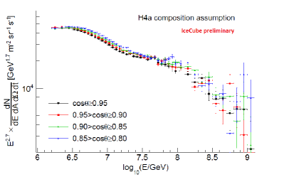
Figure 6: IT73 cosmic ray spectrum in four different zenith angle bins assuming a primary composition based on the H4a (see text for detail).

To unfold the final spectrum and determine its shape, an iterative procedure was used. At each step the spectrum is evaluated based on the effective area and the relationship $\log_{10}S_{125}$ $vs$ $\log_{10}E_{true}$ from the previous step. The fractional contributions of the elemental groups of the H4a model was kept throughout the procedure. Starting with a featureless power law spectrum, the final spectrum was obtained after two iterations.

In Fig. 7 the measured all-particle energy spectrum is shown with its systematic and statistical uncertainties.

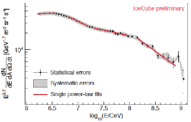
Figure 7: Cosmic ray energy spectrum assuming a composition corresponding to the H4a model. Systematic and statistical uncertainties are shown along with spectral fits in four different energy ranges (see Tabs. 1,2 ).

The all-particle energy spectrum does not follow a single power law above the knee measured at about 4.4 PeV. The spectrum was fitted by a power law function proportional to $E^{-\gamma+1}$ in four different energy ranges. The selected ranges did not include data points where the transition between two power laws was observed.

The spectral index $\gamma$ for the four energy ranges is listed in Tab. 1.

Table 1: Spectral indices with statistical and systematic uncertainties in the four energy ranges of $\log_{10}\left(E/GeV\right)$ shown in Fig. 7.

Energy range	$\gamma\pm$stat.$\pm$sys.	$\chi^{2}/ndf$
6.20–6.55	2.648$\pm$0.002$\pm$0.06	206/2
6.80–7.20	3.138$\pm$0.006$\pm$0.03	14/6
7.30–8.00	2.903$\pm$0.010$\pm$0.03	19/12
8.15–8.90	3.374$\pm$0.069$\pm$0.08	8/6

Above about 18 PeV the spectrum hardens. A sharp drop is observed beyond 130 PeV. The four major systematic uncertainties at two measured energies are summarized in Tab. 2, with the composition assumption being the largest. Two hadronic interaction models were used in simulations: SYBILL2.1 [16] and QGSJETII [17].

Table 2: Systematic uncertainties of the measured flux at two energies. The flux assumes a composition corresponding to the H4a model. The systematic uncertainties include VEM calibration, snow correction, interaction model, and composition assumption.

Energy	Flux Sys.				Total
	VEM	Snow	Inter.	Comp.
3 PeV	+4.0% -4.2%	+4.6% -3.6%	-4.4%	$\pm$7.0%	+9.3% -9.9%
30 PeV	+5.3% -5.3%	+6.3% -4.9%	-2.0%	$\pm$7.0%	+11.0% -10.0

For the same primary energy QGSJETII produced larger $S_{125}$ signals compared to SYBILL 2.1. To estimate the systematics due to composition, the differences between the final and most vertical spectra and the final and most inclined spectra in the primary energy range between $\log_{10}(E/GeV)=$ 6.2 and $\log_{10}(E/GeV)=$ 7.5 were used. This energy range has negligible statistical fluctuations. The total uncertainty on the primary flux is about 10% in all energy ranges.

3 Nuclear Composition of Cosmic Rays with IceCube

Cosmic rays interacting in the atmosphere produce muons. If these muons have enough energy to reach the array of in-ice DOMs of IceCube, they can be used to probe earlier stages of the shower development. For example, depending on the type of the primary particle, proton or iron, an event of 5$\cdot$10¹⁵ eV is expected to produce 30 to 80 muons with sufficient energy to reach a depth of 1500 m. The energy deposited in the deep detector consequently varies from 5$\cdot$10¹² eV to 15$\cdot$10¹² eV. The composition-dependence of the muon multiplicity is the main detection principle used for coincident event analyses. For TeV muons, IceCube mostly detects the Cherenkov light emitted by secondary particles produced in radiative loss processes. Individual catastrophic energy losses can be identified as abrupt increases in the collected light.

Nearly vertical ($\theta\lesssim$ 37^∘ or $\cos\theta>$ 0.8) contained air shower events of IC79/IT73 were analyzed to study the mass composition of cosmic rays [18]. The subsample (30%) of the events described in Sec. 2 and contained in both surface and deep detector were reconstructed with their axis crossing both arrays of IceCube. The energy loss profile of a muon bundle as a function of in-ice depth $\left(dE_{\mu}/dX\right)_{bundle}\left(X\right)$ is derived from amplitude and timing of the signals in the deep optical sensors. The reconstruction takes into account absorption and scattering properties of the surrounding ice. An example is shown in Fig. 8.

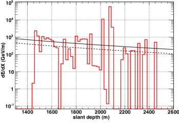
Figure 8: Reconstructed muon bundle energy loss $\left(dE/dX\right)_{bundle}$ as a function of the in-ice depth for the event in Fig. 3. The solid black line is the fitted average energy loss. The dashed line is the average energy loss after removal of stochastic peaks (see text for detail). The highest peak, located at a depth with exceptionally strong dust concentration, and bins with zero energy loss are artifacts of the reconstruction algorithm.

The energy loss at a fixed depth depends mainly on the muon multiplicity, thus being a composition sensitive observable.

Charged mesons, mainly kaons and pions, either decay into high-energy muons or re-interact, depending on the local air density. A correction procedure is therefore applied to account for the strong seasonal variations of the Antarctic atmosphere [19].

The energy loss of a single muon is given by

$$\frac{dE_{\mu}}{dX}=-b\left(E_{\mu,surf.}+\frac{a}{b}\right)\cdot e^{-bX},$$ (3)

where $a=$ 0.260 GeV/m is the continuous energy loss constant and $b=$ 3.57$\cdot$10^-4 m^-1 the proportional energy loss constant. The profile of a bundle produced by a shower of a primary particle is described with the following equation [20]

$$\left(\frac{dE_{\mu}}{dX}\right)_{bundle}\left(X\right)=\int_{E_{\mu,min}}^{E_{\mu,max}}\frac{dN_{\mu}}{dE_{\mu}}\frac{dE_{\mu}}{dX}dE_{\mu,surf.},$$ (4)

where $dN_{\mu}/dE$ is the energy distribution of the muons in the bundle, $E_{\mu,min}=\frac{a}{b}\left(e^{bX}-1\right)$ the minimum energy a muon needs at the surface to reach the depth $X$, and $E_{\mu,max}\propto E/A$ the maximum energy a muon can obtain from this shower at the surface. Here, $E$ represents the primary energy and $A$ its atomic mass. The muon multiplicity is given by the formula [21]

$$\frac{dN_{\mu}}{dE_{\mu}}=\gamma_{\mu}\kappa(A)\left(\frac{E}{A}\right)^{\gamma_{\mu}-1}E_{\mu}^{-\gamma_{\mu}-1},$$ (5)

where $\gamma_{\mu}=1.757$ is the muon integral spectral index and $\kappa$ a normalization factor that depends on the shower properties. By integrating Eq. 4, an average muon bundle energy loss is obtained

$$\left(\frac{dE_{\mu}}{dX}\right)_{bundle}\left(X\right)=\kappa\cdot\left(\frac{A}{\cos\theta}\right)\cdot e^{-bX}\cdot\gamma_{\mu}\cdot\left(\frac{E}{A}\right)^{\gamma_{\mu}-1}\cdot$$

$$\cdot\left[-\left(\frac{E}{A}\right)^{-\gamma_{\mu}}\cdot\left(\frac{a}{\gamma_{\mu}}-\frac{b}{1-\gamma_{\mu}}\cdot\frac{E}{A}\right)+E_{min}^{-\gamma_{\mu}}\cdot\left(\frac{a}{\gamma_{\mu}}-\frac{b}{1-\gamma_{\mu}}\cdot E_{min}\right)\right].$$ (6)

The reconstructed profile is fitted to this integrated energy loss profile.

A multilayer perceptron neural network (NN) was trained with Monte Carlo simulations of 4 primaries (proton, helium, oxygen, and iron) to solve the non-linear mapping of primary energy, primary mass, and reconstructed variables. The masses were chosen due to their equal distance on a logarithmic scale. The previous analysis of coincident events showed that Si and Fe yield similar outputs [11]. Measurements of the electromagnetic component of the air showers at the surface ($S_{125}$) and the muon component in the ice ($\log_{10}\left(dE/dX\right)_{bundle}$) are the main ingredients used to train the network how to find the best fit to the primary energy and mass. More detail on the analysis can be found in Ref. [18]. Intrinsic shower fluctuations and the relatively large overlap between different primary types in the input variables cause a considerable spread of the NN mass output for a given reconstructed energy bin. An un-binned likelihood fit is used to create template histograms for each simulated mass group and reconstructed energy (Fig. 9).

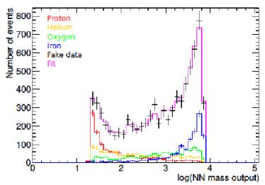
Figure 9: Template histograms for four mass groups in the reconstructed energy bin $\log_{10}E=\left[7.6,7.7\right]$ for a surrogate dataset created from simulations.

Data were passed through the trained NN to obtain a composition-independent energy estimate. The resulting spectrum can be compared to that derived from IceTop-only data (Fig. 10).

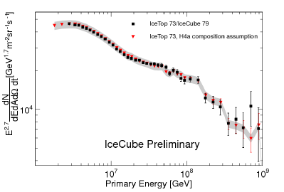
Figure 10: Differential energy spectrum of IC79/IT73 events multiplied by $E^{2.7}$ compared with the IT73-only measurement shown in Fig. 7. A systematic error band of $\pm 7\%$ due to the composition uncertainty is added to the IT73 spectrum.

The coincident event analysis is independent of composition assumptions and the good agreement with the energy spectrum obtained in Sec. 2 demonstrates that selecting the H4a model was a reasonable choice.

For a given reconstructed energy bin, the fractions of each individual mass group (p_H, p_He, p_O, p_Fe) and their uncertainties are known from the template histogram for that bin.

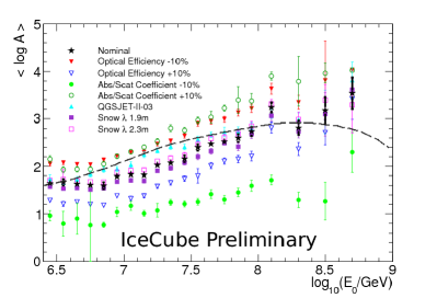
Figure 11: The $<logA>$ composition spectrum as a function of the primary energy obtained with IC79/IT73 data. Systematics are included, dashed line represents the prediction based on the H4a model. This figure is adapted from Ref. [18].

The average mass in the given energy bin is calculated as follows:

$$<logA>=p_{H}logA_{H}+p_{He}logA_{He}+p_{O}logA_{O}+p_{Fe}logA_{Fe}.$$ (7)

The result is shown in Fig. 11. Above about 300 PeV not enough reconstructed events are available from 1 year of data. This results in a larger uncertainty on the solution of template histograms at these energies.

4 Studies of Anisotropy with IceCube

The anisotropy of cosmic ray arrival directions can be measured in two different ways in IceCube [22]: using TeV muon events collected with the deep detector [12, 13] and using air showers triggering the surface array. The in-ice detector has a lower primary energy threshold than IceTop (20 TeV) and can use events at larger zenith angles (up to 70^∘). This makes it possible for the deep detector to reach a higher sensitivity (about 6.3$\cdot$10¹⁰ events/yr, anisotropy level $\delta>$ 10^-5) and scan small scale structures. In Fig. 12 the sky maps in two energy ranges obtained with data collected from IceCube between May 2009 and May 2010 are shown.

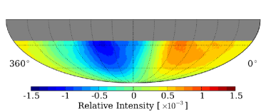
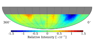
Figure 12: Relative intensity sky maps obtained with IC79. The data sets have median primary energies of 20 TeV (upper) and 400 TeV (lower). The angular binning or smoothing angle is 20^∘. The “deepest” deficits in the lower map is measured with a significance of 6.3$\sigma$.

The main advantage of IceTop is a better energy resolution (20% at $>$300 TeV). Fig. 13 shows the sky maps in two energy ranges obtained with IceTop data collected between May 2009 and May 2011 [23].

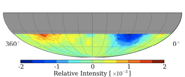
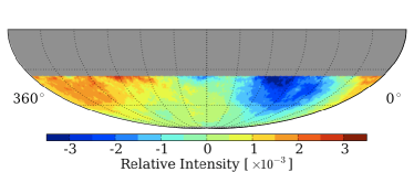
Figure 13: Relative intensity sky maps obtained with IT73 data. The IceTop datasets have a median primary energy of 400 TeV (upper) and 2 PeV (lower). The angular binning or smoothing angle is 20^∘. For the low energy sky map, 2.9$\cdot$10⁸ events and for the high energy sky map, 0.7$\cdot$10⁸ events were used. The “deepest” deficits in both maps are measured with a significance of 7.1$\sigma$.

Only events with zenith angles less than 60^∘ are selected (1.4$\cdot$10⁸ events/yr above 100 TeV, sensitivity to anisotropies $\delta>$ 10^-4). IceTop confirms the large scale anisotropy measured with deep-ice events of IceCube. The result also shows that the global topology of this anisotropy does not change at higher energies. The measurement is inconsistent in both amplitude and phase with the Compton-Getting prediction of an apparent anisotropy caused by the relative motion between the Earth and sources of cosmic rays [24]. A detailed review of possible explanations of the observed topology can be found in Ref. [22].

5 Outlook

In Sec. 2 and 3 results of analysis of nearly vertical events have been presented. In particular, IceTop-only events up to about 40^∘ and coincident IceCube events up to about 30^∘ have been used to scan primary energies above about 1 PeV. Analysis of data collected with a denser sub-array at the center of IceTop will decrease the energy threshold of the detector to about 100 TeV [25].

Another ongoing analysis is trying to identify and reconstruct inclined events up to a zenith angle of 60^∘ [26]. Depending on the primary energy, inclined events above 30^∘ and with their reconstructed shower axis traversing only the in-ice detector volume can leave signals in IceTop tanks. These signals have a larger contribution from the muon component of air showers. Also, inclined events with axis intersecting IceTop but missing the in-ice volume are expected to have a different LDF than the one described here. In fact, the larger amount of matter encountered by secondaries causes their rapid absorption. The use of events contained in only one of the detector components for coincident analyses (Fig. 14) will more than double the current aperture.

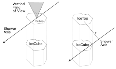
Figure 14: (Left) IceTop-contained showers. The shower axis passes through the IceTop array and misses the in-ice detector. (Right) IceCube-contained showers. The shower axis passes through the in-ice component of IceCube.

For inclined showers, the larger muon contribution (see Fig. 15) needs a modification of the current IceTop LDF, which is optimized for nearly vertical showers whose surface component is mainly dominated by electromagnetic particles.

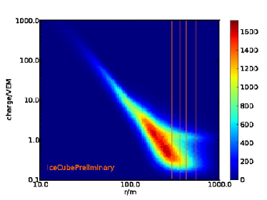
Figure 15: Two-dimensional histogram of the tank total charge as a function of the distance to the shower axis for events with S₁₂₅ between 4 and 5 VEM and zenith angles between 30^∘ and 33^∘. At larger distances from the core (300 m and above) the contribution from single muons becomes apparent as charge clustering around 1 VEM.

The number of muons collected is described by:

$$N_{\mu}(r)=AS_{125}^{\beta}r^{-0.75}\left(1+\frac{r}{320m}\right)^{\gamma}$$ (8)

where $\beta$ and $\gamma$ are parameters that depend on energy and direction of the shower. Knowing the expected number of muons for tanks at large distances from the shower core is the first step towards an energy estimate for inclined showers.

6 Conclusions

Results from analyses performed with data of IT73 and IC79/IT73 have been presented. They can be considered the first comprehensive set of cosmic ray analyses that incorporate detailed studies of the detector performance and systematics conducted during the construction years of IceCube. IceCube is currently taking data in the third year after its completion. Upcoming analyses will yield refined results with smaller systematics and larger statistics, and lead to new understanding about cosmic ray composition and sources. Analysis of coincident events allows the use of the electromagnetic to TeV muon component ratio whose outcome has not been explored before. The goal is to provide a bridge between experiments operating at lower energies around the knee and ultra-high energy detectors at EeV energies. At the moment, the insufficient knowledge of the ice’s optical properties does not allow a better estimate of the absolute average composition.

References

- [1] P. Blasi and E. Amato, JCAP 1201, 010 (2012), arXiv:1105.4521.
- [2] P. Blasi and E. Amato, JCAP 1201, 011 (2012), arXiv:1105.4529.
- [3] R. Aloisio, V. Berezinsky, A. Gazizov, Astropart. Phys. 39-40, 129 (2012).
- [4] K. H. Kampert and M. Unger, Astropart. Phys. 35, 660 (2012).
- [5] A. Achterberg et al. [IceCube Collaboration], Astropart. Phys. 26, 155 (2006).
- [6] I. Taboada for the IceCube Collaboration, these proceedings.
- [7] R. Abbasi et al. [IceCube Collaboration], Nucl. Instrum. Methods A 601, 294 (2009).
- [8] R. Abbasi et al. [IceCube Collaboration], arXiv:1207.6326 (2012).
- [9] IceCube Coll., paper 1106, Proc. of ICRC 2013.
- [10] R. Abbasi et al. [IceCube Collaboration], Astropart. Phys. 44, 40-58 (2013).
- [11] R. Abbasi et al. [IceCube Collaboration], Astropart. Phys. 42, 15-32 (2013).
- [12] R. Abbasi et al. [IceCube Collaboration], Astrophys. J. 718, L194 (2010).
- [13] R. Abbasi et al. [IceCube Collaboration], Astrophys. J. 746, 33 (2012).
- [14] M. G. Aartsen et al. [IceCube Collaboration], arXiv:1307.3795 (2013).
- [15] T. K. Gaisser, Astropart. Phys. 35, 801 (2012).
- [16] E. Ahn et al., Phys. Rev. D 80, 094003 (2009).
- [17] S. Ostapchenko, Nucl. Phys. Proc. Suppl. B 151, 143-146 (2006).
- [18] IceCube Coll., paper 0861, Proc. of ICRC 2013.
- [19] IceCube Coll., paper 0763, Proc. of ICRC 2013.
- [20] T. Feusels et al., in Proc. of ICRC 2009, arXiv:0912.4668.
- [21] J. W. Elbert, in Proc. DUMAND Summer Workshop (ed. A. Roberts), vol. 2, p. 101 (1978).
- [22] P. Desiati for the IceCube Collaboration, these proceedings.
- [23] M. G. Aartsen et al. [IceCube Collaboration], Astrophys. J. 765, 55 (2013).
- [24] A. H. Compton, I. A. Getting, Phys. Rev. 47 817-821 (1935).
- [25] IceCube Coll., paper 0674, Proc. of ICRC 2013.
- [26] IceCube Coll., paper 0973, Proc. of ICRC 2013.