Electroweak Monopole Production at the LHC - a Snowmass White Paper

Abstract

We maintain that the search for the electroweak monopole is a key issue in the advancement of our understanding of the standard model. Unlike the Dirac monopole in electrodynamics, which is optional, the electroweak monopole should exist within the framework of the standard model. The mass of the electroweak monopole is estimated to be 5 to 7 TeV, but could be as large as 15 TeV. Above threshold its production rate at the LHC is expected to be relatively large, $(1/\alpha_{em})^{2}$ times bigger than that of W⁺W^- pairs. The search for the electroweak monopole is one of the prime motivations of the newest LHC experiment, MoEDAL, which is due to start data taking in 2015.

I Introduction

A new particle has recently been discovered at the LHC by the ATLAS and CMS experiments LHC . As more data is analyzed this new particle looks increasingly like the Standard Model Higgs boson. If indeed the Standard Model Higgs boson has been discovered conventional wisdom tells us that this is the final crucial test of the Standard Model. However, we emphasize that there is another fundamental entity that should arise from the framework of the Standard Model - this is the Electroweak (EW), or “Cho-Maison”, magnetic monopole plb97 ; yang . We maintain that the search for the EW monopole is of key importance in advancing our understanding of the Standard Model.

What is the genesis of the Cho-Maison monopole? In electrodynamics the $U(1)$ gauge group need not be non-trivial, so that Maxwell’s theory does not have to have a monopole. Only when the gauge group $U(1)$ becomes non-trivial do we have Dirac’s monopole. In the standard model, however, the gauge group is $SU(2)\times U(1)_{Y}$. The electromagnetic $U(1)_{em}$ comes from the $U(1)$ subgroup of $SU(2)$ and the hypercharge $U(1)_{Y}$. But it is well known that the $U(1)$ subgroup of $SU(2)$ is non-trivial, due to the non-Abelian nature. This automatically makes the $U(1)_{em}$ non-trivial, so that the standard model should have an electroweak monopole plb97 ; yang . So, if the standard model is correct, the Cho-Maison monopole must exist.

It has been asserted that the Weinberg-Salam model has no topological monopole of physical interest vach . The basis for this “non-existence theorem” is that with the spontaneous symmetry breaking the quotient space $SU(2)\times U(1)_{Y}/U(1)_{em}$ allows no non-trivial second homotopy. This claim, however, is unfounded.

Actually the Weinberg-Salam model, with the hypercharge $U(1)$, could be viewed as a gauged $CP^{1}$ model in which the (normalized) Higgs doublet plays the role of the $CP^{1}$ field. So the Weinberg-Salam model does have exactly the same nontrivial second homotopy as the Georgi-Glashow model which allows the ’tHooft-Polyakov monopole plb97 .

The Cho-Maison monopole is the electroweak generalization of the Dirac’s monopole, so that it could be viewed as a hybrid of Dirac and ’tHooft-Polyakov monopoles. But unlike the Dirac’s monopole, it carries the magnetic charge $(4\pi)/e$. This is because in the standard model the $U(1)_{em}$ has the period of $4\pi$, not $2\pi$, as it comes from the $U(1)$ subgroup of $SU(2)$. This makes thesingle magnetic charge of the electroweak monopole twice as large as that of the Dirac Monopole.

II The Electroweak Monopole

Consider the Weinberg-Salam model,

$${\cal L}=-\frac{1}{4}{\vec{F}}_{\mu\nu}^{2}-\frac{1}{4}G_{\mu\nu}^{2}-|D_{\mu}\phi|^{2}-\frac{\lambda}{2}\big{(}|\phi|^{2}-\frac{\mu^{2}}{\lambda}\big{)}^{2},$$

$$D_{\mu}\phi=\big{(}\partial_{\mu}-i\frac{g}{2}\vec{\tau}\cdot{\vec{A}}_{\mu}-i\frac{g^{\prime}}{2}B_{\mu}\big{)}\phi,$$ (1)

where $\phi$ is the Higgs doublet, ${\vec{F}}_{\mu\nu}$ and $G_{\mu\nu}$ are the gauge field strengths of $SU(2)$ and $U(1)_{Y}$ with the potentials ${\vec{A}}_{\mu}$ and $B_{\mu}$. Now choose the static spherically symmetric ansatz

$$\phi=\frac{1}{\sqrt{2}}\rho(r)\xi(\theta,\varphi),~{}~{}~{}\xi=i\left(\begin{array}[]{cc}\sin(\theta/2)\,\,e^{-i\varphi}\\ -\cos(\theta/2)\end{array}\right),$$ (4)

$${\vec{A}}_{\mu}=\frac{1}{g}A(r)\partial_{\mu}t~{}\hat{r}+\frac{1}{g}(f(r)-1)~{}\hat{r}\times\partial_{\mu}\hat{r},$$

$$B_{\mu}=\frac{1}{g^{\prime}}B(r)\partial_{\mu}t-\frac{1}{g^{\prime}}(1-\cos\theta)\partial_{\mu}\varphi.$$ (5)

To proceed notice that we can Abelianize (1) gauge independently using the Abelian decomposition cho . With the gauge independent Abelianization the Lagrangian is written in terms of the physical fields as

$${\cal L}=-\dfrac{1}{2}(\partial_{\mu}\rho)^{2}-\dfrac{\lambda}{8}\big{(}\rho^{2}-\rho_{0}^{2}\big{)}^{2}$$

$$-\dfrac{1}{4}{F_{\mu\nu}^{\rm(em)}}^{2}-\dfrac{1}{4}Z_{\mu\nu}^{2}-\dfrac{g^{2}}{4}\rho^{2}|W_{\mu}|^{2}-\dfrac{g^{2}+g^{\prime 2}}{8}\rho^{2}Z_{\mu}^{2}$$

$$-\dfrac{1}{2}|(D_{\mu}^{\rm(em)}W_{\nu}-D_{\nu}^{\rm(em)}W_{\mu})+ie\dfrac{g}{g^{\prime}}(Z_{\mu}W_{\nu}-Z_{\nu}W_{\mu})|^{2}$$

$$+ieF_{\mu\nu}^{\rm(em)}W_{\mu}^{*}W_{\nu}+ie\dfrac{g}{g^{\prime}}Z_{\mu\nu}W_{\mu}^{*}W_{\nu}$$

$$+\dfrac{g^{2}}{4}(W_{\mu}^{*}W_{\nu}-W_{\nu}^{*}W_{\mu})^{2},$$ (6)

where $\rho$, $W_{\mu}$, $Z_{\mu}$ are the Higgs, $W$, $Z$ bosons, $D_{\mu}^{\rm(em)}=\partial_{\mu}+ieA_{\mu}^{\rm(em)}$, and $e=gg^{\prime}/\sqrt{g^{2}+g^{\prime 2}}$ is the electric charge.

Moreover, the ansatz (5) becomes

$$\rho=\rho(r),~{}~{}~{}W_{\mu}=\dfrac{i}{g}\dfrac{f(r)}{\sqrt{2}}e^{i\varphi}(\partial_{\mu}\theta+i\sin\theta\partial_{\mu}\varphi),$$

$$A_{\mu}^{(em)}=e\Big{(}\dfrac{A(r)}{g^{2}}+\dfrac{B(r)}{g^{\prime 2}}\Big{)}\partial_{\mu}t-\dfrac{1}{e}(1-\cos\theta)\partial_{\mu}\varphi,$$

$$Z_{\mu}=\dfrac{e}{gg^{\prime}}\big{(}A(r)-B(r)\big{)}\partial_{\mu}t.$$ (7)

With this we have the following equations of motion

$$\ddot{\rho}+\frac{2}{r}\dot{\rho}-\frac{f^{2}}{2r^{2}}\rho=-\frac{1}{4}(A-B)^{2}\rho+\frac{\lambda}{2}\big{(}\rho^{2}-\frac{2\mu^{2}}{\lambda}\big{)}\rho,$$

$$\ddot{f}-\frac{f^{2}-1}{r^{2}}f=\big{(}\frac{g^{2}}{4}\rho^{2}-A^{2}\big{)}f,$$

$$\ddot{A}+\frac{2}{r}\dot{A}-\frac{2f^{2}}{r^{2}}A=\frac{g^{2}}{4}\rho^{2}(A-B),$$

$$\ddot{B}+\frac{2}{r}\dot{B}=-\frac{g^{\prime 2}}{4}\rho^{2}(A-B).$$ (8)

Obviously this has a trivial solution

$$\rho=\rho_{0}=\sqrt{2\mu^{2}/\lambda},~{}~{}~{}f=0,~{}~{}~{}A=B=0,$$ (9)

which describes the point monopole in Weinberg-Salam model

$$A_{\mu}^{\rm(em)}=-\frac{1}{e}(1-\cos\theta)\partial_{\mu}\varphi.$$ (10)

This monopole has two remarkable features. First, this is the electroweak generalization of the Dirac’s monopole, but not the Dirac’s monopole. It has the electric charge $4\pi/e$, not $2\pi/e$ plb97 . Second, this monople naturally admits a non-trivial dressing of weak bosons. With the non-trivial dressing, the monopole becomes the Cho-Maison dyon.

Indeed with the boundary condition

$$\rho(0)=0,~{}~{}f(0)=1,~{}~{}A(0)=0,~{}~{}B(0)=b_{0},$$

$$\rho(\infty)=\rho_{0},~{}f(\infty)=0,~{}A(\infty)=B(\infty)=A_{0},$$ (11)

we can show that the equation (8) admits a family of solutions labeled by the real parameter $A_{0}$ lying in the range plb97 ; yang

$$0\leq A_{0}<{\rm min}~{}\Big{(}e\rho_{0},~{}\frac{g}{2}\rho_{0}\Big{)}.$$ (12)

From this we have the electroweak dyon shown in Fig. 1, which becomes the Cho-Maison monopole when $A=B=0$. Since $A_{\mu}^{(em)}$ has the point monopole, the solution can be viewed as a singular monopole dressed by $W$ and $Z$ bosons. This confirms that it can be viewed as a hybrid of the Dirac monopole and the ’tHooft-Polyakov monopole (or Julia-Zee dyon in general).

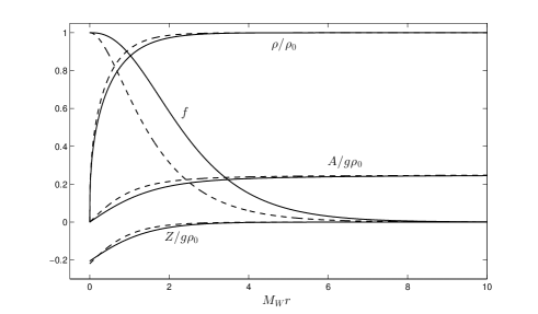
Figure 1: The finite energy electroweak dyon solution. The solid line represents the finite energy dyon and dotted line represents the Cho-Maison dyon, where $Z=A-B$ and we have chosen $f(0)=1$ and $A(\infty)=M_{W}/2$.

To find the monopole experimentally it is important to estimate its mass. At the classical level it carries an infinite energy because of the point singularity at the center, but from the physical point of view it must have a finite energy. To estimate the mass let

$$K_{A}=\dfrac{1}{4}\displaystyle{\int}\vec{F}_{ij}^{2}d^{3}x,~{}~{}~{}K_{B}=\dfrac{1}{4}\displaystyle{\int}B_{ij}^{2}d^{3}x$$

$$K_{\phi}=\displaystyle{\int}|{\cal D}_{i}\phi|^{2}d^{3}x,~{}V_{\phi}=\dfrac{\lambda}{2}\displaystyle{\int}\big{(}|\phi|^{2}-\dfrac{\mu^{2}}{\lambda}\big{)}^{2}d^{3}x,$$ (13)

and divide the energy to infinite and finite parts

$$E=E_{0}+E_{1},$$

$$E_{0}=K_{B},~{}~{}~{}~{}E_{1}=K_{A}+K_{\phi}+V_{\phi}.$$ (14)

With $A=B=0$ we have

$$K_{A}=\dfrac{4\pi}{g^{2}}\displaystyle{\int}_{0}^{\infty}\big{(}\dot{f}^{2}+\dfrac{(f^{2}-1)^{2}}{2r^{2}}\big{)}dr,$$

$$K_{B}=\dfrac{2\pi}{g^{\prime 2}}\displaystyle{\int}_{0}^{\infty}\dfrac{1}{r^{2}}dr,~{}~{}~{}K_{\phi}=2\pi\displaystyle{\int}_{0}^{\infty}(r\dot{\rho})^{2}dr,$$

$$V_{\phi}=\dfrac{\pi}{2}\displaystyle{\int}_{0}^{\infty}\lambda r^{2}\big{(}\rho^{2}-\rho_{0}^{2}\big{)}^{2}dr.$$ (15)

Clearly $K_{B}$ makes the monopole energy infinite. So we have to regularize it to make the monopole energy finite.

Suppose an ultra-violet regularization coming from quantum correction makes $B_{K}$ finite. Now, under the scale transformation

$$\vec{x}\rightarrow\lambda\vec{x},$$ (16)

we have

$$K_{A}\rightarrow\lambda K_{A},~{}~{}~{}K_{B}\rightarrow\lambda K_{B},$$

$$K_{\phi}\rightarrow\lambda^{-1}K_{\phi},~{}~{}~{}V_{\phi}\rightarrow\lambda^{-3}V_{\phi}.$$ (17)

So we have the following energy minimization condition for the stable monopole

$$K_{A}+K_{B}=K_{\phi}+3V_{\phi}.$$ (18)

From this we can infer the value of $K_{B}$. For the Cho-Maison monopole we have (with $M_{W}\simeq 80.4~{}{\rm GeV}$, $M_{H}\simeq 125~{}{\rm GeV}$, and $\sin^{2}\theta_{\rm w}=0.2312$)

$$K_{A}\simeq 0.1852\times\dfrac{4\pi}{e^{2}}{M_{W}},~{}~{}~{}~{}K_{\phi}\simeq 0.1577\times\dfrac{4\pi}{e^{2}}{M_{W}},$$

$$V_{\phi}\simeq 0.0011\times\dfrac{4\pi}{e^{2}}{M_{W}}.$$ (19)

This, with (18), tells that

$$K_{B}\simeq 0.0058\times\dfrac{4\pi}{e^{2}}M_{W},$$

$$E\simeq 0.3498\times\dfrac{4\pi}{e^{2}}M_{W}\simeq 3.85~{}{\rm TeV}.$$ (20)

This strongly implies that the electroweak monopole of mass around 4 TeV could be possible cho .

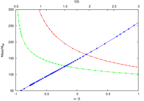
Figure 2: The energy dependence of the electroweak monopole on $\alpha$, $\beta$, or $f(0)$. The red and green curves represents the $\alpha$ and $\beta$ dependence, and the blue curve represents the $f(0)$ dependence.

To backup the above argument, suppose the quantum correction induces the following modification of (6)

$$\delta{\cal L}=ie\alpha F_{\mu\nu}^{\rm(em)}W_{\mu}^{*}W_{\nu}+\beta\frac{g^{2}}{4}(W_{\mu}^{*}W_{\nu}-W_{\nu}^{*}W_{\mu})^{2},$$ (21)

where $\alpha$ and $\beta$ are the quantum correction of the coupling constants. With this we can make the monopole energy finite with

$$f^{2}(0)=\frac{1+\alpha}{1+\beta},~{}~{}~{}~{}~{}\frac{(1+\alpha)^{2}}{1+\beta}=\frac{g^{2}}{e^{2}}.$$ (22)

So only one of the three parameters $\alpha$, $\beta$, $f(0)$, becomes arbitrary. Now, with $f(0)=1$, we have the finite energy monopole with energy $E\simeq 6.72~{}{\rm TeV}$. This is shown in Fig. 1. In general the energy of the monopole depends on the parameter $f(0)$, $\alpha$, or $\beta$, and this dependence is shown in Fig. 2.

This strongly supports our prediction of the monopole mass based on the scaling argument. Moreover, this confirms that a minor quantum correction could regularize the Cho-Maison monopole and make the energy finite cho .

Moreover, in the absence of the $Z$-boson (6) reduces to the Georgi-Glashow Lagrangian when the coupling constant of the quartic self interaction and the mass of the $W$-boson change to $e^{2}/g^{2}$ and $(e^{2}/g^{2})\rho_{0}$. In this case (8) reduces to the following Bogomol’nyi-Prasad-Sommerfield equation in the limit $\lambda=0$ prasad

$$\dot{\rho}\pm\dfrac{1}{er^{2}}\big{(}\dfrac{e^{2}}{g^{2}}f^{2}-1\big{)}=0,$$

$$\dot{f}\pm e\rho f=0.$$ (23)

This has the analytic monopole solution

$$\rho=\rho_{0}\coth(e\rho_{0}r)-\frac{1}{er},$$

$$f=\frac{g\rho_{0}r}{\sinh(e\rho_{0}r)},$$ (24)

whose energy is given by the Bogomol’nyi bound

$$E=\frac{8\pi}{e^{2}}\sin\theta_{\rm w~{}}M_{W}\simeq 5.08~{}{\rm TeV}.$$ (25)

The Cho-Maison monopole, the regularized monopole, and the analytic monopole are shown in Fig. 3. From this we can confidently say that the mass of the electroweak monopole could be around 4 to 7 TeV.

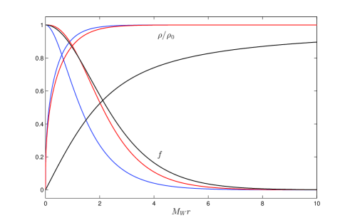
Figure 3: The electroweak monopoles. The blue, red, and black curves represent the Cho-Maison monopole, the regularlized monopole, and the analytic monopole, respectively.

Independent of the details there is a simple argument which can justify the above estimate. Roughly speaking, the mass of the electroweak monopole should come from the same mechanism which generates the mass of the weak bosons, except that the coupling is given by the monopole charge. This means that the monopole mass should be of the order of $M_{W}/\alpha_{em}\simeq$ 10.96 TeV, where $\alpha_{em}$ is the electromagnetic fine structure constant. This supports the above mass estimate cho .

This tells that only LHC could produce the Cho-Maison monopole. If so, one might wonder what is the monopole-antimonopole pair production rate at LHC. Intuitively the production rate must be similar to the WW production, except that the coupling is $4\pi/e$. So above the threshold energy, the production rate can be about $1/\alpha_{em}$ times bigger than that of the WW production rate.

III The MoEDAL Experiment

The MoEDAL experiment MoEDAL is the 7th and latest LHC experiment to be approved. The prime purpose of the MoEDAL experiment is to search for the avatars of new physics that manifest themselves as very highly ionizing particles, such as the Cho-Maison monopole.

The MoEDAL experiment will be deployed at Point 8 on the LHC ring in the VELO-LHCb cavern. It is due to start data taking in 2015, after the long LHC shutdown, when the LHC with be operating at a centre-of-mass energy near to 14 TeV. A simplified depiction of the MoEDAL detector is shown in Fig. 4.

The mean rate of energy loss per unit length $dE/dx$ of a particle carrying an electric charge $q_{e}=ze$ traveling with velocity $\beta=v/c$ in a given material is modelled by the Bethe-Bloch formula bethe :

$$-\frac{dE}{dx}=K\frac{Z}{A}\frac{q_{e}^{2}}{\beta^{2}}\left[ln\frac{2m_{e}c^{2}\beta^{2}\gamma^{2}}{I}-\beta^{2}\right]$$ (26)

where $Z,A$ and $I$ are the atomic number, atomic mass and mean excitation energy of the medium, $K=$ 0.307 MeV g^-1 cm², $m_{e}$ is the electron mass and $\gamma=1/\sqrt{1-\beta^{2}}$. Higher-order terms are neglected.

For a magnetic monopole carrying a magnetic charge $q_{m}=(ng)ec$, where g is the Dirac charge and $n=1,2,3....$, the velocity dependence causes the cancellation of the $1/\beta^{2}$ factor, changing the behaviour of $dE/dx$ at low velocity. The Bethe-Bloch formula becomes:

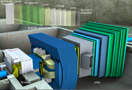
Figure 4: A simplified depiction of the MoEDAL detector, adjacent to the LHCb detector, at Point 8 on the LHC ring.

$$-\frac{dE}{dx}=K\frac{Z}{A}(ng)^{2}\left[ln\frac{2m_{e}c^{2}\beta^{2}\gamma^{2}}{I_{m}}+\frac{K(|g|)}{2}-\frac{1}{2}-B(|g|)\right]$$ (27)

where $I_{m}$ is approximated by the mean excitation energy for electric charges I. The Kazama, Yang and Goldhaber cross section correction and the Bloch correction are given by $K(|g|)$ = 0.406 (0.346) for $g$ and $2g$ and $B(|g|)$ = 0.248 (0.672, 1.022, 1.685) for $g,2g,3g,6g$ ahlen , and are interpolated linearly to intermediate values of $|g|$. The expression above is only valid only down to a velocity of $\beta\sim$0.05.

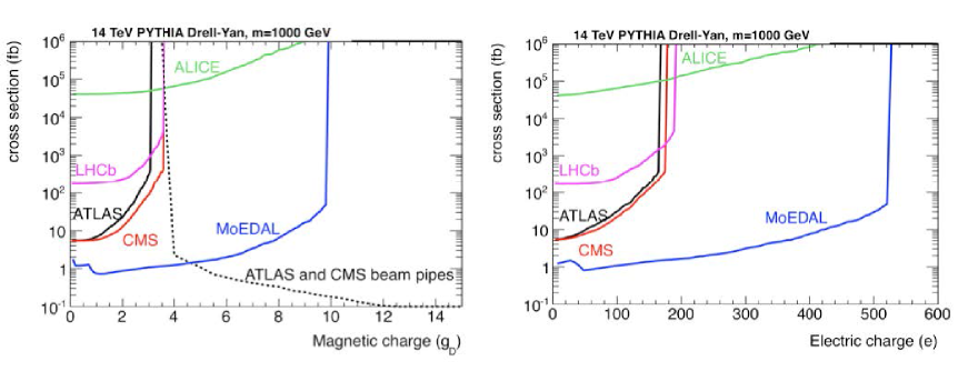
Figure 5: The expected reach of the search for the direct detection of monopole – anti-monopole pair production produced via the Drell-Yan process at the LHC (Ecm =14 TeV). It is assumed here that the luminosity taken by LHCb/MoEDAL is 2 ${\rm fb}^{-1}$, ATLAS & CMS 20 ${\rm fb}^{-1}$, and ALICE only 0.004 ${\rm fb}^{-1}$.

One key difference between a relativistic magnetic monopole with a single Dirac charge and a electrically charge particle is that the ionization of a medium caused by the monopole is very much greater than that of the electrically charged particle. For example, the ionization caused by a singly charged, highly relativistic Dirac monopole is $\sim$4700 times that of, say, a proton moving at the same speed.

However, a singly charged EW monopole has a magnetic charge of $2g$. Thus, the $dE/dx$ of a highly relativistic singly charged EW monopole is $\sim$ 18,800 (4 x 4700) times that of a highly relativistic monopole. Another important difference between electric and magnetic charge is the behaviour at low velocity. In the case of electric charge the dE/dx of the particle increases with decreasing $\beta$, giving rise to a large fraction of the particle s energy being deposited near the end of its trajectory - the so-called Bragg peak. However, in the case of magnetic charge can be the dE/dx is expected to $\it diminish$ with decreasing $\beta$.

The MoEDAL detector consists of the largest array (over 260 sqm) of plastic Nuclear Track Detector (NTD) stacks and trapping detectors ever deployed at an accelerator. MoEDAL is a largely passive detector which has a dual nature. First, as a giant camera for ”photographing” new physics where the NTD systems are the camera’s ”film” and second as a matter trap analyzer for new massive stable magnetically or electrically charged particles.

The main general purpose LHC detectors, ATLAS and CMS, are optimized for the detection of singly electrically charged particles moving near to the speed of light as well as neutral standard model particles (neutrons, photons, etc.). On the other hand MoEDAL is designed to detect electrically or magnetically charged particles with energy loss greater than or equal to around five times that of a minimum ionizing particle. As MoEDAL requires no trigger or reader electronics slowly moving particles present no problem for detection. Thus, the MoEDAL detector operates in a way that is complementary to the existing multi-purpose LHC detectors.

A relativistic electroweak monopole has a magnetic charge that is a multiple of 2n (n=1,2,3…) that of the Dirac charge - equivalent to an ionizing power of  9400n (n=1,2,3..) times that of a Minimum Ionizing Particle (MIP). Thus, it would be rapidly absorbed in the beampipe or in the first layers of the massive general purpose LHC experiments such as ATLAS and CMS, making it difficult to detect and measure. If the fundamental charge was $e/3$ instead of $e$ then the ionizing power would be nine time higher making the problem worse.

However, the full width of the MoEDAL plastic NTD detector array stacks which are at most only about 5mm thick can be traversed by magnetic monopoles with up to around six Dirac charges. In addition, the NTD stacks can be calibrated directly for very highly ionizing particles using heavy-ion beams, this is not possible with the standard LHC experiments. Once calibrated the charge resolution of an NTD stack can be as good as 1/100 of a single electric charge. A monopole traversing a MoEDAL NTD stack of 10 plastic foils would leave a trail of 20 etch pits (allowing a precise measurement of the effective charge) aligned with respect to each other to a few microns - there is no known standard model background to such a signal.

An additional strength of the MoEDAL detector is the use, for the first time at an accelerator, of purpose built trapping detectors comprised of aluminium volumes. A fraction of the very highly ionizing particles produced during collisions would be trapped in these volumes. Periodically, the trapping detectors are replaced and the exposed detectors monitored for the presence of trapped magnetic charge using a SQUID magnetometer. In this way the MoEDAL detector can be used to directly measure the magnetic charge, a first for a collider detector.

Typically the standard LHC detectors need a largish statistical sample to establish a signal and measure the basic properties of the detected particle. However, the MoEDAL detector requires only one particle to be detected in the NTD array and/or captured in the trapping detectors in order to declare discovery and to determine the basic properties of the particle. In most cases we can expect that corroborating evidence should be available from the other LHC detectors in the event of a discovery by the MoEDAL detector. The reach of the MoEDAL experiment in the physics arena where highly ionizing particles are the harbingers of new physics is shown in Fig. 5 moedal-reach .

IV Conclusion

Dirac first hypothesized the existence of the magnetic monopole in 1931 Dirac as a quantised singularity in the electromagnetic field. Since then we have had the Wu-Yang monopole wuyang , the ’tHooft-Polyakov monopole thooft , and the grand unification monopole dokos , and the quest for magnetic monopoles has continued both theoretically and experimentally. But only the electroweak, or Cho-Maison, monopole is consistent with the theoretical framework of the standard model, where the Dirac monopole becomes the Cho-Maison monopole after the electroweak unification.

The existence of the electroweak monopole invites exciting new questions. What is its spin, and how can we predict it? How can we construct the quantum field theory of monopole? What are the new physical processes induced by the monopole? What is the impact of the monopole on cosmology, particularly the cosmology of the early universe?

The MoEDAL experiment is optimized to detect very highly ionizing particles such as the Cho-Maison monopole. Indeed, a significant portion of its estimated possible mass range is accessible at the LHC. If the Cho-Maison is produced at the LHC with the expected cross-section then MoEDAL will detect it.

There is no doubt that the discovery of the Cho-Maison monopole would be comparable in importance to that of the Higgs boson and arguably more revolutionary. For example, if discovered, the Cho-Maison monopole will be the first elementary particle with magnetic charge and the first elementary particle that is topological in nature.

References

- (1) G. Aad et al. (ATLAS Collaboration), Phys. Lett. B716, 1 (2012); S. Chatrchyan et al. (CMS Collaboration), Phys. Lett. B716, 30 (2012); T. Aaltonen et al. (CDF and D0 Collaborations), Phys. Rev. Lett. 109, 071804 (2012).
- (2) Y. M. Cho and D. Maison, Phys. Lett. B391, 360 (1997); W. S. Bae and Y. M. Cho, JKPS 46, 791 (2005).
- (3) Yisong Yang, Proc. Roy. Soc. A454, 155 (1998); Yisong Yang, Solitons in Field Theory and Nonlinear Analysis (Springer Monographs in Mathematics), p. 322 (Springer-Verlag) 2001.
- (4) T. Vachaspati and M. Barriola, Phys. Rev. Lett. 69, 1867 (1992); M. Barriola, T. Vachaspati, and M. Bucher, Phys. Rev. D50, 2819 (1994).
- (5) Y. M. Cho, Kyoungtae Kim, J. H. Yoon, arXiv hep-ph 1212.3885; hep-ph 1305.1699, to be published.
- (6) M. Prasad and C. Sommerfield, Phys. Rev. Lett. 35, 760 (1975).
- (7) J. L. Pinfold, “MoEDAL -Technical Design Report”, MoEDAL Collaboration, CERN-LHC-2009-006, MoEDAL-TDR-1.1, Feb. 27, (2010). See also CERN Courier 52, No. 7, p. 10 (2012).
- (8) Particle Data Group Collaboration, Review of particle physics, J. Phys. G 37 075021 (2010).
- (9) S. Ahlen, Phys. Rev. D 17, 229 (1978).
- (10) A. De Roeck et al., Euro Phys. J. C72, 1985 (2012).
- (11) P. A. M. Dirac, Proc. Roy. Soc. (London) A133, 60 (1931).
- (12) T. T. Wu, and C. N. Yang, in Properties of Matter under Unusual Conditions, edited by H. Mark and S. Fernbach (Interscience, New York) 1968; Y. M. Cho, Phys. Rev. Lett. 44, 1115 (1980).
- (13) G. ’t Hooft, Nucl. Phys. B79, 276 (1974); A. M. Polyakov, Zh. Eksp. Teor. Fiz. Pis’ma. Red. 20, 430 (1974) [JETP Lett. 20, 194 (1974)]; B. Julia and A. Zee, Phys. Rev. D11, 2227 (1975).
- (14) C. Dokos and T. Tomaras, Phys. Rev. D21, 2940 (1980).