Turbulence model for simulation of the flame
front propagation in SNIa

Abstract

Turbulence significantly influences the dynamics of flame in SNIa. The large Reynolds number makes impossible the direct numerical simulations of turbulence, and different models of turbulence have to be used. Here we present the simulations with the $k$-$\epsilon$ model. The turbulence is generated by the RTL instability and crucially influences flame front velocity, resulting in $v_{\rm flame}\sim 300$ km/s. The model reproduces turbulent properties in low-dimensional simulations and can be used for the low-cost studies.

I Introduction

The problem of a nuclear flame propagation in the SNIa is still controversial and is one of the fundamental questions in astrophysics and the theory of burning. These flashes are considered to be the thermonuclear explosions of a white dwarf close to Chandrasekhar limit in binary systems. There exist three popular scenarios of SNIa events: single–degenerate, double–degenerate and sub–Chandrasekhar explosions (see, e.g. Hillebrandt and Niemeyer (2000)). The first depends crucially on flame physics: to meet observations it requires two stages of burning propagation, slow burning (the deflagration) and the detonation. The effective mechanism of deflagration to detonation transition (DDT) should exist Khokhlov et al. (1997); Lisewski et al. (2000); Seitenzahl et al. (2013) and is an essential part of the single–degenerate scenario considered here, when the progenitor of the explosion is a white dwarf (WD) in a binary system with a non-degenerate companion star.

The flame in conditions of a white dwarf is negligibly thin compared to any other spatial scale Timmes and Woosley (1992). Such a flame is subject to many instabilities Hillebrandt and Niemeyer (2000); Niemeyer and Woosley (1997); Glazyrin (2013). The effects of such instabilities are in changing the character of the flame propagation (like the change of its velocity) or turbulization of medium (and influence on flame through turbulence). The latter is considered in this paper. The flame velocity acceleration close to the speed of sound is an essential part of DDT and turbulence could do it effectively.

Though several effects lead to turbulization, only one instability is considered in this paper as it plays the dominating role in SNIa. This is the instability of the surface separating two mediums with different densities in gravitational field. For the non-interacting mediums it is called the Rayleigh–Taylor instability, and for flames it was first considered by Landau in Landau (1944) (the famous Landau–Darries instability was also introduced in that paper), so we will use below the term Rayleigh–Taylor–Landau instability (RTL) for flames. The surface can be unstable when density gradient and gravitational acceleration satisfy: ${\bf g}\nabla\rho<0$, what is true for a flame spreading outwards the centre of a star.

The turbulent flames in SNIa were considered in a number of papers. In the paper Niemeyer and Hillebrandt (1995) the subgrid-scale model for turbulence was implemented, the main source of turbulence was the RTL instability, as in our work. It was shown that the turbulence increases flame velocity to $\sim 2$% of the sound speed. This model of turbulence was significantly updated in papers Schmidt et al. (2006, 2006). With this new model a full 3D simulation of a star is presented in Röpke (2007). It was shown that deflagration–to–detonation transition could be fully flame driven, as there are non-negligible probabilities of turbulent velocities $v^{\prime}>10^{3}$ km/s (for details see Röpke (2007)). Another approach is presented in Woosley et al. (2009), where the authors used the sophisticated 1D semi–empirical model for turbulent flames called Linear–Eddy–Model (LEM). The authors succeeded in DDT explanation in conditions on border of two regimes of turbulent flame propagation. Also we should mention works like Aspden et al. (2008), where the microphysics of turbulence–flame interaction is considered.

We use here the semi–empirical $k$-$\epsilon$ model to calculate turbulent burning and turbulent parameters. The model accurately simulates Rayleigh–Taylor (RT) and Kelvin–Helmholtz (KH) mixing processes. The benefit of such a model is that it can correctly reproduce 3D properties of turbulence in low-dimensional simulations. In this paper the 1D model of turbulence generation by the RTL instability at the flame interface together with the impact of turbulence on the flame is considered. A similar to our model was proposed in Simonenko et al. (2007) for the problems of thermonuclear burning on a surface of neutron stars. The Section II presents the model of turbulence, the setup of the problem for WD together with numerical approach used is presented in Section III, Section IV contains results of simulations, the discussion is presented in Section V.

II The model of turbulent flame

The class of turbulence models we are using was initially proposed in paper Jones and Launder (1972). These models meet several requirements: they should reproduce Navier–Stokes equations when quantities that characterise turbulence are set to zero; and also reproduce the leading terms in Navier–Stokes equations for the Reynolds number ${\rm Re}\rightarrow\infty$. The simplest procedure to satisfy these requirements is to build a model by averaging exact hydrodynamic equations, and try to close the obtained system at some level of correlators. The considered model is a Reynolds-averaged model is contrast to large eddy simulation model by Schmidt et al. (2006), which is based on filtering.

The system of hydrodynamic equations with burning looks like:

$$\partial_{t}\rho+\partial_{i}(\rho v_{i})=0,$$ (1)

$$\partial_{t}(\rho v_{i})+\partial_{j}(\rho v_{i}v_{j})+\partial_{i}p=\partial_{j}\tau_{ij},$$ (2)

$$\partial_{t}(\rho e)+\partial_{i}\left(\rho ev_{i}\right)+p\partial_{i}v_{i}+\partial_{i}Q_{i}=\tau_{ij}\partial_{j}v_{i}+\dot{S},$$ (3)

here $\rho$ – is the density of the medium, $v_{i}$ – velocity, $p$ – pressure, $e$ – internal energy per unit mass, $\tau_{ij}$ is the viscous tensor, $Q_{i}$ – heat flow, $\dot{S}$ energy generation by flame.

We will not provide explicit expressions for $Q_{i}$ and $\dot{S}$ here as they are not required in the paper. But the dynamics of the deflagration flame for laminar flows is determined by these two processes: thermoconductivity and energy generation. If $\kappa$ is the coefficient of thermoconductivity (defined as $Q_{i}=-\kappa\partial_{i}T$), $q$ – caloricity, then the flame thickness $\delta$ satisfies

$$\frac{\delta^{2}}{\kappa}=\frac{q}{\dot{S}}=\tau_{\rm flame}.$$ (4)

This equality means that for the flame to exist the energy should be transferred through its thickness to heat the next layer on a timescale of energy generation Landau and Lifshitz (1959).

We consider the case when the burning timescale is much smaller than the turbulent and hydrodynamic one’s (further we will provide an exact criterion). It means that we can introduce the concept of flame as a thin surface that separates burned and unburned matter. In this case we can exclude the thermoconductivity from Eqns. (1)–(3). But the flame will now be moved “by hands”: we should set its normal velocity $u_{n}$ (as a function of matter state) and energy generation on the front. In general 3D case the equation that describes its dynamics reads, e.g., as Reinecke et al. (1999):

$$\partial_{t}G+(v\nabla)G=u_{n}({\bf x},t)|\nabla G|,$$ (5)

where $G({\bf x},t)$ is a level-function:

$$G<0: \quad\mbox{unburned matter},$$ (6)

$$G>0: \quad\mbox{burned matter}.$$

For such flame model its normal flame velocity should be pre-calculated in the full–physics hydrodynamic simulations like Timmes and Woosley (1992); Glazyrin et al. (2012). In the scope of this paper we use the approximation formulas from Timmes and Woosley (1992).

The turbulence is characterized by the existence of a cascade: a interval in the space of wave-numbers with a universal scaling law where energy is transferred from the large scale to the dissipation scale. The turbulent pulsations $v^{\prime}$ depend on the spatial scale $l$. We can define the Gibson scale $l_{G}$ as:

$$v^{\prime}(l_{G})=u_{n}.$$ (7)

The physical meaning of the scale is that a turbulence does not influence on a flame on spatial scales $l<l_{G}$ and affects it on scales $l>l_{G}$. The regime of turbulent burning we are considering (the flamelet regime) is described in terms of the Karlovitz number:

$${\rm Ka}\equiv\left(\frac{\delta}{l_{G}}\right)^{1/2}\ll 1.$$ (8)

To build a model of a turbulence we average hydrodynamic equations. The following rules are used. The Reynolds averaging

$$\overline{A}({\bf x},t)=\frac{1}{T}\int\limits_{-T/2}^{T/2}A({\bf x},t+\tau)d\tau,$$ (9)

where $T$ is the characteristic timescale of turbulent pulsations. For compressible fluids it is better to use the Favre averaging,

$$\tilde{A}=\frac{\overline{\rho A}}{\overline{\rho}},$$ (10)

for some quantities, namely: $v$, $e$. The other quantities, $\rho$, $p$, $\tau_{ij}$, will be averaged by Reynolds rule. Every quantity can be split into averaged and pulsational parts:

$$A=\overline{A}+A^{\prime}=\tilde{A}+A^{\prime\prime},\quad A^{\prime}=A^{\prime\prime}+\frac{\overline{\rho^{\prime}A^{\prime}}}{\overline{\rho}}.$$ (11)

The latter equality can be deduced from definitions.

After working on hydrodynamic equations we obtain (for details see Yanilkin et al. (2009); Besnard et al. (1992)):

$$\partial_{t}\overline{\rho}+\partial_{i}(\overline{\rho}\tilde{v}_{i})=0,$$ (12)

$$\partial_{t}(\overline{\rho}\tilde{v}_{i})+\partial_{j}(\overline{\rho}\tilde{v}_{i}\tilde{v}_{j})+\partial_{j}R_{ij}+\partial_{i}\overline{p}=\partial_{j}\overline{\tau}_{ij},$$ (13)

$$\partial_{t}(\overline{\rho}\tilde{e})+\partial_{i}\left(\overline{\rho}\tilde{e}\tilde{v}_{i}\right)+\partial_{i}\left(\overline{\rho e^{\prime\prime}v_{i}^{\prime\prime}}\right)+\overline{p}\partial_{i}\overline{v}_{i}+\overline{p^{\prime}\partial_{i}v_{i}^{\prime}}=\overline{\tau}_{ij}\partial_{j}\tilde{v}_{i}+\overline{\tau_{ij}\partial_{j}v^{\prime\prime}_{i}}+\overline{\dot{S}},$$ (14)

with definitions $R_{ij}\equiv\overline{\rho v^{\prime\prime}_{i}v^{\prime\prime}_{j}}$, $R_{ij..k}\equiv\overline{\rho v^{\prime\prime}_{i}v^{\prime\prime}_{j}...v^{\prime\prime}_{k}}$ ($R_{ij}$ is a Reynolds tensor, it describes the momentum transfer by turbulence).

The goal of a turbulence model is to calculate the unknown terms, second and higher order correlators of pulsational quantities, $R_{ij}$, $\overline{\rho e^{\prime\prime}v_{i}^{\prime\prime}}$, etc.

The general idea of $k$-$\epsilon$ models is to introduce two additional dynamical quantities: the energy of turbulent pulsations (here $v^{\prime\prime}$ characterises pulsations on the scale of a turbulent energy generation, compare Eq. (7) and the text above it) and its dissipation:

$$k\equiv\frac{1}{\overline{\rho}}\frac{\overline{\rho(v^{\prime\prime}_{i})^{2}}}{2},\quad\epsilon\equiv\frac{1}{\overline{\rho}}\overline{\tau_{ij}^{\prime}\partial_{j}v_{i}^{\prime}}.$$ (15)

These quantities define the turbulent timescale $\tau_{T}=k/\epsilon$. It introduces the turbulent diffusion coefficient

$$D\sim v^{\prime\prime 2}\tau_{T}\sim\frac{k^{2}}{\epsilon}.$$ (16)

The diffusion coefficient makes it possible to calculate turbulent averages $\overline{v^{\prime\prime}A^{\prime}}$ with the “gradient approximation” Belenkii and Fradkin (1965):

$$\overline{v_{i}^{\prime\prime}A^{\prime}}\sim-D\partial_{i}A.$$ (17)

When applying this approximation, different constants of proportionality are used for different physical quantities $A$.

The Reynolds tensor with this approximation (with symmetry properties) is

$$R_{ij}=-\rho D\left(\partial_{i}v_{j}+\partial_{j}v_{i}-\frac{2}{3}\delta_{ij}\partial_{l}v_{l}\right)+\frac{2}{3}\rho k\delta_{ij},$$ (18)

the first term is the turbulent viscosity, and the second one is the turbulent pressure.

Let us deduce the equation for the turbulent energy $k$. From (2) and (13) we obtain exact equation for $k$:

$$\partial_{t}(\overline{\rho}k)+\partial_{j}(\overline{\rho}\tilde{v}_{j}k)+\frac{1}{2}\partial_{j}R_{iij}+R_{ij}\partial_{j}\tilde{v}_{i}=-\overline{v_{i}^{\prime\prime}\partial_{i}p}+\overline{v_{i}^{\prime\prime}\partial_{j}\tau_{ij}}.$$ (19)

Let us concisely consider different terms in this equation: $-R_{ij}\partial_{j}\tilde{v}_{i}$ is a shear turbulence generation term $G_{1}$. Another generation term appears from

$$-\overline{v_{i}^{\prime\prime}\partial_{i}p}=-\overline{v_{i}^{\prime\prime}}\partial_{i}\overline{p}-\overline{v_{i}^{\prime\prime}\partial_{i}p^{\prime}}=\frac{\overline{\rho^{\prime}v_{i}^{\prime}}}{\overline{\rho}}\partial_{i}p-\overline{v_{i}^{\prime\prime}\partial_{i}p^{\prime}},$$ (20)

here the second term in the RHS is omitted (for low-Mach flows as is $\sim{\rm Ma}^{3}$) and the generation term is

$$G_{2}\equiv\frac{\overline{\rho^{\prime}v_{i}^{\prime}}}{\overline{\rho}}\partial_{i}p.$$ (21)

The expression $-\partial_{j}R_{iij}/2$ is approximated with the gradient rule as a diffusion term $\partial_{j}(c_{k}\rho D\partial_{j}k)$. The term $\overline{v_{i}^{\prime\prime}\partial_{j}\tau_{ij}}$ is $\rho\epsilon$ for high-Reynolds-number flows. So finally the equation for turbulent energy is (in final model equations we will drop the notation of averaging):

$$\partial_{t}(\rho k)+\partial_{i}(\rho kv_{i})=G_{1}+G_{2}-\rho\epsilon+\partial_{i}(\rho c_{k}D\partial_{i}k).$$ (22)

Analogously in Eq. (14) $\overline{\tau_{ij}\partial_{j}v_{i}^{\prime\prime}}$ is approximated as $\rho\epsilon$, terms $\overline{p^{\prime}\partial_{i}v_{i}^{\prime}}$ and $\overline{\tau}_{ij}\partial_{j}\tilde{v}_{i}$ are omitted (the first term for low-Mach flows and from the energy conservation law (see further); the second is the collisional viscosity, it is negligible in comparison with the turbulent viscosity), $\overline{\rho e^{\prime\prime}v_{i}^{\prime\prime}}$ is turbulent thermoconductivity $Q_{i}^{T}=-c_{e}\rho D\partial_{i}e$. In the term $\overline{p}\partial_{i}\overline{v}_{i}$ the velocity should be replaced by Favre average with Eq. (11), it leads to additional term $\partial_{i}(pa_{i})$ in the final equation ($a_{i}\equiv\overline{\rho^{\prime}v^{\prime}}/\overline{\rho}$). We should note that the final variant of the equation for internal energy $e$ should be consistent with the equation for $\rho v^{2}/2$ and $\rho k$ to conserve energy, what is true with proposed earlier approximations.

The exact equation for $\epsilon$ contains a lot of complex terms that are not easily approximated in the considered framework, so usually it is written similar to $k$-equation:

$$\partial_{t}(\rho\epsilon)+\partial_{i}(\rho\epsilon v_{i})=\frac{\epsilon}{k}\left(c_{\epsilon 1}G_{1}+c_{\epsilon 2}G_{2}-c_{\epsilon 3}\rho\epsilon\right)+\partial_{i}(\rho c_{\epsilon}D\partial_{i}\epsilon),$$ (23)

The proposed procedure of “derivation” should not be considered as rigorous, the general aim of it was to show the correspondence between terms of exact averaged hydrodynamic equations and model terms. For more details see Yanilkin et al. (2009); Besnard et al. (1992).

The full system of the model of turbulence (hereafter we drop the notation of averaging):

$$\partial_{t}\rho+\partial_{i}(\rho v_{i})=0,$$ (24)

$$\partial_{t}(\rho v_{i})+\partial_{j}\left(\rho v_{i}v_{j}+p\delta_{ij}\right)=-\partial_{j}R_{ij},$$ (25)

$$\partial_{t}E+\partial_{i}(v_{i}(E+p))=-G_{2}+\rho\epsilon+\partial_{i}(pa_{i}-Q_{i}^{T}),$$ (26)

$$R_{ij}=-\rho D\left(\partial_{i}v_{j}+\partial_{j}v_{i}-\frac{2}{3}\delta_{ij}\partial_{k}v_{k}\right)+\frac{2}{3}\rho k\delta_{ij},$$ (27)

$$\partial_{t}(\rho k)+\partial_{i}(\rho kv_{i})=G_{1}+G_{2}-\rho\epsilon+\partial_{i}(\rho c_{k}D\partial_{i}k),$$ (28)

$$\partial_{t}(\rho\epsilon)+\partial_{i}(\rho\epsilon v_{i})=\frac{\epsilon}{k}\left(c_{\epsilon 1}G_{1}+c_{\epsilon 2}G_{2}-c_{\epsilon 3}\rho\epsilon\right)+\partial_{i}(\rho c_{\epsilon}D\partial_{i}\epsilon),$$ (29)

$$E=\rho e+\frac{\rho v^{2}}{2},\quad D=c_{D}\frac{k^{2}}{\epsilon},\quad a_{i}=-c_{\alpha}D\frac{\partial_{i}\rho}{\rho},$$ (30)

$$G_{1}=-R_{ij}\partial_{i}v_{j},\quad G_{2}=a_{i}\partial_{i}p,\quad Q_{i}^{T}=-c_{e}\rho D\partial_{i}e.$$ (31)

One of the main weakness of the model are the unknown constants. The procedure of model derivation does not fix the constants. There are several ways to obtain their values: comparison with experiments, the direct numerical simulation Guzhova et al. (2005), some theoretical approaches like renorm–group Yakhot and Orszag (1986). In this work the following set of constants is used Guzhova et al. (2005): $c_{\alpha}=1.7$, $c_{D}=0.12$, $c_{e}=3$, $c_{\epsilon 1}=1.15$, $c_{\epsilon 2}=1$, $c_{\epsilon 3}=1.7$, $c_{k}=c_{\epsilon}=4/3$ (the model with the set of constants was tested upon several laboratory experiments: Rayleigh–Taylor mixing experiments Dimonte and Schneider (2000), Kelvin–Helmholtz mixing experiments Browand and Latigo (1979), and direct numerical simulations of these processes Guzhova et al. (2005); the full list of experiments is presented in Guzhova et al. (2005)).

To finish the model for burning we should add the influence of the turbulence on flame (flame influences turbulence by generating gradients of quantities). It is done in our work by changing the flame velocity. In the regime when (8) is satisfied (the flamelet regime), the effect of turbulence exhibits itself only in curvature of flame surface. Such regime was considered in the paper Yakhot (1988) (see also Kerstein (1988)) with a renorm–group analysis. The result could be written as:

$$\frac{v_{\rm turb}}{v_{\rm lam}}=\exp\left(\frac{2k}{v_{\rm turb}^{2}}\right),$$ (32)

where $v_{\rm lam}$ – is a laminar speed (from Timmes and Woosley (1992)), $v_{\rm turb}$ – a turbulent flame speed. The proposed expression is pure theoretical, though it was tested on some experimental data (see Yakhot (1988)), it may need additional consideration.

III The problem setup

We consider a white dwarf close to the Chandrasekhar limit $M_{\rm Ch}$. We are interested in the process of a flame propagation from the centre to outer regions of the WD: according to evolutionary star models the flame is born near the centre and, to meet observations, it should over time transform to the detonation wave Hillebrandt and Niemeyer (2000). The slow burning (flame) leads to expansion of matter, therefore in the region near the flame the conditions of RTL instability growth are satisfied. On the characteristic global timescale of flame propagation (here we mean $\sim R_{\rm WD}/u_{n}$, not (4)), RTL manages to evolve to the nonlinear stage and develop turbulence. We are interested in its intensity and its impact on the flame.

To answer these questions we use numerical simulations. Equations (24)–(31) are implemented in our numerical hydrocode FRONT3D fro in three-dimensional case. As was mentioned earlier, the model of turbulence can correctly reproduce 3D properties of turbulence even in 1D simulations. Therefore to see the magnitude of the turbulence effect we work in 1D spherical coordinates in the scope of this paper. Not to encounter the problem of building equilibrium WD configuration in Eulerian code, we implemented a lagrangian 1D numerical scheme as a module in FRONT3D code for one-dimensional simulations. We use an implicit scheme in mass coordinates proposed in Samarskii and Popov (1992) (the scheme contains the artificial viscosity for shock wave problems, but our flows are significantly subsonic, so it have no effect for our problem; furthermore, turbulence leads to the appearance of the turbulent viscosity in our model, this turbulent viscosity in much greater than artificial). This scheme uses staggered mesh: coordinate and velocity are set at boundaries of cells $r_{i}$, $v_{i}$ and other quantities in the centres of cells $p_{i+1/2}$, $\rho_{i+1/2}$ etc. Details of the implementation can be found in the documentation that goes with the code. The turbulent terms in hydrodynamic equations are included in this scheme as external sources.

To treat correctly the properties of medium in the WD we use “Helmholtz” tabular equation of state Timmes and Swesty (2000). The initial distributions of all parameters are set to hydrodynamic equilibrium with a numerical precision by the following procedure. The distribution of mass $m_{i}$ and central density $\rho_{c}$ are set as a first step. Then the recursive procedure determines profiles in the star:

$$4\pi r_{i}^{2}\frac{p_{i+1/2}-p_{i-1/2}}{\Delta m_{i}}=-\frac{Gm_{i}}{r_{i}^{2}},$$ (33)

$$\rho_{i+1/2}={\rm EOS}(p_{i+1/2},T_{i+1/2}),$$ (34)

$$r_{i+1}^{3}=r_{i}^{3}+\frac{3}{4\pi}\frac{\Delta m_{i+1/2}}{\rho_{i+1/2}}.$$ (35)

This procedure requires the known $T(\rho,r)$ dependence. The temperature after burning raises significantly, up to $\sim 10^{10}$ K, we could use any small temperature as initial. Because thermoconductivity in WD is strong, the star is usually isothermal in the centre. After all this, we set constant $T_{\rm initial}$ everywhere. The choice of $T_{\rm initial}$ is presented below. After integration we obtain the state of the WD close to the Emden solution, but in equilibrium with the “real” EOS.

The Eq. (5) describes evolution of flame surface for general situation. For our case there exist much simpler procedure to consider burning. The flame is defined by its position in mass coordinates: $m_{\rm flame}$. The evolution of its coordinate satisfies the equation:

$$\frac{dm_{\rm flame}}{dt}=4\pi r_{\rm fl}^{2}\rho v_{\rm fl},$$ (36)

where $r_{\rm fl}$ is the current position of flame, $\rho$, $v_{\rm fl}$ – the density and the flame velocity (as a function of medium state) at this point. On every step energy released by burning is $\Delta Q=q\Delta m$, $\Delta m$ is the mass of matter burned on the timestep (this energy is spread on cells the flame moves throw). The flame is initially set as a point $m_{\rm ign}$, from which two fronts (forward and backward) start to propagate. The flame velocity is calculated solving the implicit equation (32) on each time-step in our code for each flame front.

IV Results

Here we present the results of simulations. The parameters of the initial white dwarf are set as: the central density $\rho_{c}=2\times 10^{9}$ g/cm³, the initial composition as pure ¹²C or the mixture 0.5¹²C+0.5¹⁶O. The initial temperature is calculated with the approximation for the ignition curve from Potekhin and Chabrier (2012): for ¹²C it is $T_{\rm initial}=2.7\times 10^{8}$ K, for 0.5¹²C+0.5¹⁶O it is $T_{\rm initial}=3.8\times 10^{8}$ K (both temperatures are much smaller than the temperature after burning $\sim 5\times 10^{9}$ K, what corresponds the statement from previous section). We present results for several variants of the caloricity: $q_{1}=5.6\times 10^{17}$ erg/g (corresponds to transition C$\rightarrow$Mg), $q_{2}=9.2\times 10^{17}$ erg/g (C$\rightarrow$Ni), and intermediate $q_{3}=7\times 10^{17}$ erg/g (corresponds to transition to the NSE for carbon burning Niemeyer and Hillebrandt (1995)). With such variants of we overlap a wide range of $q$ and check the dependence of results on it. The conditions of convection preceding ignition are presented in the paper Nonaka et al. (2012): our flame is ignited at the point with $r_{\rm ign}=50$ km, initial turbulent velocity $v_{0}^{\prime\prime}=\sqrt{2k_{0}}=16$ km/s, and the turbulent length $L_{\rm turb}=k_{0}^{3/2}/\epsilon_{0}=200$ km.

The example of density evolution vs time is shown in Fig. 1. The density drop, generated by flame spreading outwards, is smoothed by the turbulence appeared.

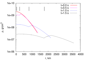
Figure 1: Density profiles for different moments, the variant with $q=9.2\times 10^{17}$ erg/g, ¹²C initial. Vertical marks show positions of the flame for these moments of time

The latter is maintained by the RTL instability, which growth is proportional to the gravitational acceleration at the location of the flame:

$$g_{\rm fl}=\frac{Gm_{\rm flame}}{r_{\rm flame}^{2}}.$$ (37)

Flame position $m_{\rm flame}$ grows with time together with $r_{\rm flame}$, the cumulative effect of the instability yield is unknown a priori. The profiles of specific turbulent energy for the same simulation as in Fig. 1 are shown in Fig. 2.

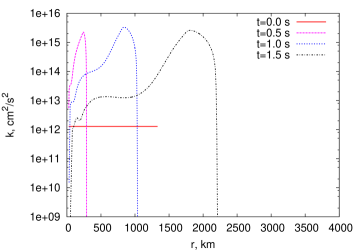
Figure 2: Turbulent energy profiles for different moments, the variant with $q=9.2\times 10^{17}$ erg/g, ¹²C initial

It could be seen that the maximum energy $\sim 2\times 10^{15}$ erg/g (for the considered variant of initial conditions) is maintained with time near the current position of the flame. This intensive turbulence that exceeds background initial values is generated very early. That is why the effect of changing initial turbulent quantities $k_{0}$, $L_{0}$ have very small effect on the results, this fact will be explicitly tested further, and shows the correctness of the model work. The resulting turbulent velocities of flame fronts for all variants are shown in Fig. 3.

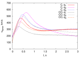
(a)

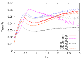
(b)

Figure 3: Flame velocities (on the left) and the Mach numbers (on the right) for all variants

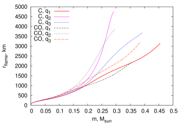
Figure 4: Positions of the flame front versus massive coordinates for all variants

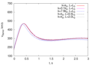
Figure 5: Flame velocities for the variant with ¹²C and $q=q_{1}$ with various initial turbulent parameters $k_{0}$ and $L_{0}$

The increase of velocity that occurs at early times is connected with the raise of turbulent energy (without the turbulent impact the velocity will monotonically decrease). Flame velocity satisfies $v_{\rm flame}\approx\sqrt{2k}$ almost all the time, that is why more precise relation instead of (32) is not required in these simulations, together with more exact $u_{n}(\rho,X_{i})$ dependence. It could be seen that turbulence maintains flame velocity on the level of (200-300) km/s, that is $\sim$ (3-7)% of the sound speed, what is much smaller than the latter and shows that this turbulent regime does not lead to DDT. The Fig. 4 show the position of flame front versus massive coordinate for all variants. It could be seen that larger caloricity leads to faster expansion. Relatively large velocity of turbulent flame maintains active burning till the end of simulation, when $\rho$ drops to several $10^{6}$ g/cm³.

Additional runs were made with increased (or decreased) values of $k_{0}$, $L_{\rm turb_{0}}$ (what correspond to the variation of initial turbulence), showing the independence of final turbulence on the variation of initial and background values, see Fig. 5.

V Conclusions

The paper considers the problem of a white dwarf burning with account for turbulence. The core of the approach is a $k$-$\epsilon$ model of turbulence, which succeeds in turbulence simulations in any dimension: 1-, 2-, 3D, reproducing correctly 3D turbulence properties. Using this approach we presented 1D simulations of a white dwarf for ${\rm Ka}\ll 1$ regime of turbulent burning (the flamelet regime). As a result the stationary turbulent intensity arises after some time in simulations. This turbulence maintains flame velocity at $v_{\rm flame}\approx(250\pm 50)$ km/s. The obtained turbulent velocities agree with the results of more sophisticated simulations like Röpke (2007). The flame acceleration (the final Mach number) $\sim 0.05c_{s}$ is small and we can conclude, similar to Woosley et al. (2009), that deflagration to detonation transition occurs in different regime of turbulent burning (not in the flamelet), or on the border of two regimes (there could be identified three regimes of turbulent burning – the flamelet, the stirred flame, the well-stirred flame, for additional details see Woosley et al. (2009)) of turbulent flame propagation. It is important to note that this conclusion refers to the whole flame, according to Röpke (2007); Schmidt et al. (2010) the detonation can be triggered by rare high-velocity turbulent fluctuations. Such fluctuations are not reproduced by the proposed model correctly, it needs some modifications.

This work is planned to be continued with simulations in higher dimensions – 2D, 3D, studying of other regimes of turbulent flame, implementation of more sophisticated model of nuclear reactions, and comparison with observations. Also the considered model was tested upon terrestrial experiments on turbulent mixing (see the Section II), the question of its application for SNIa turbulence is not fully clear and should be considered further. Nevertheless such type of a model have benefits in reproducing turbulent properties in lower dimensional simulations and could be used for the low-cost studies.

The author is grateful to S. Blinnikov, F. Röpke for discussions, an anonymous referee for very valuable comments. The work is also supported by RFBR grants 11-02-00441-a and 13-02-92119, Sci. Schools 5440.2012.2, 3205.2012.2 and 3172.2012.2, by the contract No. 11.G34.31.0047 of the Ministry of Education and Science of the Russian Federation, and SCOPES project No. IZ73Z0-128180/1.

References

- Hillebrandt and Niemeyer (2000) W. Hillebrandt and J. C. Niemeyer, Annual Review of Astronomy and Astrophysics 38, 191 (2000), eprint arXiv:astro-ph/0006305.
- Khokhlov et al. (1997) A. M. Khokhlov, E. S. Oran, and J. C. Wheeler, The Astrophysical Journal 478, 678 (1997), eprint arXiv:astro-ph/9612226.
- Lisewski et al. (2000) A. M. Lisewski, W. Hillebrandt, and S. E. Woosley, The Astrophysical Journal 538, 831 (2000), eprint arXiv:astro-ph/9910056.
- Seitenzahl et al. (2013) I. R. Seitenzahl, F. Ciaraldi-Schoolmann, F. K. Röpke, M. Fink, W. Hillebrandt, M. Kromer, R. Pakmor, A. J. Ruiter, S. A. Sim, and S. Taubenberger, MNRAS 429, 1156 (2013), eprint 1211.3015.
- Timmes and Woosley (1992) F. X. Timmes and S. E. Woosley, The Astrophysical Journal 396, 649 (1992).
- Niemeyer and Woosley (1997) J. C. Niemeyer and S. E. Woosley, The Astrophysical Journal 475, 740 (1997).
- Glazyrin (2013) S. I. Glazyrin, Astronomy Letters 39, 221 (2013).
- Landau (1944) L. D. Landau, ZhETF 14, 240 (1944).
- Niemeyer and Hillebrandt (1995) J. C. Niemeyer and W. Hillebrandt, The Astrophysical Journal 452, 769 (1995).
- Schmidt et al. (2006) W. Schmidt, J. C. Niemeyer, and W. Hillebrandt, Astronomy and Astrophysics 450, 265 (2006).
- Schmidt et al. (2006) W. Schmidt, J. C. Niemeyer, W. Hillebrandt, and F. K. Röpke, Astronomy and Astrophysics 450, 283 (2006), eprint arXiv:astro-ph/0601500.
- Röpke (2007) F. K. Röpke, The Astrophysical Journal 668, 1103 (2007), eprint 0709.4095.
- Woosley et al. (2009) S. E. Woosley, A. R. Kerstein, V. Sankaran, A. J. Aspden, and F. K. Röpke, The Astrophysical Journal 704, 255 (2009), eprint 0811.3610.
- Aspden et al. (2008) A. J. Aspden, J. B. Bell, M. S. Day, S. E. Woosley, and M. Zingale, The Astrophysical Journal 689, 1173 (2008), eprint 0811.2816.
- Simonenko et al. (2007) V. A. Simonenko, D. A. Gryaznykh, N. G. Karlykhanov, V. A. Lykov, and A. N. Shushlebin, Astronomy Letters 33, 80 (2007).
- Jones and Launder (1972) W. P. Jones and B. E. Launder, International Journal of Heat and Mass Transfer 15, 301 (1972).
- Landau and Lifshitz (1959) L. D. Landau and E. M. Lifshitz, Fluid Mechanics (Pergamon Press: Oxford, 1959).
- Reinecke et al. (1999) M. Reinecke, W. Hillebrandt, J. C. Niemeyer, R. Klein, and A. Gröbl, Astronomy and Astrophysics 347, 724 (1999), eprint arXiv:astro-ph/9812119.
- Glazyrin et al. (2012) S. I. Glazyrin, S. I. Blinnikov, and A. D. Dolgov, ArXiv e-prints (2012), eprint 1208.4038.
- Yanilkin et al. (2009) Y. V. Yanilkin, V. P. Statsenko, and V. I. Kozlov, Mathematical modelling of turbulent mixing in compressible mediums (Sarov, RFNC-VNIIEF, 2009).
- Besnard et al. (1992) D. Besnard, F. Harlow, R. Rauenzahn, and C. Zemach, Tech. Rep. LA-12303-MS, Los Alamos (1992).
- Belenkii and Fradkin (1965) C. Z. Belenkii and E. S. Fradkin, Trudi FIAN 29, 207 (1965).
- Guzhova et al. (2005) A. R. Guzhova, A. S. Pavlunin, and V. P. Statsenko, VANT TPF 3, 37 (2005).
- Yakhot and Orszag (1986) V. Yakhot and S. A. Orszag, Journal of Scientific Computing 1, 3 (1986).
- Dimonte and Schneider (2000) G. Dimonte and M. Schneider, Physics of Fluids 12, 304 (2000).
- Browand and Latigo (1979) F. K. Browand and B. O. Latigo, Physics of Fluids 22, 1011 (1979).
- Yakhot (1988) V. Yakhot, Combustion Science and Technology 60, 191 (1988).
- Kerstein (1988) A. R. Kerstein, Combustion Science and Technology 60, 163 (1988).
- (29) http://dau.itep.ru/sn/front3d.
- Samarskii and Popov (1992) A. A. Samarskii and Y. P. Popov, Finite-difference methods for solving hydrohynamical problems (Nauka, 1992).
- Timmes and Swesty (2000) F. X. Timmes and F. D. Swesty, The Astrophysical Journal Supplement Series 126, 501 (2000).
- Potekhin and Chabrier (2012) A. Y. Potekhin and G. Chabrier, Astronomy and Astrophysics 538, A115 (2012), eprint 1201.2133.
- Nonaka et al. (2012) A. Nonaka, A. J. Aspden, M. Zingale, A. S. Almgren, J. B. Bell, and S. E. Woosley, The Astrophysical Journal 745, 73 (2012).
- Schmidt et al. (2010) W. Schmidt, F. Ciaraldi-Schoolmann, J. C. Niemeyer, F. K. Röpke, and W. Hillebrandt, The Astrophysical Journal 710, 1683 (2010), eprint 0911.4345.