Holographic superconductors with Weyl Corrections via gauge/gravity duality

Abstract

In this paper, we analytically compute the basic parameters of the p-wave holographic superconductors with Weyl geometrical corrections using the matching method. The explicit correspondence between the critical temperature $T_{c}$ and the dual charge density $\rho$ has been calculated as $T_{c}\propto\rho^{\frac{1}{3}}$ and the dependence of the vacuum expectation value for the dual condensate operator $\cal{O}$ on the temperature has been found analytically in the form $\langle{\cal O}_{+}\rangle\propto T_{c}^{\frac{3}{2}}T^{\Delta-\frac{1}{2}}\sqrt{1-(\frac{T}{T_{c}})^{3}}$. The critical exponent $\frac{1}{2}$ is an universal quantity according to predictions of the mean field theory and independent from the Weyl coupling $\gamma$. Our analytical results confirm the numerical results and also agree on computations using by the variational method.

I General remarks on gauge-gravity duality

Maldacena discovered direct relation between a typical coformal field theory which is invariance under conformal metric transformations on the boundary, and a gravitational description of a higher dimension model. This is the simplest interpretation of that so called anti de Sitter/conformal field theory (AdS/CFT) correspondence conjecture maldacena . As a brief review, we mention the physical basis for this conjecture which has a vital role in our paper. Firstly, we discuss conformal field theory (CFT). By CFT, we mean a quantum field theory which in it’s Hamiltonian form remains conformal invariant under metric transformations as:

$$g_{\mu\nu}\rightarrow\Omega(x)g_{\mu\nu}.$$ (1)

Now consider a general transformation of local coordinate $x^{\mu}$ as the following:

$$x^{\mu}\rightarrow x^{\mu}+u^{\mu}.$$ (2)

Here $u^{\mu}$ is composed of three parts; boost, rotation (Lorentz) and scaling. The quantum current vector is the solution of the vector equation $T^{\mu\nu}u_{\nu}=J^{\mu}$, where $T^{\mu\nu}$ is CFT energy momentum tensor. The conformal field theory energy momentum tensor has zero trace, it means $T^{\mu}_{\mu}=0$ due to the conservation law $\partial_{\mu}J^{\mu}=0$. Moreover, it satisfies a local conservation law. One of the most popular usage of AdS/CFT is a way to compute the central charge which is an efficient tool for counting degree of freedoms of the CFT. Three kinds of the generators have beeb defined associated with conformal transformations: boost, rotation and scaling or dilatation ones. The last one, dilatation operator denoted by $D$ is generator of scale transformations. It acts on any arbitrary unitary operator of CFT in the form of $D\mathcal{O}=\Delta\mathcal{O}$. Scale invariant quantum theories are the end point of the renormalization group flows. Under scaling transformations the CFT operator $\mathcal{O}$ transforms to the new one $\hat{\mathcal{O}}=\lambda^{D}\mathcal{O}(\lambda x)$.

Operators in CFT are divided into three classes: relevant to the operator appears in the CFT Hamiltonian $H_{CFT}$ and irrelevant and marginal ones that they don’t appear in the $H_{CFT}$. The key point of the CFT is that we use the relevant operators on the boundary $\hat{\mathcal{O}}$ to form the renormalizable $H_{CFT}$. In this case we can write the action of a typical field theory as the following:

$$S=S_{free}+\int d^{d+1}x\Sigma_{i}g_{i}\hat{\mathcal{O}}_{i}.$$ (3)

Here, the first term is the action formed by the free fields and the integral part contains all interactions and $g_{i}$ denotes the coupling constants. By renormalization scheme, we mean the coupling constants $g_{i}=g_{i}(\epsilon)$ satisfies the following integrable system of differential equations:

$$\frac{dg_{i}}{d\log\epsilon}=\beta_{i}(g_{j}).$$ (4)

The above equation defines the family of renormalization group (RG) flow equations.

Fixed points of the system are the critical points in which $\beta_{i}(g^{*}_{j})=0$. The main property of these fixed points is at these points the quantum theories become scale invariant and the unique quantum description of the system is a quantum field theory in which it remains invariance under conformal transformations, i.e. CFT. If we perturb CFT we induce another RG flow. In other language, AdS/CFT relates a gauge theory on the boundary with dimension $d$, described by a CFT to gravity theory of matter fields plus black holes in $d+1$ dimension. So, by gauge gravity we mean

$$\emph{Gravity}\sim\emph{CFT}$$ (5)

The above equivalence is valid in the t’Hooft large coupling limit in which we assume that the coupling of the Yang-Mills field $g_{YM}^{2}N\rightarrow\infty$. We use gauge-gravity duality via AdS/CFT when the field theories be very strongly coupled. For finite coupling corrections in the bulk, we need a full string theory.

In the language of the statistical physics of thermodynamic systems in thermal equilibrium,there is a simple but very deep relation between partition function of CFT and the total action of gravity in bulk. It summarizes as the following relation:

$$Z_{CFT}=e^{-S_{g}}$$ (6)

Here $S_{g}$ is the gravitational (Euclidean) action (AdS). Moreover, $Z_{CFT}$ denotes the partition function of the quantum fields calculated by CFT. The gravity action $S_{g}$ must be renormalized in the bulk to avoid the divergences. By using the statistical approach ,it is adequate to identify the temperature of the gravity (bulk), which is black hole temperature as the temperature of CFT, so:

$$T_{BH}=T_{CFT}$$ (7)

By definition a holographic superconductor is a superconducting system under second order phase transition which has a gravity dual model, via AdS/CFT. The most simplest case is a model of scalar field $\phi$ with the following action:

$$S\sim\int d^{4}x\sqrt{-g}\Big{(}\mathcal{L}_{CFT}+\mathcal{L}_{m}\Big{)}$$ (8)

Here $\mathcal{L}_{CFT}=R+6$ in units of $l_{AdS}=1$. When we add extra fields with $\mathcal{L}_{m}$ they induce relevant operators in the field theory at the asymptotic AdS boundary. This deformation of the field theory induce an RG flow. Now the full Hamiltonian of the CFT system by counting the relevant operators represented by:

$$\tilde{H}=H_{CFT}+\lambda_{r}\mathcal{O}_{r}+\lambda_{i}\mathcal{O}_{i}$$ (9)

Here operators identifies the fields through their expectation values, in the asymptotic forms as the following:

$$\phi=\lambda_{r}r^{d-\Delta_{\mathcal{O}_{r}}}+<\mathcal{O}_{r}>r^{-\Delta_{\mathcal{O}_{r}}}+..$$ (10)

$$\psi=\lambda_{i}r^{d-\Delta_{\mathcal{O}_{i}}}+<\mathcal{O}_{i}>r^{-\Delta_{\mathcal{O}_{i}}}+..$$ (11)

The key point is that here for relevant operators always $<\mathcal{O}_{r}>\sim\sqrt{T_{c}-T}$ which is the same as the prediction of effective models of superconductors. So, by gauge gravity we able to compute the correspondence quantities.

In condensed matter different aspects of this duality investigated condencesd1 ; condencesd2 . If the gravity part is Einstein gravity, we have a superconducting phase super1 ; super2 . To study holographic superconductors we must study black holes in an asymptotically AdS spacetimes and their gravitational duals. In low temperature limit, an instability happens and it results in a breaking of the symmetry and the final state is a holographic superconductor using dual description.

By curvature corrections, we have different higher order corrected superconductors GR1 ; GR2 ; GB1 ; GB2 ; GB3 ; GB4 ; GB5 ; HL1 ; HL2 ; wen1 ; wen2 ; epl1 ; born1 ; born2 ; cs ; maxwell ; maxwell2 ; cai2012 . Also, if the relevant operators be a vector, we have p-wave holographic superconductors pwave1 ; pwave2 ; pwave3 . Very recently we prposed a consistence model for holographic superconductors in F(R) gravity as the gravity theory in bulk F(R) . Recently, some papers have discussed the existence of the D-wave holographic superconductors d-wave1 -d-wave5 .

To solve the field equations analytically, the first pioneering work was done by Hertzog herzog . Analytical methods are perturbationherzog ; kanno , the Sturm-Liouville variational method analytic1 ; analytic2 ; ijtp ,the Matching methodGB2 .
In the present work, we focus only on Weyl corrections to p-wave holographic superconductors with the Weyl’s coupling value $-\frac{1}{16}<\gamma<\frac{1}{24}$ (see Refs.mpla -weyl ).

Our paper is written as follows: In section 2, we present a toy model for the $3+1$ dimensional holographic superconductor. Section 3, is devoted to the existence of superconducting phase. In section 4, we present analytical properties of this type of superconductors. Conclusions and discussions follow in section 5.

II p-wave superconductors with Weyl corrections

Before study the effects of Weyl coupling on p-wave holographic superconductors we want to clarify more the topic of holographic superconductors via AdS/CFT. As we mentioned before the Maldacena conjecture relates the solutions of type IIB superstring theory in $AdS_{5}\times S^{5}$ to the solutions of a super Yang-Mills theory in a four dimensional spacetime. The equivalence is valid only as a limiting case of large t’Hooft coupling . Further in the limit of large numbers of colors and these two quantities are related according to the fundamental equation $\lambda=g_{YM}^{2}N$. In fact, the extra part of the manifold $AdS_{5}\times S^{5}$ must be compact. It means a four (five) dimensional action is indeed the result on integration over a ten or eleven dimensional spacetime $AdS_{5}\times S^{5}$. If we use a noncompact of geometry instead of $S^{5}$ then the classical geometry has AdS as boundary. The role of filed theory (CFT) is how to read the quantities (expectation values of the dual operators on boundary) through an isomorphic map between these operatoes and the bulk fields, namely $\Psi$. The direct and important explicit result is the vacuum expectation value of such dual quantum operators which is equal to the two point functions of the bulk scalar field on $AdS_{5}$.

Just for more better illustration, remembering that the isomorphism is one to one map between any asymptotic value of the bulk field and a relevant operator in a gauge invariant field theory in boundary $<\mathcal{O}_{i}>$. It means also for any expression of energy momentum tensor of a typical CFT, there is only one unique geometrical structure of metric $g_{\mu\nu}$ in bulk. This is a gauge/gravity duality conjecture. Due to the dynamical approach, we have an equivalence relation between on-shell value of the total action of fields in the bulk, super string theory of gravity and the action of CFT. Here on-shell means if we compute the string action with the classical solutions of field equations, such equivalence appears. Just to recall the main idea, we consider here again the type IIB string (super) theory and it’s quantum field theoretical description via four dimensional CFT. Because, we will use the concepts of asymptotic value of scalar field as the vacuum expectation of the CFT operators, here is very usefull to re calculate explicitly relation between bulk scalar fields two point functions and expectation value of CFT operators. The computation starts by solving the scalar field equation of motion for a point like source in the $AdS_{5}$ spacetime:

$$(\nabla_{\mu}\nabla^{\mu}-m^{2})\psi=0.$$ (12)

Here, mass $m^{2}$ as we will observe, is a code for the asymptotic behavior of the field and also $<\mathcal{O}_{i}>$. In a simple $AdS_{5}$ background, the propagator reads as the following, as we can find in many references:

$$G(r;x,x^{\prime})=\frac{\Gamma(\Delta)}{\pi^{2}\Gamma(\Delta-2)}(\frac{L^{2}}{r})^{\Delta}((\frac{L^{2}}{r})^{2}+|x-x^{\prime}|^{2})^{-\Delta}.$$ (13)

As usual $x^{\prime}$ denotes retarded coordinate. The key object here is the following relation between $\Delta$ and $m^{2}$:

$$\Delta(\Delta-4)=m^{2}L^{2}.$$ (14)

The above equation as many people wrote has two positive roots but usually people take the case of $\Delta>2$. In fact from unitarity $1<\Delta<4$ and in this case, the scalar mass is bounded in the BF region.

Now if we expand Green function near the AdS boundary in which $r\rightarrow\infty$ we have:

$$G(r;x,x^{\prime})\sim\alpha(x)(rL^{-2})^{\Delta-4}+\beta(x)(rL^{-2})^{-\Delta}.$$ (15)

Here as we can check directly, the first function $\alpha$ is the source of the scalar field $\psi$ evaluated on AdS boundary and the second $\beta(x)$ is the vacuum expectation value computed for the dual operator $\mathcal{O}_{i}$. We are free to choice how we quantize the operator and it means how we fix the constant factors. In the holographic superconductors if we fix the form of the operator (s-wave,p-wave,..) depending on the form of the condensator, then our main goal is ”‘how we compute $\beta(x)$ and also $\alpha(x)$”’. By first we will have the expression of the condensation $<\mathcal{O}>$. If we put this solutions as on-shell in the bulk action and doing simple algebra and because we know the action of string and CFT are the same so we can conclude that two point function is exactly the same as the kernel of scalar field in bulk. Here it is needed to identify the color number in terms of the Newton;s gravitational constant and AdS radius.

After this brief mini review of applied AdS/CFT technique we proceed our plan to study p-wave holographic superconductors . We take the action of a p-wave superconductor in the following form epl2 :

$$S=\int dtd^{4}x\sqrt{-g}\{\frac{1}{16\pi G_{5}}(R+12)-\frac{1}{4g^{2}}F^{a}_{\mu\nu}F^{a\mu\nu}+\gamma C^{\mu\nu\rho\sigma}F^{a}_{\mu\nu}F^{a}_{\rho\sigma}\}.$$ (16)

The bulk action here is five dimensional integral. We have also $G_{5}$ as gravitational coupling . We set the AdS radius $L=1$. The field strength components $F^{a}_{\mu\nu}$ are computed using $A_{\mu}^{a}$’s (non-Abelian gauge fields):

$$F^{a}_{\mu\nu}=2\partial_{[\mu}A^{a}_{\nu]}+\varepsilon^{abc}A^{b}_{\mu}A^{c}_{\nu},\{a=1,2,3,\mu=0,1,2,3\}.$$ (17)

We introduce the non zero Weyl’s coupling $\gamma$ which is a constant and it is limited inside the interval $-\frac{1}{16}<\gamma<\frac{1}{24}$.

To fix the unique geometry on bulk and as an attempt to find the dual CFT operator’s expectation values, we take the metric as an asymptotic $AdS_{5}$ background:

$$ds^{2}=r^{2}(-fdt^{2}+dx^{i}dx_{i})+\frac{dr^{2}}{r^{2}f},\ \ i=1,2,3.$$ (18)

Here the metric function is:

$$f=1-(\frac{r_{+}}{r})^{4}.$$ (19)

The horizon coincides on $r=r_{+}$. The black hole temperature which is the same as CFT temperature, due to the simple equivalence between two different free energies of two configurations, reads as $T=\frac{r_{+}}{\pi}$. The full system of field equations areweyl :

$$\nabla_{\mu}\left(F^{a\mu\nu}-4\gamma C^{\mu\nu\rho\sigma}F^{a}_{\rho\sigma}\right)=-\epsilon^{a}_{bc}A^{b}_{\mu}F^{c\mu\nu}+4\gamma C^{\mu\nu\rho\sigma}\epsilon^{a}_{bc}A^{b}_{\mu}F^{c}_{\rho\sigma}.$$ (20)

Now to explain the superconductivity in the p-wave discipline we take the Yang-Mills gauge field in the form of a two component one form which is homogeneity but anisotropic: gauge :

$$A=\phi(r)\sigma^{3}dt+\psi(r)\sigma^{1}dx.$$ (21)

As usual $\sigma^{i}$ denotes Pauli’s matrixes. The resulting field equations Yang-Mills (18) are as the following:

$$\left(1-\frac{24\gamma r_{+}^{4}}{r^{4}}\right)\phi^{\prime\prime}+\left(\frac{3}{r}+\frac{24\gamma r_{+}^{4}}{r^{5}}\right)\phi^{\prime}-\left(1+\frac{8\gamma r_{+}^{4}}{r^{4}}\right)\frac{\psi^{2}\phi}{r^{4}r_{+}^{2}f}=0,$$ (22)

$$\left(1-\frac{8\gamma r_{+}^{4}}{r^{4}}\right)\psi^{\prime\prime}+\left[\frac{3}{r}+\frac{f^{\prime}}{f}-\frac{8\gamma r_{+}^{4}}{r^{4}}\left(-\frac{1}{r}+\frac{f^{\prime}}{f}\right)\right]\psi^{\prime}+\left(1+\frac{8\gamma r_{+}^{4}}{r^{4}}\right)\frac{\phi^{2}\psi}{r^{4}r_{+}^{2}f^{2}}=0,\ \ f^{\prime}=\frac{df}{dr}.$$ (23)

To recover the asymptotic behavior and also to solve the possible problem of holographic renormalizability, it is adequate to rewriting (22,23) with respect to the new coordinate $z=\frac{r_{+}}{r}$, it corresponds to the blackhole horizon $z=1$, and the AdS boundary at $z=0$. New set of the equations of motion are:

$$\left(1-24\gamma z^{4}\right)\phi^{\prime\prime}-\frac{1}{z}\left(1+72\gamma z^{4}\right)\phi^{\prime}-\left(1+8\gamma z^{4}\right)\frac{\psi^{2}\phi}{r_{+}^{2}f}=0,$$ (24)

$$\left(1-8\gamma z^{4}\right)\psi^{\prime\prime}+\left[-\frac{1}{z}+\frac{f^{\prime}}{f}-8\gamma z^{4}\left(\frac{3}{z}+\frac{f^{\prime}}{f}\right)\right]\psi^{\prime}+\left(1+8\gamma z^{4}\right)\frac{\phi^{2}\psi}{r_{+}^{2}f^{2}}=0,\ \ f^{\prime}=\frac{df}{dz}.$$ (25)

We present the full numerical results for $T_{c}$ the critical temperature, in which for $T>T_{c}$ , when the system evolves dynamically in the normal phase with $\psi=0$ and for $T<T_{c}$ we have a YM hairy black hole for $\psi\neq 0$ for $m^{2}=-2$ in the table for different Weyl coupling constants. We used shooting algorithm as well as imposing boundary conditions on the horizon.

$~{}~{}\gamma~{}~{}$	$-0.06$	$-0.04$	$-0.02$	$0$	$0.02$	$0.04$
$T_{c}$	$0.1701\rho^{1/3}$	$0.1774\rho^{1/3}$	$0.1869\rho^{1/3}$	$0.2005\rho^{1/3}$	$0.2239\rho^{1/3}$	$0.3185\rho^{1/3}$

Table 1: The critical temperature $T_{c}$ versus the different values of Weyl coupling parameter $\gamma$ using Numerical solutions to the field equations epl2 .

Our aim here is to recover these analytic results using the analytical approaches.

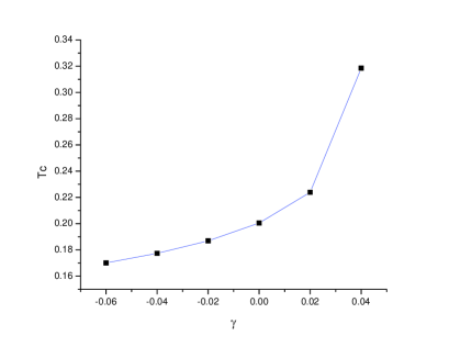
Figure 1: Graph shows the values of $T_{c}$ as a function of Weyl’s coupling . Here $\rho=1$.

FIG.1 shows that by increasing Weyl coupling $\gamma$, the critical temperature increases so condensation becomes more hard. Increasing scheme is a monotonic function of coupling $\gamma$.

III Existence of a Superconductor phase

Before we explained how the superconducting phase happens when the system undergoes a lower temperature than $T_{c}$. In this section we try to explain superconducting phase using matching technique. We like to mention here that we have followed largely the exposition given in GB1 .

We start by studying the system of equations of motion given in (22) and (23). The first observation is that the system (22) and (23) has the following non trivial solution in normal phase, i.e. when $T<T_{c}$ and $\psi=0$:

$$\phi=\phi_{0}(r) = \frac{\rho}{r_{+}^{2}}\left(1-\frac{r_{+}^{2}}{r^{2}}\right),\ \ \rho=\mu r_{+}^{2},$$ (26)

$$\psi \equiv 0.$$ (27)

One can verify this solution by examining the field equations in normal phase of $\psi=0$. The physical meaning of these solutions is the existence of the normal phase in which no condensation happens. We will now prove that there is a specific critical temperature $T_{c}$ that system under it goes to superconducting phase. It is useful to rewrite the (22) as:

$$\frac{d}{dr}\Big{[}(-r^{3}+24\gamma\frac{r_{+}^{4}}{r})\phi^{\prime}\Big{]}+(1+8\gamma\frac{r_{+}^{4}}{r^{4}})\frac{\psi^{2}\phi}{rr_{+}^{2}f}=0.$$ (28)

In the normal phase $T>T_{c}$ when $\psi=0$, the zero-order solution satisfies

$$\frac{d}{dr}\Big{[}(-r^{3}+24\gamma\frac{r_{+}^{4}}{r})\phi_{0}^{\prime}\Big{]}=0.$$ (29)

As a usual method for study instabilities of the models, we perturb $\phi(r)=\phi_{0}(r)+\delta\phi$. Then (28) up to the first-order perturbations shows:

$$\frac{d}{dr}\Big{[}(-r^{3}+24\gamma\frac{r_{+}^{4}}{r})\delta\phi^{\prime}\Big{]}\geq 0,$$ (30)

In the AdS boundary when the fields tend to their values on boundary surface,

$$(-r^{3}+24\gamma\frac{r_{+}^{4}}{r})\phi^{\prime}\to-r^{3}\phi^{\prime}\to-2\rho=-r^{3}\phi_{0}^{\prime},$$ (31)

consequently,

$$(-r^{3}+24\gamma\frac{r_{+}^{4}}{r})\delta\phi^{\prime}\to 0.$$ (32)

At AdS boundary,with aim of $\delta\phi|_{r_{+}}=0\Longrightarrow\delta\phi^{\prime}\leq 0$. So

$$\phi(r)\leq\phi_{0}(r).\$$ (33)

Now we consider second component of the gauge field, and we write it in the self-adjoint form:

$$\frac{d}{dr}\Big{[}(-r^{3}+24\gamma\frac{r_{+}^{4}}{r})\psi^{\prime}\Big{]}-(1+8\gamma\frac{r_{+}^{4}}{r^{4}})\frac{\psi^{2}\phi}{rr_{+}^{2}f^{2}}=0.$$ (34)

We define a new variable $X=r\psi$. Now, the boundary condition $\psi^{\prime}(r_{+})=0$ at the horizon implies that the new field satisfies $X^{\prime}_{+}=X_{+}/r_{+}$. Further in the asymptotic limit, $rfX^{\prime}\to 0$, so the existence of a condensatation state needs a typical critical point in field function$X$,

$$X^{\prime}(r_{{}_{T}})=0\wedge X^{\prime\prime}<0\wedge X>0.$$ (35)

Using $\phi_{0}(r)$ we have qualitatively verified that p-wave Weyl superconductors exist.

IV Critical temperature and condensation values by matching method

Because we showed that before, if we start from a scalar field model in the bulk, the on-shell stringy action, evaluated by the solutions of this scalar field has a kernel(Green function) which is exactly the same as the two point function of a relevant operator namely as ${\cal O}$ in the dual CFT.

Thus, we are ready to compute analytically the condensate $\langle{\cal O}\rangle$ with fixed $\rho$. We start by studying the boundary conditions in $z$ coordinate. Regularity at $z=1$, requires

$$\phi(1)=0\,,\hskip 28.45274pt\psi^{\prime}(1)=0\,,$$ (36)

The matching method starts by writing the series solution of the fields around the boundary points $z=1$ and $z=0$. We assume that these fields are non singular. So, the usual power series work for us. The next step is to match these two families smoothly. It means we suppose that here, fields and their first derivatives remain continuous. We have no logical reasons to have a jump in these boundary quantities.

IV.1 Solution near the horizon

We expand gauge fields $\{\phi,\psi\}$ near $z=1$ as

$$\phi(z) = \phi(1)-\phi^{\prime}(1)(1-z)+\frac{1}{2}\phi^{\prime\prime}(1)(1-z)^{2}+\cdots,$$ (37)

$$\psi(z) = \psi(1)-\psi^{\prime}(1)(1-z)+\frac{1}{2}\psi^{\prime\prime}(1)(1-z)^{2}+\cdots.$$ (38)

We set $a=-\phi^{\prime}(1)<0$ and $b=\psi(1)>0$ . For the 2^nd order coefficient $\phi$ we have (24):

$$\phi^{\prime\prime}(1) = -a\frac{1+72\gamma}{1-24\gamma}+\frac{1+8\gamma}{1-24\gamma}\frac{ab^{2}}{4r_{+}^{2}}.$$ (39)

So (37) reads as

$$\phi(z)=a\Big{[}(1-z)-\frac{(1-z)^{2}}{2(1-24\gamma)}\Big{(}1+72\gamma-\frac{b^{2}}{4r_{+}^{2}}(1+8\gamma)\Big{)}\Big{]}.$$ (40)

For $\psi$ similarly , via (25) as

$$\psi^{\prime\prime}(1) = -\frac{1}{32r_{+}^{2}}\Big{(}\frac{1+8\gamma}{1-8\gamma}\Big{)}a^{2}b.$$ (41)

So, we write the following series solution for scalar field (38)

$$\psi(z) = b\Big{[}1-\Big{(}\frac{1+8\gamma}{1-8\gamma}\Big{)}\frac{(1-z)^{2}}{64r_{+}^{2}}a^{2}\Big{]}.$$ (42)

IV.2 Solution near the asymptotic AdS region

From (24) and (25), in the asymptotic region we have

$$\phi(z) = \mu-\frac{\rho}{r_{+}^{2}}z^{2},$$ (43)

$$\psi(z) = \frac{<\cal O_{+}>}{r_{+}^{\Delta}}z^{\Delta}.$$ (44)

For renormalizability,we set $<\mathcal{O}_{-}>=0$. We clarify this quantization scheme as the following. A simple check shows that under mass bound, only $\Delta_{+}$ has an enough rapid fall off and the scalar field behaves as

$$\psi(r)\rightarrow r^{-(\Delta_{+}+2)}+r^{-\Delta_{+}}<\cal O_{+}>\,.$$ (45)

It means that the scalar field is dual to a quantum operator on the boundary with conformal dimension $\Delta_{+}$ and we can ignore $\cal O_{-}$. This is not the unique possible choice. It is easy to find that if mass be out of the BF bound, both of the terms with conformal dimensions $\Delta_{\pm}$ fall off and we can keep them. In conclusion, the quantization scheme is a valid procedure. In any case, the scalar field is asymptotic to $<\cal{O_{\pm}}>$ and these are dual to operators with dimension $\Delta_{\pm}$. However, in this work we limit ourselves to the fall off with $\Delta_{+}$.

IV.3 Matching and phase transition

Now, we smoothly join the solutions (40) and (42) with (43) and (44) respectively at $z=z_{m}$. Smoothly continuty requires

$$\phi^{z=0}|_{z_{m}}=\phi^{z=1}|_{z_{m}},\ \ \phi^{\prime z=0}|_{z_{m}}=\phi^{\prime z=1}|_{z_{m}}$$ (46)

$$\psi^{z=0}|_{z_{m}}=\psi^{z=1}|_{z_{m}},\ \ \psi^{\prime z=0}|_{z_{m}}=\psi^{\prime z=1}|_{z_{m}}$$ (47)

So, explicitly we obtain:

$$\mu-{\frac{\rho\,{z_{{m}}}^{2}}{{\pi}^{2}{T}^{2}}}=a\left(1-z_{{m}}-\frac{1}{2}\,{\frac{\left(1-z_{{m}}\right)^{2}\left(1+72\,\gamma-\frac{1}{4r_{+}^{2}}\,{b}^{2}\left(1+8\,\gamma\right)\right)}{1-24\,\gamma}}\right),$$ (48)

$$-\,{\frac{2\rho\,z_{{m}}}{{\pi}^{2}{T}^{2}}}=a\left(-1+{\frac{\left(1-z_{{m}}\right)\left(1+72\,\gamma-\frac{1}{4r_{+}^{2}}\,{b}^{2}\left(1+8\,\gamma\right)\right)}{1-24\,\gamma}}\right),$$ (49)

$$\frac{{z_{{m}}}^{\Delta}<\cal O_{+}>}{(\pi T)^{\Delta}}=b\left(1-{\frac{1}{64r_{+}^{2}}}\,{\frac{\left(1+8\,\gamma\right){a}^{2}\left(1-z_{{m}}\right)^{2}}{1-8\,\gamma}}\right),$$ (50)

$$\,{\frac{\Delta z_{m}^{\Delta-1}<\cal O_{+}>}{(\pi T)^{\Delta}}}=\frac{1}{32r_{+}^{2}}\,{\frac{b\left(1+8\,\gamma\right){a}^{2}\left(1-z_{{m}}\right)}{1-8\,\gamma}}.$$ (51)

Recalling that $r_{+}=\pi T$, after eliminating $ab^{2}$ from (48) and (49) gives

$$\mu = \frac{1}{2}\,{\frac{2\,\rho\,z_{{m}}-az_{{m}}{\pi}^{2}{T}^{2}+a{\pi}^{2}{T}^{2}}{{\pi}^{2}{T}^{2}}},$$ (52)

$$b = \sqrt{-{\frac{-8\,\rho\,z_{{m}}+192\,\rho\,z_{{m}}\gamma-384\,a\gamma\,{\pi}^{2}{T}^{2}+4\,az_{{m}}{\pi}^{2}{T}^{2}+288\,az_{{m}}\gamma\,{\pi}^{2}{T}^{2}}{a(1+8\,\gamma-z_{{m}}-8\,z_{{m}}\gamma)}}}.$$ (53)

We eliminate the $a^{2}b$ term from (50) and (51) and obtain

$$<\cal O_{+}> = \frac{\left(\pi\,T\right)^{\Delta}b}{{z_{{m}}}^{\Delta-1}\left(\frac{1}{2}\,\Delta+z_{{m}}\left(1-\frac{1}{2}\,\Delta\right)\right)}\ .$$ (54)

For non-vanishing b, we can eliminate $<\cal O_{+}>$ from (50) , (51) to obtain

$$a = 8\pi T{\frac{\,\sqrt{\left(1-z_{{m}}\right)\left(-\Delta-2\,z_{{m}}+z_{{m}}\Delta\right)\left(1+8\,\gamma\right)\Delta\,\left(-1+8\,\gamma\right)}}{\left(z_{{m}}-1\right)\left(-\Delta-2\,z_{{m}}+z_{{m}}\Delta\right)\left(1+8\,\gamma\right)}}.$$ (55)

With this $a$, from (53) we obtain

$$b = \sqrt{36\left(\left(\gamma+{\frac{1}{72}}\right)z_{{m}}-\frac{4}{3}\,\gamma\right){\pi}^{3}\sqrt{(1-z_{{m}})\left(-\Delta-2\,z_{{m}}+z_{{m}}\Delta\right)\left(1+8\,\gamma\right)\Delta\,\left(-1+8\,\gamma\right)}}$$ (56)

$$\times\sqrt{{\frac{{T}^{3}-T_{c}^{3}}{\left(\frac{1}{8}+\gamma\right)\left(-1+z_{{m}}\right)T\sqrt{\left(1-z_{{m}}\right)\left(1+8\,\gamma\right)\left(-1+8\,\gamma\right)\Delta\,\left(-2\,z_{{m}}+\Delta\,z_{{m}}-\Delta\right)}\pi}}}.$$

$T_{c}$ is defined as

$$T_{c} = \alpha(\gamma|z_{m}|\Delta)\rho^{\frac{1}{3}}$$ (57)

With

$$\alpha(\gamma|z_{m}|\Delta) = \frac{1}{2}\,\sqrt[3]{2(1+8\,\gamma)(-1+24\,\gamma)}\times\sqrt[3]{\frac{z_{m}}{z_{m}(1+72\gamma)-96\gamma}\sqrt{\frac{(1-z_{m})(-\Delta+z_{m}(\Delta-2))}{\Delta}}}$$ (58)

Here, as we know $-\frac{1}{16}<\gamma<\frac{1}{24}$. For positivity of the $T_{c}$, we have two possibilities (remembering that here the conformal dimension can be negative )

• Case $A:\ -\frac{1}{16}<\gamma<-\frac{1}{8},\gamma>\frac{z_{m}}{96-72z_{m}}$,

• Case $B:\ -\frac{1}{8}<\gamma<\frac{1}{24},\gamma<\frac{z_{m}}{96-72z_{m}}$.

In both cases, the conformal dimension reads as $\Delta>-\frac{2z_{m}}{1-z_{m}}$.

Figure 2: (Left)Numerical result shows the condensation $<{\cal O_{+}}>=<J_{x}^{1}>$ as a function of temperature. (Middle) Analytical result shows the $\frac{T_{c}}{\rho^{\frac{1}{3}}}$ as a function of the Weyl’s coupling for $z_{m}=\frac{1}{2}$,$\Delta=3$.. (Right) 3D plot of the normalized $T_{c}\equiv\frac{T_{c}}{\rho^{\frac{1}{3}}}$ as a function of the $\gamma,\Delta$ for $z_{m}=\frac{1}{2}$.

Finally $\langle{\cal O}_{+}\rangle$ is:

$$\langle{\cal O}_{+}\rangle=\beta(\gamma|z_{m}|\Delta)T_{c}^{\frac{3}{2}}T^{\Delta-\frac{1}{2}}\sqrt{1-(\frac{T}{T_{c}})^{3}},$$ (59)

where

$$\beta(\gamma|z_{m}|\Delta) = \frac{\sqrt{36\left(\left(\gamma+{\frac{1}{72}}\right)z_{{m}}-\frac{4}{3}\,\gamma\right){\pi}^{3}\sqrt{(1-z_{{m}})(-\Delta-2\,z_{{m}}+z_{{m}}\Delta)(1+8\,\gamma)\Delta\,(-1+8\,\gamma)}}}{{z_{{m}}}^{\Delta-1}(\frac{1}{2}\,\Delta+z_{{m}}(1-\frac{1}{2}\,\Delta))}$$ (60)

$$\times\frac{\pi^{\Delta}}{\sqrt{\left(\frac{1}{8}+\gamma\right)\left(1-z_{{m}}\right)\sqrt{\left(1-z_{{m}}\right)\left(1+8\,\gamma\right)\left(-1+8\,\gamma\right)\Delta\,\left(-2\,z_{{m}}+\Delta\,z_{{m}}-\Delta\right)}\pi}}.$$

We deduce that $\langle{\cal O}_{+}\rangle$ vanishes at $T=T_{c}$,and superconducting phase locates $T<T_{c}$. The mean field theory result $\langle{\cal O}_{+}\rangle\propto(1-T/T_{c})^{1/2}$ revisited. The value of $T_{c}$ via (57) is evaluated as $T_{c}\propto\sqrt[3]{\rho}$ is comparable with epl2 .

V Conclusions

In the present paper, we completed our former studies about the properties of Weyl’s corrected p-wave holographic superconductors in 5-dimensional $AdS$-Schwarzschild background. Firstly, we briefly clarified the key notes of gauge/gravity and how we relate the solutions of gravity to a quantity in field theory. The equations of motion in our interesting problem are nonlinear and coupled differential equations, so one cannot obtain analytic solutions to these equations in the closed form. Here we use the matching method. In this method, we match the asymptotic AdS solutions to the horizon solutions at a mid point, and then we find the expectation value of the dual operator $\langle{\cal O}_{+}\rangle$ and the critical temperature $T_{c}$ analytically. Surprisingly inspired from the string theory, the critical exponent of the condensation is independence from the Weyl correcxtions. These analytical results coincides completely on the previously numerical data epl2 .

References

• (1) J. M. Maldacena, Adv. Theor. Math. Phys. 2, 231 (1998).
• (2) C. P. Herzog, J. Phys. A 42 ,343001(2009) .
• (3) S. A. Hartnoll, Class. Quant. Grav. 26, 224002 (2009).
• (4) G. Policastro, D. T. Son, A. O. Starinets, Phys. Rev. Lett. 87, 081601 (2001).
• (5) P. Kovtun, D. T. Son, A. O. Starinets, JHEP10, 064 (2003).
• (6) S. A. Hartnoll, C. P. Herzog, G. T. Horowitz, JHEP 12 ,015 (2008).
• (7) G. T. Horowitz , M. M. Roberts, Phys. Rev. D 78, 126008 (2008).
• (8) R. Gregory, S. Kanno , J. Soda, JHEP10 ,010(2009) .
• (9) Y. Brihaye , B. Hartmann, Phys. Rev. D 81, 126008 (2010).
• (10) R.-G. Cai, Z.-Y. Nie,. H.-Q. Zhang, Phys. Rev. D 82, 066007 (2010).
• (11) Q. Pan , B. Wang, Phys. Lett. B. 693 (2010) 159.
• (12) Q. Pan, J. Jing, B. Wang, JHEP 11 ,088 (2011).
• (13) R.-G. Cai , H.-Q. Zhang, Phys. Rev. D81, 066003(2010).
• (14) D. Momeni, M. R. Setare, N. Majd, JHEP 1105 ,118(2011),arXiv:1003.0376 [hep-th].
• (15) E. Nakano, W.-Y. Wen, Phys.Rev.D78,046004(2008).
• (16) D. Momeni, E. Nakano, M. R. Setare and W. -Y. Wen, Int. J. Mod. Phys. A 28 (2013) 1350024 [arXiv:1108.4340 [hep-th]].
• (17) M. R. Setare, D. Momeni, EPL, 96, 60006(2011) ,arXiv:1106.1025.
• (18) Y. Liu, Y. Peng, B. Wang, arXiv:1202.3586 [hep-th].
• (19) Q. Pan, J. Jing, B. Wang, Phys. Rev. D 84, 126020 (2011).
• (20) G. Tallarita, S. Thomas, JHEP 1012:090 (2010).
• (21) Q. Pan, J. Jing , B. Wang Phys.Rev. D84, 126020 (2011) .
• (22) D. Momeni, M. Raza, R. Myrzakulov, arXiv: 1305.3541, Journal of Gravity 2013 (2013)782512.
• (23) Y.-Q. Wang, Y.-X. Liu, R.-G. Cai, S. Takeuchi, H.-Q. Zhang, arXiv:1205.4406 [hep-th].
• (24) S. S. Gubser, S. S. Pufu, JHEP 11, 033 (2008).
• (25) C. P. S. Herzog, S. Pufu, JHEP 0904 , 126 (2009).
• (26) M. Ammon ,J. Erdmenger ,V. Grass, P. Kerner ,A. O’Bannon, Phys. Lett. B 686 ,192(2010) .
• (27) D. Momeni, M. Raza, R. Myrzakulov, arXiv:1307.2497.
• (28) X.-H. Ge, S. F. Tu, B. Wang , arXiv:1209.4272.
• (29) D, Gao ,Phys. Lett. A 376 ,1705(2012),arXiv:1112.2422.
• (30) H.-B. Zeng, Z.-Y. Fan, H.-S. Zong, Phys.Rev.D82:126008,2010 , arXiv:1007.4151.
• (31) F. Benini, C. P. Herzog, A. Yarom, Phys.Lett.B701:626(2011),arXiv:1006.0731 .
• (32) J.-W. Chen, Y.-J. Kao, D. Maity, W.-Y. Wen, C.-P. Yeh, Phys. Rev. D81:106008 (2010), arXiv:1003.2991 .
• (33) C. P. Herzog, Phys. Rev.  D81, 126009 (2010).
• (34) S. Kanno, Class. Quant. Grav. 28, 127001(2011) .
• (35) H.-B. Zeng, X. Gao, Y. Jiang, H.-S. Zong, JHEP 05, 2 (2011).
• (36) Q. Pan, J. Jing , B. Wang , S. Chen ,JHEP, 1206, 087(2012).
• (37) D. Momeni , M. Raza ,M. R. Setare , R, Myrzakulov, Int. J. Theor. Phys,DOI 10.1007/s10773-013-1569-4.
• (38) D. Momeni, M.R. Setare, Mod. Phys. Lett. A, 26, 38,2889 (2011), arXiv:1106.0431 .
• (39) D. Momeni, M.R. Setare,Ratbay Myrzakulov, Int. J. Mod. Phys. A27, 1250128 (2012), arXiv:1209.3104.
• (40) J.-P. Wu, Y. Cao, X.-M. Kuang, W.-J. Li, Phys.Lett.B697:153 (2011).
• (41) M. R. Setare, D. Momeni, R. Myrzakulov, M. Raza, arXiv: 1210.1062.
• (42) D. Momeni,N. Majd, R. Myrzakulov, EPL, 97 ,61001(2012),arXiv: 1204.1246.
• (43) J.-P. Wu, arXiv:1006.0456 [hep-th].
• (44) D.-Z. Ma, Y. Cao, J.-P. Wu ,Phys. Lett. B 704, 604(2011) .
• (45) Z. Zhao, Q. Pan and J. Jing, Phys. Lett. B 719, 440 (2013) [arXiv:1212.3062 [hep-th]].
• (46) J.-P. Wu, Y. Cao, X.-M. Kuang, W.-J. Li, Phys. Lett. B697, 153 (2011).
• (47) R. Manvelyan, E. Radu, and D. H. Tchrakian, Phys. Lett. B 677, 79 (2009).
• (48) I. T. Drummond , S. J. Hathrell, Phys. Rev. D 22, 343 (1980).
• (49) R.-G. Cai, H.F. Li, H.Q. Zhang, Phys.Rev.D83:126007(2011).
• (50) A. Ritz and J. Ward, Phys. Rev. D 79 (2009) 066003.