A view from inside iron-based superconductors

Abstract

Muon spin spectroscopy is one of the most powerful tools to investigate the microscopic properties of superconductors. In this manuscript, an overview on some of the main achievements obtained by this technique in the iron-based superconductors (IBS) are presented. It is shown how the muons allow to probe the whole phase diagram of IBS, from the magnetic to the superconducting phase, and their sensitivity to unravel the modifications of the magnetic and the superconducting order parameters, as the phase diagram is spanned either by charge doping, by an external pressure or by introducing magnetic and non-magnetic impurities. Moreover, it is highlighted that the muons are unique probes for the study of the nanoscopic coexistence between magnetism and superconductivity taking place at the crossover between the two ground-states.

1 Introduction

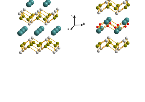
Figure 1: Crystalline structures of AFe₂As₂ (with A alkali ions) (left) and of LnFeAsO_1-xF_x (with Ln a lanthanide ion) (right) Fe-based superconductors. For the AFe₂As₂ superconductors the unit cell projected along the $c$ axis is also shown at the top left part of the figure.

More than $20$ years after the discovery of high-temperature superconductivity (HTSC) in the cuprates [1, 2], the observation of critical temperatures ($T_{c}$) approaching $55$ K in iron-based pnictides [3, 4] has renewed the interest for superconductivity and for the fascinating phenomenology it gives rise to [5]. Remarkably, the iron-based superconductors (IBS hereafter) share many similarities with the cuprates [6, 7, 8, 9, 10]. First of all, both families of materials are characterized by layered structures, involving FePn layers (with Pn = As, P or Se) in the IBS [11] and CuO₂ planes in the cuprates [12] (see Figs. 1 and 2 for the structure of these two classes of materials, respectively). The layered structure gives rise to a sizeable anisotropy in the transport and magnetic properties, which is more marked in the latter compounds. The high anisotropy is known to cause an enhancement of the flux lines lattice (FLL) mobility and to yield detrimental dissipative phenomena [15, 16] which could hinder the technological applicability of these materials. Still, the IBS are characterized by an anisotropy which is not so pronounced and, accordingly, by a lower FLL mobility.[17, 18, 19, 20, 21] At the same time they show upper critical fields often exceeding $60$ Tesla [22, 23], making the IBS rather promising for applications.

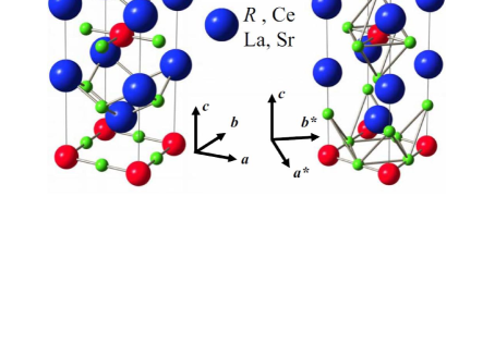
Figure 2: Crystalline structures of typical electron- (left) and hole-doped (right) cuprate materials (Figure reprinted from Ref.[13]. Copyright (2010) by the American Physical Society).

The high upper critical fields imply rather short coherence lengths, reaching few nanometers along the FeAs planes, so that these materials are weakly sensitive to disorder and, in particular, to non-magnetic impurities. Another relevant similarity between the IBS and the cuprates is that superconductivity is obtained by charge-doping a strongly correlated electron system with a magnetic ground-state in both families of compounds [2, 10, 24]. This is shown in the typical electronic phase diagrams reported in Figs. 3 and 4 for the IBS and for the cuprates, respectively.

The correlations are certainly more relevant in the cuprates where the significant Coulomb repulsion yields to an insulating ground-state, while in the IBS the magnetic precursors are metallic. In particular, a multi-band scenario applies to pnictides where the $5$ bands involving all the Fe $3d$ orbitals contribute to the density of states at the Fermi level [25, 26, 27]. Notice that a metallic behaviour with reconstruction of the Fermi surface (FS) is observed also in the cuprates after a few percent of charge doping, prior to the onset of the superconducting ground-state [28]. At the same time, in the pnictides the scenario of an antiferromagnetic (AFM) phase arising just from the FS nesting remains controversial, since non-negligible correlations, bringing those samples close to a Mott-like transition, should also be considered [29, 30, 31, 32, 33]. As a result, several authors have described the magnetism in pnictides in terms of effective Hamiltonians for localized magnetic moments in the presence of competing frustrating interactions [29, 30, 34, 35, 36].

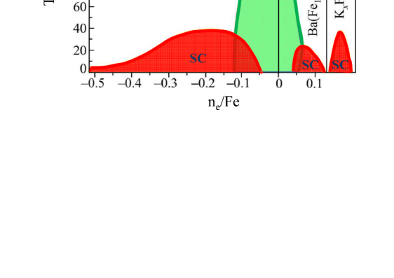
Figure 3: Typical electronic phase diagram for the $122$ family of pnictide materials as a function of the number of extra-electrons n_e per Fe atom, both in the case of hole- and electron-doping.

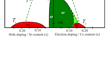
Figure 4: Typical electronic phase diagram for cuprate materials both in the case of hole- and electron-doping (Figure reprinted from Ref. [13]. Copyright (2010) by the American Physical Society).

The phase diagrams described above are obtained by doping the parent compound with charges (either holes or electrons). Several chemical substitutions have been investigated in order to achieve such goal. However, as far as the substitution of the Fe ions with other transition metal (TM) elements is considered, the effectiveness of charge doping is still under strong debate and has been subject of recent intense efforts both on the computational and on the experimental sides, particularly in the case of Co for Fe substitution. Contrasting results have been reported from density-functional theory (DFT) calculations [37, 38] as well as from measurements via x-rays absorption [39, 40] and photoemission [41] spectroscopies. At the same time, the role of isovalent substitutions such as Fe_1-xRu_x attracted great interest both in LnFeAsO_1-xF_x (the so-called $1111$ family of IBS, with Ln a lanthanide ion) and in the AFe₂As₂ (the $122$ IBS, with A an alkali ion) compounds. The Fe_1-xRu_x dilution does not induce a superconducting phase in LaFeAsO [36], at variance with what is observed in BaFe₂As₂ [42, 43]. Still, it induces a reentrant static magnetic phase nanoscopically coexisting with superconductivity in the optimally Fluorine-doped $1111$ IBS for different Ln ions [44, 45] (see Fig. 5).

It should be mentioned that, as an alternative to chemical doping of the parental compounds, the application of an external [46, 47, 48, 49] or of a chemical [50] pressure has been reported to be a useful tool to span through the different electronic ground states of these materials. However, the effects of chemical doping and pressures are not equivalent at all. In particular, the increase of pressure is known to involve also the modification of more subtle many-body effects like the Kondo screening in the presence of conduction carriers hybridized with unpaired $f$ electrons [51]. It has been established theoretically that the Kondo effect and superconductivity strongly compete in $1111$ pnictide compounds [52]. For instance, this is clearly the case for Ce-based $1111$ compounds where superconductivity is induced by charge doping [53, 54, 55] but bulk superconductivity cannot be induced neither by external [56] nor by chemical [57] pressures, which are naively expected to enhance the Kondo coupling.

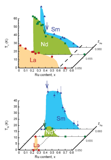
Figure 5: Electronic phase diagram for optimally Fluorine-doped LnFeAsO_1-yF_y $1111$ materials as a function of the amount of Fe_1-xRu_x dilution, with Ln= Sm, Nd, La [45].

The similarities among IBS and cuprates discussed above suggested that the understanding of the microscopic mechanisms at work in IBS would have eventually lead to the clarification of the long debated origin of HTSC. The interplay between magnetism and superconductivity have lead to the idea that in both classes of materials a pairing involving the spin excitations could be present [8, 58]. However, in spite of the huge efforts both on the experimental and theoretical sides, currently it is not yet clear whether such a pairing mechanism is indeed driving HTSC. On the other hand, it is well established that for the hole-doped cuprates the symmetry of the order parameter is d-wave [59], while it is s-wave for the electron-doped cuprates [60]. In the IBS, the symmetry of the order parameter is presently subject of an intense debate. While it was initially suggested that the FS nesting would favour a magnetic coupling between hole-like and electron-like bands, yielding to an $s_{\pm}$ symmetry of the order parameter [61, 62], more recent studies suggested that a conventional $s$ wave symmetry would be more likely, with a pairing mediated by orbital current fluctuations [63, 64]. Even if the nature of the pairing mechanism is still undisclosed, it seems to be well established that a conventional phonon-mediated superconductivity is unlikely in IBS [65]. Overall, the IBS appear as rather complex systems, and more than $5$ years after their discovery their understanding still demands for a significant experimental investigation and a suitable theoretical modelling.

Muon spin spectroscopy ($\mu^{+}$SR) has played a major role in the clarification of the electronic and magnetic properties of cuprate materials first [66, 67] and of the IBS more recently. The muons act as nanoscopic Hall sensors which allow to map the local fields inside those materials and to track their time evolution. In fact, they allow to probe the spin dynamics, the local field arising from the onset of a magnetic order or the field distribution generated by the flux lines in the mixed state [67, 68, 69, 70, 71, 72]. The local nature of the technique is particularly useful to evidence the intrinsic microscopic electronic inhomogeneities leading to the nanoscopic coexistence of magnetic and superconducting domains and/or of charge poor and charge rich regions, which characterize both the IBS [44, 73] and the cuprates [82, 83]. In this respect, $\mu^{+}$SR is rather a unique tool, complementary to non-local techniques as neutron scattering or to other local techniques as NMR, which can suffer from RF penetration and/or excessive line broadening problems. In the following, we present some of the main achievements obtained by means of $\mu^{+}$SR in the IBS. First, it is shown how the muons allow to investigate the whole phase diagram of these materials, from the magnetic to the superconducting phase, as well as the nature of the phase transition between the superconducting and magnetic ground-states. It is then shown how the study of the transverse field relaxation in the superconducting state provides useful information on the evolution of the superconducting transition temperature with the concentration of Cooper pairs. We shall mostly concentrate on the static properties of IBS by referring to the 1111 family and on the effect of heterovalent and isovalent chemical substitutions on its phase diagram and on the superconducting properties. The scenario observed for the 122 family of IBS will also be briefly recalled, while for the $\mu$SR studies carried out in other families of IBS, as the 11 chalcogenides and the 111 the reader can refer to Refs. [74, 75, 76, 77, 78, 79, 80] and Ref. [81], respectively.

2 The zero field muon spin polarization in the magnetic phase

The full spin-polarization of the positive muon ($\mu^{+}$) beams produced at meson factories, such as ISIS (Rutherford-Appleton Laboratories, UK) and S$\mu$S (Paul Scherrer Institut, PSI, Switzerland), is the prerequisite for running $\mu^{+}$SR experiments. The possibility to work with fully polarized beams has the great advantage, in comparison to other local-probe techniques such as NMR, that there is no need to perturb the system under investigation with an external polarizing magnetic field. Accordingly, local magnetism can be investigated even in conditions of zero-magnetic field (ZF).

In general, at a given temperature ($T$), the ZF $\mu^{+}$ depolarization as a function of the time ($t$) elapsed after the implantation into the sample is described by

$$\frac{A_{ZF}(t)}{A_{0}}=\left(1-a_{s}\right)G_{KT}^{H}(t)+a_{s}G_{ZF}^{s}(t)\,\,\,.$$ (1)

Here $A_{0}$ is an instrument-dependent constant corresponding to the condition of full spin-polarization extrapolated at $t\rightarrow 0$, $a_{s}$ represents the fraction of $\mu^{+}$ implanted into the investigated sample while $\left(1-a_{s}\right)$ is the background fraction. This latter quantity includes, for example, the $\mu^{+}$ implanted into the sample holder or into the cryostat walls and probing weakly-magnetic regions whose main contribution comes from magnetism of nuclear origin. This typically results in a Gaussian Kubo-Toyabe depolarization function $G_{KT}^{H}(t)$, which at early times shows a Gaussian trend $G_{KT}^{H}(t)\sim e^{-\frac{\left(\sigma_{N}\right)^{2}t^{2}}{2}}$, governed by a weakly $T$-dependent factor $\sigma_{N}$. Both MuSR and EMU, at ISIS, and GPS and Dolly, at PSI, are designed as low-background spectrometers, namely allowing one to achieve the condition $a_{s}\simeq 1$. However, the background term in Eq. 1 is of crucial importance while analyzing data from measurements under applied pressure performed, for instance, at the GPD facility of S$\mu$S [48, 84, 85]. Here, the thick walls of the pressure cell are able to stop a sizeable fraction of $\mu^{+}$ leading typically to $a_{s}\simeq\left(1-a_{s}\right)\simeq 0.5$. Nevertheless, since all the measurements to be discussed subsequently have been performed in the low-background spectrometers, from now on it is assumed that $a_{s}=1$, so that $A_{ZF}(t)/A_{0}=G^{s}_{ZF}(t)$, with $G_{ZF}^{s}(t)$ the spin-depolarization function of the $\mu^{+}$ implanted into the sample. As it will be explained in the following, in the IBS the ZF depolarization can be described rather well by

$$\frac{A_{ZF}(t)}{A_{0}}=G_{ZF}^{s}(t) = \left[1-V_{m}(T)\right]G_{KT}^{s}(t){}$$ (2)

$$+ \sum_{i=1}^{N}\zeta_{i}\left[a_{i}^{Tr}(T)F_{i}(t)D_{i}^{Tr}(t)+a_{i}^{L}(T)D_{i}^{L}(t)\right]\,\,\,.$$

where $G_{KT}^{s}(t)\simeq e^{-\frac{\left(\sigma_{N}^{s}\right)^{2}t^{2}}{2}}$ for $\sigma_{N}^{s}t\ll 1$, is the Kubo-Toyabe function describing the relaxation arising from the dipolar coupling with the nuclei in the sample. Eq. 2 typically holds in the case of materials undergoing a phase transition to a magnetically-ordered state at a temperature $T_{N}$. Accordingly, a set of ZF-$\mu^{+}$SR measurements at different $T$ values allows one to access several microscopic quantities associated both with the ordered and with the paramagnetic phases. The parameter $V_{m}(T)$ represents the fraction of $\mu^{+}$ implanted into the sample and feeling a spontaneous static magnetic field, namely the sample magnetic volume fraction, from which one can estimate $T_{N}$. The ideal case of a step-like behaviour of $V_{m}(T)$ at $T_{N}$ is modified in real systems where a spatial distribution of $T_{N}(\bm{r})$ can be present. The assumption of a Gaussian-like distribution of local transition temperatures generally leads to the following phenomenological expression for $V_{m}(T)$

$$V_{m}(T)=\frac{1}{2}\;\textrm{erfc}\left[\frac{T-T_{N}}{\sqrt{2}\Delta}\right]$$ (3)

where $\textrm{erfc}(x)$ is the complementary error function. A fitting procedure to the experimental $V_{m}(T)$ data according to Eq. 3 allows a precise definition both of $T_{N}$ and of the relative width $\Delta$ of the transition itself. In particular, the $T_{N}$ value extracted from Eq. 3 is an average value defined as the $T$ value corresponding to $50$ % of the magnetic volume fraction.

Let us now consider the behaviour of the depolarization function at $T\ll T_{N}$. In general, one should account for the possibility of different phases in the sample volume, i. e. for a macroscopic or nanoscopic (see Sect. 3) segregation of magnetic and paramagnetic phases leading to the condition $V_{m}(T)<1$. Here, it is assumed $V_{m}(T)=1$ in the simplified assumption of a homogeneous fully-magnetic sample. Then the first term in Eq. 2 drops out, leading to

$$\frac{A_{ZF}(t)}{A_{0}}=\sum_{i=1}^{N}\zeta_{i}\left[a_{i}^{Tr}(T)F_{i}(t)D_{i}^{Tr}(t)+a_{i}^{L}(T)D_{i}^{L}(t)\right].$$ (4)

The presence of $N$ crystallographically-inequivalent stopping sites for $\mu^{+}$ is accounted for by the sum over the index $i$. Each stopping site is characterized by its corresponding stopping probability $\zeta_{i}$, with $\sum_{i}\zeta_{i}=1$. Accordingly, the quantities $\zeta_{i}a_{i}^{Tr}(T)$ and $\zeta_{i}a_{i}^{L}(T)$ represent the fractions of all the implanted $\mu^{+}$ at the site $i$ that feel a static field in transversal ($Tr$) and longitudinal ($L$) directions with respect to the initial $\mu^{+}$ polarization, respectively. Thus, the following relation holds under general assumptions

$$\sum_{i=1}^{N}\zeta_{i}\left[a_{i}^{Tr}(T)+a_{i}^{L}(T)\right]=V_{m}(T).$$ (5)

For powder samples, in the ideal condition that long-range magnetic order develops throughout the whole sample volume, the relations

$$\sum_{i=1}^{N}\zeta_{i}a_{i}^{Tr}(T\ll T_{N})=\frac{2}{3}\qquad\textrm{and}\qquad\sum_{i=1}^{N}\zeta_{i}a_{i}^{L}(T\ll T_{N})=\frac{1}{3}$$ (6)

follow from straightforward geometrical arguments. This is commonly addressed to as the $2/3$ - $1/3$ rule. The function $F_{i}(t)$ in Eq. 4 describes the coherent oscillations associated with the Larmor precession of the $Tr$ fraction of muon spins around the local magnetic field $B_{\mu}$, generated by the long-range magnetic order. The distribution in the magnitude of the local fields give rise to the corresponding damping functions $D_{i}^{Tr}(t)$. On the other hand, $\mu^{+}$ belonging to the $L$ fraction do not precess and usually probe longitudinal $T_{1}$-like dynamical processes resulting in a relaxing tail described by $D_{i}^{L}(t)$. Due to the limited time window, to the finite number of counts and to the comparable values of the relaxation constants, it is often difficult to distinguish the longitudinal relaxations of different $\mu^{+}$ sites, which eventually merge in a common $D^{L}(t)$. Typically, $D^{L}(t)$ is an exponentially-relaxing component characterized by weak relaxation rates, typically of the order of $0.1\;\mu$s^-1.

In the opposite temperature limit ($T\gg T_{N}$), namely in the paramagnetic phase, no static fields of electronic origin alter the initial $\mu^{+}$ polarization. In this case, $V_{m}(T)=\sum_{i}\zeta_{i}a_{i}^{Tr}=\sum_{i}\zeta_{i}a_{i}^{L}=0$ and the whole second term in Eq. 2 vanishes, leading to

$$A_{ZF}(t)\simeq A_{0}e^{-\frac{\left(\sigma_{N}^{s}\right)^{2}t^{2}}{2}}\,\,\,,$$ (7)

namely the decay is determined by the dipolar field distribution arising from the nuclear magnetic moments.

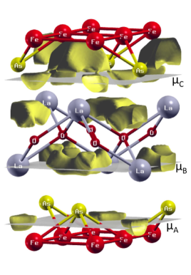
Figure 6: Electrostatic landscape for LaFeAsO after DFT calculations [84]. Iso-potential curves corresponding to the thermalization positions for $\mu^{+}$ are represented as yellow shaded regions. Only sites “A” and “B” are stable minima while site “C” is unstable against the zero-point energy of $\mu^{+}$.

In the case of $1111$ Fe-based oxy-pnictide materials, the crystallographic sites for the thermalization of $\mu^{+}$ have been computed by means of DFT calculations of the electrostatic potential as reported, e. g., in [84, 86] (see also [85] for the case of RECoPO samples). The results of the calculations yield $N=2$ stable minima in addition to a further site which, however, is unstable against the zero-point motion of $\mu^{+}$. In particular, one site is close to the FeAs layers while the other one is much closer to the RE ions (see Fig. 6). These are referred to as “A” (or “1”) and “B” (or “2”) in the following, respectively, while the unstable one is referred to as “C”. For the sake of clarity, the electrostatic landscape for LaFeAsO is reported in Fig. 6 together with the crystallographic positions of both stable and unstable sites. As a first-order approximation, both $\zeta_{1}$ and $\zeta_{2}$ are $T$-independent quantities. This is quite reasonable since the diffusion of $\mu^{+}$ is typically a marginal process in the explored $T$-range ($T\lesssim 170$ K). In the case of REFeAsO materials, one typically finds $\zeta_{1}/\zeta_{2}\simeq 4$ for the occupation probabilities of the sites $\zeta_{i}$, independently from the actual chemical stoichiometry. The lineshapes associated with the two different $\mu^{+}$ sites in REFeAsO_1-xF_x (RE = Ce) are narrow enough to resolve signals from both of them in the undoped and in the slightly doped ($x=0.03$) materials only [53]. A further increase in $x$ yields a broadening of the frequency distribution, making the smaller signal from site “B” unobservable. The interpretation of the two contributions as signals coming from two inequivalent sites is strongly supported by the experimental findings for all the investigated samples. In particular, both signals show a fast growth either of the oscillation frequency or of the damping at the same critical temperature $T_{N}$, hence reflecting the same microscopic electronic environment.

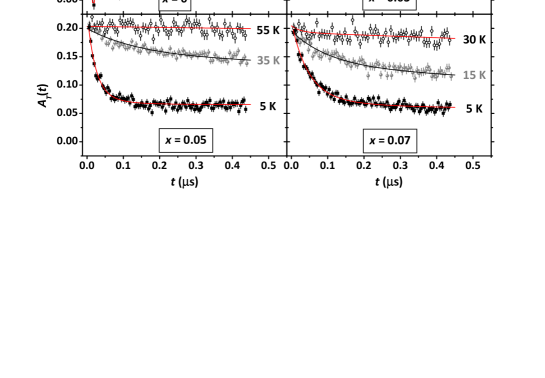
Figure 7: Experimental spin-depolarization at low-$T$ in ZF conditions for CeFe_1-xCo_xAsO in the low-$x$ region of the electronic phase diagram [55]. The strong increase of the transversal damping with increasing $x$ is the experimental trademark of the progressive disordering of the magnetic phase towards the limit of short-range magnetic order coexisting with superconductivity.

The $\mu^{+}$ implanted in both sites give rise to a characteristic beat in the $\mu^{+}$ depolarization function of the LaFeAsO parental magnetic compound at $T\ll T_{N}$ [87]. On the other hand, this is not the case in compounds based on magnetic rare-earth (RE) ions where only one oscillating signal is detected from site “1” (see Fig. 7). In fact, site “2” being very close to the large RE magnetic moments which generate a broad field distribution, shows an extremely fast signal decay [53]. Both in the case of LaFeAsO and CeFeAsO, the function $F_{1}(t)=\cos\left(\gamma_{\mu}B_{\mu_{1}}t\right)$ describes the data quite well ($\gamma_{\mu}=2\pi\times 1.355\times 10^{-2}$ MHz/G being the $\mu^{+}$gyromagnetic ratio). As reported in Fig. 8, also in the case of the parent compounds of the $122$ family (e.g. BaFe₂As₂) one clearly observes beats arising from the signals of two muon sites [88].

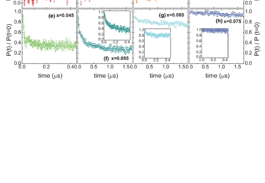
Figure 8: Experimental spin-depolarization at low-$T$ in ZF conditions for Ba(Fe_1-xCo_x)₂As₂ in the low-$x$ regime (Figure reprinted from Ref. [88]. Copyright (2012) by the American Physical Society).

When considering slightly charge-doped magnetic compounds, long-range magnetism is still probed by $\mu^{+}$ even if some qualitative changes in the spin-depolarization functions should be considered. First of all, the oscillating cosine-like function considered above in the case of the parent compounds should be modified to $F_{1}(t)=J_{0}\left(\gamma_{\mu}B_{\mu_{1}}t\right)$ ($J_{0}$ standing for a zeroth-order first-kind Bessel function). This function better describes the field distribution and the gradual modification of the spin density wave (SDW) phase commensurability upon increasing the charge doping [89, 90]. On the other hand, the increase in the degree of magnetic disorder yields to an enhancement of the transversal damping, with respect to what observed in the parental compounds. This is evident both in CeFeAsO_1-xF_x, CeFe_1-xCo_xAsO (see Fig. 7) and in Ba(Fe_1-xCo_x)₂As₂ (see Fig. 8).

By further increasing $x$, the disorder is so strong that the oscillations are completely overdamped, hence reflecting an extremely broad distribution of static magnetic fields at the $\mu^{+}$ site. Even in this highly disordered configuration, one can give an estimate of the typical internal field of the magnetic phase by referring to the width of the field distribution (i. e., the squared root of the second moment). It should be remarked that in the case of overdamped transversal oscillations one should carefully exclude dynamical effects on the muon depolarization function. In these cases, one useful way to distinguish among the two scenarios is to perform a longitudinal-field (LF) scan. Only in the case of a static distribution of local fields the application of a strong enough magnetic field allows one to quench the spin-depolarization and to estimate the width of the static distribution (see [53] for example).

In general, the three main microscopic contributions to the local field at the muon site $B_{\mu}$ come from the dipolar, the transferred hyperfine and the Lorentz terms (see [85] and references therein)

$$B_{\mu}=\left|\textbf{B}_{dip}(\mathbf{r}_{\mu})+\textbf{B}_{c}(\mathbf{r}_{\mu})+\textbf{B}_{L}\right|.$$ (8)

The commensurate SDW actually corresponds to an AFM configuration and $B_{\mu_{1}}(T)$ is proportional to the sublattice magnetization $M_{st}(T)$ (see [84]). Owing to the crystallographic symmetry of site “1”, for an AFM order the only relevant contribution is the dipolar term, since the hyperfine contribution is almost entirely averaged out and $\textbf{B}_{L}$ can be neglected because of the vanishing macroscopic magnetization. Accordingly, if the crystallographic position of site “1” is precisely known it is possible to estimate the Fe magnetic moment from dipolar sums. From the internal field at the $\mu^{+}$ site measured in the case of $1111$ materials with no charge doping, one derives $\mu_{Fe}\simeq 0.65\;\mu_{B}$ for the Fe magnetic moment [84]. Even in the case of a sizeable degrees of magnetic disorder, the order parameter can be estimated from the width of the distribution of static local magnetic fields, as explained above.

3 Electronic phase diagram and the coexistence between magnetism and superconductivity

The main typical outputs of ZF-$\mu^{+}$SR experiments on magnetic materials are the order parameter and the sample volume fraction $V_{m}$, which can be evaluated from Eq. 2 as two independent fitting parameters. The great advantage of $\mu$SR when compared, for example, to neutron scattering is that it is a local probe technique which can detect a static magnetic order even when the coherence length is reduced to a few lattice steps and the system is quite inhomogeneous. Thus, $\mu^{+}$SR is perfectly suited to investigate the details of the transition between the magnetic and the superconducting phases and it has been deeply employed in pnictide superconductors to study the phase diagram obtained upon tuning in a controlled way some key-parameter such as the level of iso- and/or hetero-valent chemical substitutions, the structural parameters and the external pressure.

The crossover region between the magnetic and superconducting electronic ground states is of crucial relevance for the understanding of the intrinsic microscopic properties of pnictide materials. According to some theoretical models [91, 92], the experimental finding of coexistence between magnetism and superconductivity over a certain region of the phase diagram is an indication of an unconventional pairing among the supercarriers. Still, one should clarify which is the spatial level of coexistence or, in other terms, the degree of spatial intertwining of the two different order parameters. This degree can be quantified by a characteristic length scale $d$ describing the typical distance among magnetic or, alternatively, among superconducting domains. The strength of the claim of “coexistence between magnetism and superconductivity” is crucially depending on the order of magnitude of $d$. In the case $d\sim 100$ nm $-1$ $\mu$m, one typically refers to the so-called macroscopic or mesoscopic segregation of the two ground states. No definitive conclusion can be obtained in this case concerning the symmetry of the superconducting order parameter since the ground states occupy different spatial regions that are in principle mutually independent from each other. This condition can be driven for instance by trivial inhomogeneity of the chemical doping in the investigated material and it has typically to deal with extrinsic properties. The opposite case $d\sim 1-10$ nm is by far more interesting since it implies a much finer intertwining of the two order parameters (nanoscopic segregation or nanoscopic coexistence) towards the limit of the so-called “atomic coexistence” ideally realized in the same spatial position. This is clearly a much more interesting limit in order to draw conclusions on the intrinsic properties of the examined materials.

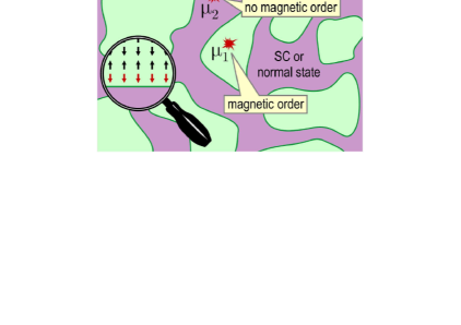
Figure 9: (Color online) Sketchy representation of the model of phase segregation of magnetism and superconductivity (Figure reprinted from Ref. [93]. Copyright (2009) by the American Physical Society). The nanoscopic coexistence is realized whether the order-of-magnitude of the mean distance among magnetic domains (green droplets) is close to $d\sim 1$ nm, namely the spatial range of the magnetic dipolar field generated by uncompensated Fe moments on the domain walls (red arrows).

The experimental way of treating this problem is typically not trivial at all and qualitatively different results can be obtained as a function both of the chemical homogeneity of the investigated sample and of the technique employed. In this respect, it should be stressed that $\mu^{+}$SR measurements are of crucial importance for the reasons outlined above. The local nature of the technique allows one to be sensitive to the disordered magnetism that is typically realized in the case of nanoscopic coexistence. As a further advantage with respect to other local techniques like, e. g. NMR, only $\mu^{+}$SR allows to precisely estimate $V_{m}$. This information is of major importance in order to quantify the order of magnitude of $d$. Let’s refer to Fig. 9 where a sketchy representation of the phase segregation of two different order parameters is reported [93]. The global magnetic moment within the domains is null due to the AFM correlations characteristic of the SDW phase. Still, $\mu^{+}$ are able to feel the dipolar field generated by the uncompensated magnetic moments on the domain walls (see red arrows in the figure under the magnifying lens). In the case of the dipolar field generated by Fe in the case of $1111$ oxy-pnictide materials, one can roughly deduce that the minimal distance required in order to probe magnetism under these conditions for $\mu^{+}$ implanted out of the domains is of the order of $1$ nm [94]. In the case of the mesoscopic segregation of the order parameters, $\mu^{+}$ implanted out of the magnetic domains (and conventionally labelled as $\mu_{2}^{+}$) are on the average too far away from the domains themselves to probe static magnetism and only $\mu^{+}$ implanted into the domains (and conventionally labelled as $\mu_{1}^{+}$) give rise to a magnetic signal. As a result, $V_{m}<1$ in the case of mesoscopic segregation and a value $\left(1-V_{m}\right)>0$ is measured as a paramagnetic volume fraction, accordingly. This behaviour was clearly enlightened in the case of La-based $1111$ samples with the phase diagram being swept both by the increasing concentration of electrons triggered by the O_1-xF_x substitution [95] or by the application of external hydrostatic pressure [48], at variance with what is typically reported for $1111$ materials based on magnetic RE ions, as it will be shown subsequently.

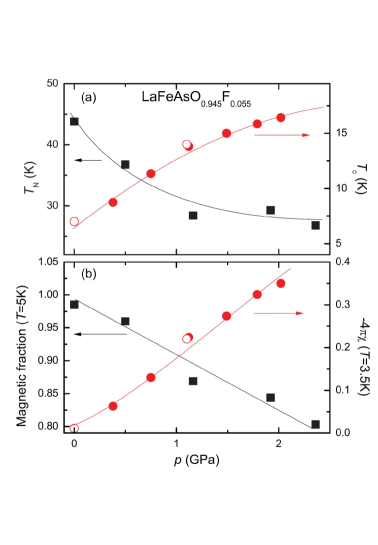
Figure 10: Effect of pressure ($P$) on magnetism and superconductivity in LaFeAsO_0.945F_0.055 [48]. Upper panel: $P$-dependence of the magnetic and superconducting critical temperatures. Lower panel: $P$-dependence of the magnetic and superconducting volume fractions.

At the same time, early reports on hole-doped $122$ compounds like Ba_1-xK_xFe₂As₂ seemed to confirm the picture of the mesoscopic segregation [93] at variance with what reported about electron-doped compounds like Ba(Fe_1-xCo_x)₂As₂ [88, 96, 97]. It should be remarked that independent quantifications of the superconducting shielding fractions of samples displaying mesoscopic segregation (e.g. derived from dc magnetometry or ac susceptibility) show a complementary trend with respect to that of the magnetic volume fraction across the phase diagram. In particular, a slight decrease in the saturation value of $V_{m}$ induced by the increase of $x$ in La_0.7Y_0.3FeAsO_1-xF_x [95] or by the increase of external hydrostatic pressure in LaFeAsO_1-xF_x [48] is typically reflected into a specular increase in the saturation value for the superconducting shielding fraction. This is clearly explained by Fig. 10 where these quantities are reported for LaFeAsO_0.945F_0.055 as a function of the external pressure. These results confirm the picture of segregation of the two different electronic environments into well-separated regions strongly competing for volume. It should be remarked that such picture for LaFeAsO_1-xF_x is fully consistent with the first-order-like transition between the two electronic ground states reported in [98].

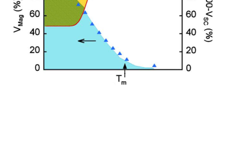
Figure 11: Nanoscopic coexistence of magnetism and superconductivity in CeFeAsO_0.94F_0.06 [94].

On the other hand, the cases of Ce- and Sm-based $1111$ oxy-pnictides were shown to be dramatically different from what observed in LaFeAsO_1-xF_x. In these materials, the coexistence region of magnetism and superconductivity was shown to be characterized by $V_{m}\simeq 100$ % with a bulk fraction of the sample being at the same time superconductor, as illustrated in Fig. 11 in the case of CeFeAsO_0.94F_0.06 [94]. These findings are interpreted by coming back to Fig. 9 and by now assuming that $d\sim 1-10$ nm. Under these circumstances, both $\mu_{1}^{+}$ and $\mu_{2}^{+}$ (namely, all the implanted $\mu^{+}$) probe static magnetism being the maximum distance between different magnetic domains of the same order of magnitude of $d$, namely the spatial range for the dipolar fields generated by domain walls. Accordingly, one has $V_{m}\simeq 100$ % and it must be assumed that the interstitial regions between the different magnetic domains are superconducting since dc magnetometry confirms that a bulk fraction of the sample contributes to the diamagnetic shielding. Such fine intertwining of different order parameters was detected in SmFeAsO_1-xF_x [99, 100, 101], in CeFeAsO_1-xF_x [94, 53], in CeFe_1-xCo_xAsO [55].

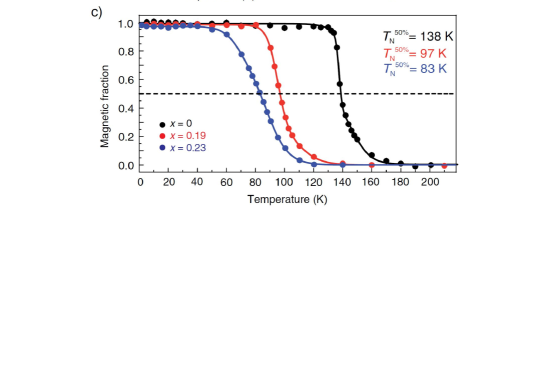
Figure 12: Nanoscopic coexistence of magnetism and superconductivity in Ba_1-xK_xFe₂As₂ (Figure reprinted from Ref. [104]. Copyright (2011) by the American Physical Society). Panel (a): superconducting shielding fractions. Panel (b): electronic phase diagram for Ba_1-xK_xFe₂As₂. Panel (c): magnetic volume fractions.

It should be remarked that the picture of mesoscopic segregation described above for the case of Ba_1-xK_xFe₂As₂ was modified after the investigation of samples with higher chemical homogeneity, displaying that the nanoscopic coexistence is a more suited framework for such materials [104]. At the sake of clarity, results relative to the hole-doped Ba_1-xK_xFe₂As₂ are reported in Fig. 12 [104]. It is rather interesting to observe that a static magnetic ground-state is recovered also by diluting optimally electron-doped $1111$ materials with Ru [44, 45]. Remarkably, the magnetic and superconducting ground-states coexist at the nanoscopic level and the latter one is completely suppressed for a Ru content around 60% (see Fig. 5). The observation of such a tiny effect of diamagnetic impurities on the superconducting transition temperature would appear at first in contrast with a magnetic pairing mechanism and has lead to alternative explanations, as the ones involving orbital currents [63, 64]. Still, it is possible that the subtle interplay between intraband and interband pairing processes can give rise to such a slow decrease of $T_{c}$ even in the framework of a magnetic pairing mechanism [102, 103]. Finally, it is important to point out that the different families of IBS show some significant differences. In Fig. 13 the phase diagram of Ba(Fe_1-xCo_x)₂As₂ [88] and of CeFe_1-xCo_xAsO [55] is reported. In spite of the quantitatively similar trend of the magnetic ordering temperature, which in the Ce-based 1111 compound was shown to be long-range for $x<0.03$ and short-range at higher doping levels [55], one notices clear differences at the crossover between the magnetic and the superconducting ground-states. In the 122 compound the coexistence region between the two phases is quite extended while in the 1111 compound it is only marginal. Moreover, the superconducting transition temperature is lower in the 1111 compounds. This suggests that the differences in the band structure, namely in the FS nesting, and in the anisotropy of the two family of compounds could play a relevant role in determining the superconducting properties, particularly when the charge doping is associated with the introduction of impurities in the FeAs planes.

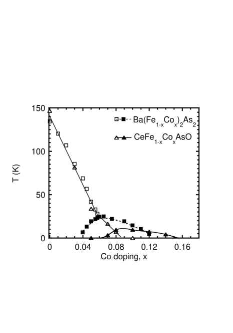
Figure 13: The phase diagram of Ba(Fe_1-xCo_x)₂As₂ [88] and of CeFe_1-xCo_xAsO [55] are reported as a function of the Co content $x$. Open symbols show the behaviour of $T_{N}(x)$ while the closed symbols show that of $T_{c}(x)$.

4 Transverse-field $\mu^{+}$SR in superconducting materials

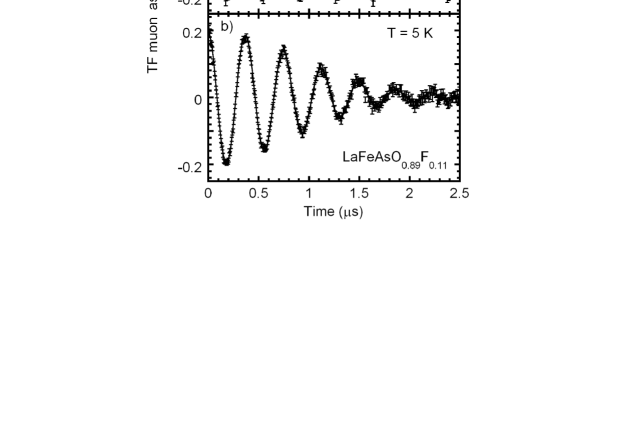
Figure 14: Representative time evolution of the TF-$\mu$SR asymmetry for a polycrystalline sample of LaFeAsO_0.89F_0.11 at T values well above and below the superconducting transition temperature $T_{c}=28$ K, performed in an external magnetic field $H_{0}=200$ G perpendicular to the initial muon spin polarization. Solid curves are best fits to a Gaussian damped precession (see text).

When type II superconductors, as the IBS, are field-cooled in an external field $H_{c1}<H_{0}<H_{c2}$ ($H_{0},H_{c1}$ and $<H_{c2}$ being the external, the lower and the upper critical field, respectively) the magnetic field is not homogeneously distributed throughout the sample but concentrated along tubes which form a FLL. Since the distance among two adjacent flux lines is much larger than the distance between the muon sites, the muons are able to finely probe the field distribution generated by the FLL. Such distribution leads to an enhancement of the muon depolarization rate which can be suitably probed in transverse field (TF) $\mu^{+}$SR experiments. The FLL field distribution is not symmetric around $H_{0}$ [16] since it reflects the minimum, the maximum and the saddle-point values of the magnetic field profile within the triangular FLL unit cell. In real samples, and in particular in powders, the FLL imperfections arising from randomly distributed pinning centers average out these asymmetries and the field distribution tends to a Gaussian one, centered around the average internal field $B_{\mu}$. Hence, the TF muon depolarization function can be approximated by $D_{TF}(t)\approx exp[-(\sigma_{SC}^{2}+(\sigma^{s}_{N})^{2})t^{2}/2]$, with $\sigma^{s}_{N}$ the weak relaxation due to the nuclear magnetic dipoles (see Eq. 2) and $\sigma_{SC}$ the second moment of the FLL field distribution, namely $\sigma_{SC}/\gamma_{\mu}=\!\!=\!\!(\overline{B}^{2}-{B_{\mu}^{2}})^{1/2}$. The latter term is proportional to the inverse square of the London penetration depth $\lambda_{L}$ and, in turn, to the supercarrier density $n_{s}$. Accordingly, one can write that $\sigma_{SC}(T)\propto n_{s}/m^{*}$ with $m^{*}$ the electron effective mass. Since each flux line is surrounded by a screening current over a distance of the order of $\lambda_{L}$, the average field at the muon site $B_{\mu}$ is slightly lower than the applied field, namely $B_{\mu}=(1+4\pi\chi)H_{0}$ with $\chi<0$.

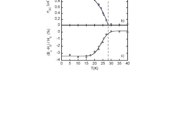
Figure 15: Superconducting response of LaFeAsO_0.89F_0.11 as a function of temperature. a) Zero field cooled (ZFC) and field cooled (FC) magnetic susceptibility, evaluated from magnetization measurements performed at $H=5$ Gauss by assuming a nearly spherical grain powders with demagnetization factor $N=4\pi/3$. b) Relaxation rate $\sigma_{SC}$ fitted using a standard BCS curve; the constant behavior at low T is indicative of a gap function without nodes. c) Relative shift of the magnetic field at the muon site $B_{\mu}$ respect to the applied field $H_{0}$. The lines in panel a) and c) are guides for the eye.

Fig. 14 shows the typical time evolution of the TF muon asymmetry $A_{TF}(t)$ in LaFeAsO_0.89F_0.11, measured at $T$ values above (a) and below (b) $T_{c}$= 28 K. The superconducting critical temperature was derived from the $T$-dependence of the magnetic susceptibility, $\chi(T)$, as shown in Fig 15(a). The $A_{TF}(t)$ data fit rather well to the function

$$\frac{A_{TF}(t)}{A_{TF}(0)}=a_{TF}\cdot exp[-(\sigma_{SC}^{2}+\sigma_{N}^{2})t^{2}/2]cos(\gamma_{\mu}B_{\mu}t)$$ (9)

throughout the whole temperature range $0<T<50$ K with a constant amplitude $a_{TF}$. This ensures that all the muons probe the same field distribution, i.e. the sample is always single phase and fully superconducting. The depolarization rate for $T>T_{c}$ is Gaussian and its rather low value, $\sigma_{N}=0.17\mu s^{-1}$, indicates that the amount of dilute magnetic impurities, which are often present in IBS and cause an unwanted enhancement in the relaxation rate [105, 99], is negligible in that sample. The temperature evolution of the FLL contribution to the depolarization rate, $\sigma_{SC}(T)$, and the relative shift of the field at the muon site, $\left(B_{\mu}(T)-H_{0}\right)/H_{0}$, due to the diamagnetic shielding are shown in Fig. 15(b) and (c), respectively. The development of the FLL is clearly evidenced both by the increase of $\sigma_{SC}$ and by the diamagnetic shift of $B_{\mu}$ below $T_{c}^{TF}=28K$, which coincide with that measured by $\chi(T)$. From the value of $\sigma_{SC}$ extrapolated at T=0, by using the relation $\sigma_{SC}=7.58\times 10^{-4}\lambda_{L}^{-2}$, in CGS units, [106, 107], the London penetration depth is estimated to be $\lambda_{L}\simeq 2620$ Å. The temperature dependence of $\sigma_{SC}(T)$ follows the s-wave weak coupling BCS temperature dependence predicted by the two fluid model $\sigma_{SC}(T)\propto 1/\lambda^{2}(T)\propto[1-(T/T_{c})^{4}]$, as shown by the curve in Fig. 15(b). In particular, the flat behavior for $T<T_{c}/3$ is indicative of the absence of nodes in the gap function.

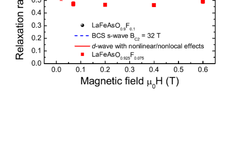
Figure 16: Field dependence of the muon relaxation rate $\sigma_{SC}$ at $T=1.6$ K for LaFeAsO_0.925F_0.075 and LaFeAsO_0.9F_0.1 powder samples with data fit to a d-wave (solid line) or s-wave (dashed line) behavior (Figure reprinted from Ref. [108]. Copyright (2008) by the American Physical Society).

The s-wave-like $T$-dependence of $\sigma_{SC}$ was also observed in a La-based 1111 compound with $T_{c}=23$ K [108]. However, this behavior is in conflict with the observed dependence of $\sigma_{SC}$ on the magnitude of the applied field $H_{0}$. In fact, as it is shown in Fig. 16 [108], $\sigma_{SC}$ displays a maximum for a field value $B^{max}\approx 200\div 2000$ G and at higher fields the relaxation rate decreases, which is usually indicative of superconductivity with nodes in the gap function [108, 109]. It should be noticed that this feature, also found in Sm-based 1111 compounds, could be rather due to the presence of different superconducting gaps [111], as it can be expected for system with several bands crossing the Fermi level. This field dependence should be carefully considered when comparing results from different experiments in the so-called Uemura like plot, where $T_{c}$ is plotted as a function of $\sigma_{SC}(T=0)\propto n_{s}(T=0)$. In Fig. 17 this behavior is shown for the 1111 family as a function of the F doping for those values of $\sigma_{SC}(T=0)$ measured at a field close to $B^{max}$. Although a theoretical description of the Uemura plot for the 1111 IBS is still missing, it is clear that the rate of the decrease of $T_{c}$ with $n_{s}(0)$ strongly depends on the symmetry of the order parameter, on the presence of nodes in the gap and on the occurrence of pair breaking processes. Hence, a suitable modeling of that plot would have significant implications in the clarification of the pairing mechanism for IBS. Nevertheless, it has also to be remarked that a temperature dependence of $\sigma_{SC}$ can be observed at low $T$ in underdoped La-based 1111 samples [110], leading to some uncertainty in the estimate of $\sigma_{SC}(T=0)$. Indeed, while analyzing the behavior of $\sigma_{SC}(T)$ a great care must be taken in order to discern those effects not associated with the $n_{s}$ $T$-dependence, as it will be described in the following section.

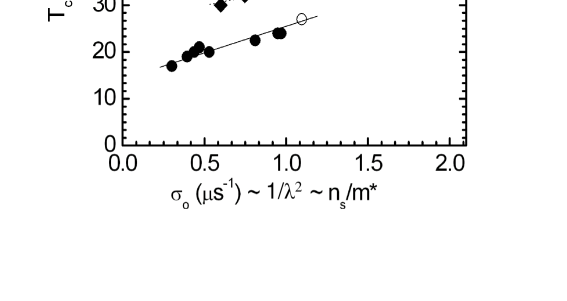
Figure 17: Uemura plot for 1111 families with different rare earth ions, with $\sigma_{SC}$ values measured in a transverse field $H_{0}\sim B^{max}$ (see text). Open and solid symbols are from this work and from Refs. [108, 98, 113, 114, 110, 100, 115], respectively.

5 Transverse-field $\mu^{+}$SR in case of coexistence between magnetism and superconductivity

In IBS, two main effects might alter the TF depolarization rates. One is extrinsic and comes from diluted ferromagnetic impurities which are often present in polycrystalline samples. These can be recognized in ZF experiments by an exponential depolarization either of the TF-muon asymmetry for $T>T_{c}$ or of the ZF-muon asymmetry spectrum for $T>T_{N}$. In TF-$\mu^{+}$SR experiments, this exponential term sometimes can be subtracted after a calibration above $T_{c}$ and kept constant over the whole temperature range, even if this procedure might be affected by some error due to the field/temperature dependence of the spurious magnetic contribution. Another important effect might originate from the presence of a static order or of magnetic correlations developing close to it, especially in underdoped compounds or when magnetic rare earths are present. In particular, when a static order appears the corresponding spontaneous internal fields $B_{i}$ add to $H_{0}$ and the muons detect a local field $B_{mag}\approx|$H₀+ B_i$|$. Hence both the value of the internal fields and that of the depolarization rate are strongly enhanced. Their behavior depends on the distribution width of the internal fields $B_{i}$ which, in principle, requires a vectorial analysis to take into account the muon spin projection along the detector direction [112]. Under those circumstances, the information on the superconducting state is usually lost.

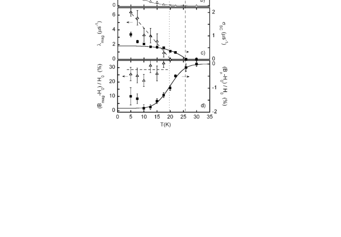
Figure 18: Zero field cooled (ZFC) and field cooled (FC) magnetic susceptibility, evaluated from magnetization measurements performed at $H=5$ G by assuming a nearly spherical grain powders with demagnetization factor $N=1/3$. b) Muon fractions $a_{mag}(T)$, probing nanoscopic regions with sizeable internal fields $B_{i}$ from the spontaneous Fe magnetic order, and $a_{SC}(T)$, where the superconducting FLL distribution is almost unperturbed. c) Relaxation rate of the muon asymmetry and d) relative shift of the magnetic field at the muon site respect to the applied field $H_{0}$, for the magnetic (left axis) and non magnetic (right axis) contributions. All the lines are guides for the eye.

In the 1111 compounds, where magnetism and superconductivity coexist at the nanoscopic level, $B_{i}$ ranges from a maximum field of few hundreds of Gauss to nearly zero, since it originates from ordered moments varying over distance from less than one to four-five lattice steps. In this case, one may assume that a fraction of the muons experiences internal fields lowered by $4\pi|\chi|H_{0}$. Then, the typical TF signal of the FLL is roughly distinguishable, even if it is still slightly affected by the nearby $B_{i}$ which give rise to a moderate increase both of $B_{\mu}(T)$ and of $\sigma_{SC}(T)$. For example, here the behavior of a NdFe_0.8Ru_0.2AsO_0.89F_0.11 powder sample is considered. This sample has $T_{c}=26$ K (Fig 18(a)) and by ZF muon experiments it was shown to display a magnetic transition with an onset at $T_{N}^{onset}\approx 20$ K and a full magnetic volume fraction $V_{m}\simeq 1$ below $T=5$ K, with internal fields at the muon site of the order of 200 G (see Fig. 1 of Ref. [45]). The TF asymmetry data (not shown) fit quite well to the sum of two oscillating terms

$$\frac{A_{TF}(t)}{A_{TF}(0)} = a_{SC}\cdot exp(-\Lambda t)\cdot exp[-(\sigma_{SC}^{2})t^{2}/2]\cdot cos(\gamma_{\mu}B_{\mu}t)$$ (10)

$$+ a_{mag}\cdot exp[-\lambda_{mag}t]\cdot cos(\gamma_{\mu}B_{mag}t)\,\,\,,$$

where the first accounts for those regions with vanishing $B_{i}$, where the field distribution still reflects the FLL for $T>T_{N}^{onset}$, while the second one accounts for those regions where the spontaneous internal field is of the order of $H_{0}$. The $\Lambda$ decay rate takes into account the exponential decay measured already at high temperature, close to the value $\Lambda\simeq 0.8\mu s^{-1}$ and nearly temperature independent, which is most probably due to the presence of a small fraction of diluted magnetic impurities. The temperature dependence of the TF parameters is shown in Fig. 18. Superconductivity is well reflected by the behavior both of the increase of $\sigma_{SC}(T)$ and of the diamagnetic shift (right axis of panels c and d, respectively) below the same $T_{c}$ determined by the $\chi(T)$ curve. At low temperature they both deviate from the behavior expected for a single SC phase compound, roughly for $T<10$ K where the ZF experiment displays a sizeable magnetic volume fraction [45], confirming the nanoscopic character of the coexistence. The panel Fig 18(b) shows that the $a_{SC}/a^{0}_{TF}$ fraction is close the unity in the temperature range $T_{N}^{onset}<T<T_{c}$, namely the full sample is in the superconducting phase. Below $T_{N}^{onset}\approx 20$ K, which agrees with the ZF measurements reported in Fig. 1 of Ref. [45], the regions where the spontaneous fields sum to the external one are signaled by the increase of the muon fraction $a_{mag}$ displaying the field at the muon site $B_{mag}>H_{0}$ (left axis of Fig 18(d)) and high values of the depolarization rate $\lambda_{mag}$ (left axis of Fig 18(c)) which grows according to the increase of the magnetic volume fraction.

6 Summarizing Remarks

Only five years after the discovery of superconductivity in the Fe pnictides, $\mu^{+}$SR experiments have allowed to reach several relevant milestones in the understanding of the microscopic properties of IBS. As shown in Sect. 3, thanks to its sensitivity to the magnetic order, even when it is short range, $\mu^{+}$SR has played a crucial role in the description of the phase diagram of the IBS, in the understanding of the phase transition between the magnetic and the superconducting phases and of their possible coexistence at the nanoscopic level. The TF-$\mu^{+}$SR studies reported in Sect. 4, performed in the mixed phase where the FLL sets in, have provided a description of the evolution of the superconducting carrier density $n_{s}$ as one spans through the phase diagram of IBS and shown how this quantity is correlated with $T_{c}$. The behaviour of $n_{s}(T)$ and of $n_{s}(T\rightarrow 0)$ vs $T_{c}$ have given relevant hints on the symmetry of the superconducting order parameter and on the microscopic mechanisms underlying the superconductivity in IBS. A remarkable experimental effort is still required to have a clear understanding of the physics of IBS and to distinguish the peculiarities of each family of compounds from the relevant features underlying a common description of the superconducting condensate.

7 Acknowledgements

We would like to thank all those colleagues who have recently collaborated with us in the realization of the $\mu$SR experiments in the IBS. In particular: Alex Amato, Pietro Bonfà, Lucia Bossoni, Sean Giblin, Rustem Khasanov, Gianrico Lamura, Hubertus Luetkens, Marcello Mazzani and Toni Shiroka. Pietro Carretta and Samuele Sanna also acknowledge the financial support from Fondazione Cariplo (research grant no. 2011-0266) for the research activity on IBS. Giacomo Prando acknowledges support from the Leibniz-Deutscher Akademischer Austauschdienst (DAAD)Post-Doc Fellowship Program

References

References

- [1] J. G. Bednorz, K. A. Müller, Z. Phys. B 64, 189 (1986)
- [2] P. A. Lee, N. Nagaosa, X.-G. Wen, Rev. Mod. Phys. 78, 17 (2006)
- [3] Y. Kamihara, T. Watanabe, M. Hirano, H. Hosono, Journ. Am. Chem. Soc. 130, 3296 (2008)
- [4] Z.-A. Ren, W. Lu, J. Yang, W. Yi, X.-L. Shen, Z.-C. Li, G.-C. Che, X.-L. Dong, L.-L. Sun, F. Zhou, and Z.-X. Zhao, Chin. Phys. Lett. 25, 2215 (2008)
- [5] Visit the site http://www.superconductivity.eu to have a nice overview on the fascinating world of superconductors
- [6] D. C. Johnston, Adv. Phys. 59, 803 (2010)
- [7] H. D. Lumsden, A. D. Christianson, Journ. Phys.: Cond. Matt. 22, 203203 (2010)
- [8] J. Paglione, R. L. Greene, Nat. Phys. 6, 645 (2010)
- [9] G. R. Stewart, Rev. Mod. Phys. 83, 1589 (2011)
- [10] D. N. Basov, A. V. Chubukov, Nat. Phys. 7, 272 (2011)
- [11] P. C. Canfield, S. L. Bud’ko, Annu. Rev. Condens. Matter Phys. 1, 27 (2010)
- [12] A. Rigamonti, F. Borsa, P. Carretta, Rep. Prog. Phys. 61, 1367 (1998)
- [13] N. P. Armitage, P. Fournier, R. L. Greene, Rev. Mod. Phys. 82, 2421 (2010)
- [14] A. A. Kordyuk, Low Temp. Phys., 38, 888 (2012)
- [15] G. Blatter, M. V. Feigel’man, V. B. Geshkenbein, A. I. Larkin, V. M. Vinokur, Rev. Mod. Phys. 66, 1125 (1994)
- [16] E. H. Brandt, Rep. Prog. Phys. 58, 1465 (1995)
- [17] G. Prando, P. Carretta, R. De Renzi, S. Sanna, A. Palenzona, M. Putti, M. Tropeano, Phys. Rev. B 83, 174514 (2011)
- [18] G. Prando, P. Carretta, R. De Renzi, S. Sanna, H.-J. Grafe, S. Wurmehl, B. Büchner, Phys. Rev. B 85, 144522 (2012)
- [19] G. Prando, R. Giraud, M. Abdel-Hafiez, S. Aswartham, A. U. B. Wolter, S. Wurmehl, B. Büchner, arXiv:1207.2457v2 (2012)
- [20] G. Prando, Phase diagrams of REFeAsO1-xFx materials: macroscopic and nanoscopic experimental investigation (Ph. D. Thesis), Aracne Editrice (2013)
- [21] L. Bossoni, P. Carretta, M. Horvatić, M. Corti, A. Thaler, P. C. Canfield, Europhys. Lett. 102, 17005 (2013)
- [22] F. Hunte, J. Jaroszynski, A. Gurevich, D. C. Larbalestier, R. Jin, A. S. Sefat, M. A. McGuire, B. C. Sales, D. K. Christen, D. Mandrus, Nature 453, 903 (2008)
- [23] G. Fuchs, S.-L. Drechsler, N. Kozlova, M. Bartkowiak, J. E. Hamann-Borrero, G. Behr, K. Nenkov, H.-H. Klauss, H. Maeter, A. Amato, H. Luetkens, A. Kwadrin, R. Khasanov, J. Freudenberger, A. Köhler, M. Knupfer, E, Arushanov, H. Rosner, B. Büchner, L. Schultz, New Journ. Phys. 11, 075007 (2009)
- [24] I. I. Mazin, Nature 464, 183 (2010)
- [25] D. J. Singh, M.-H. Du, Phys. Rev. Lett. 100, 237003 (2008)
- [26] D. J. Singh, Phys. Rev. B 78, 094511 (2008)
- [27] A. Subedi, L. Zhang, D. J. Singh, M. H. Du, Phys. Rev. B 78, 134514 (2008)
- [28] B. Batlogg, H. Y. Hwang, H. Takagi, R. J. Cava, H. L. Kao, J. Kwo, Physica C 235 - 240, 130 (1994)
- [29] Q. Si, E. Abrahams, Phys. Rev. Lett. 101, 076401 (2008)
- [30] Q. Si, E. Abrahams, J. Dai, J.-X. Zhu, New. Journ. Phys. 11, 045001 (2009)
- [31] M. M. Qazilbash, J. J. Hamlin, R. E. Baumbach, L. Zhang, D. J. Singh, M. B. Maple, D. N. Basov, Nat. Phys. 5, 647 (2009)
- [32] M. D. Johannes, I. I. Mazin, Phys. Rev. B 79, 220510 (2009)
- [33] I. I. Mazin, J. Schmalian, Phys. C 469, 614 (2009)
- [34] T. Yildrim, Phys. Rev. Lett. 101, 057010 (2008)
- [35] A. Smerald, N. Shannon, Europhys. Lett. 92, 47005 (2010)
- [36] P. Bonfà, P. Carretta, S. Sanna, G. Lamura, G. Prando, A. Martinelli, A. Palenzona, M. Tropeano, M. Putti, R. De Renzi, Phys. Rev. B 85, 054518 (2012)
- [37] H. Wadati, I. Elfimov, and G. A. Sawatzky, Phys. Rev. Lett. 105, 157004 (2010)
- [38] T. Berlijn, C.-H. Lin, W. Garber, and W. Ku, Phys. Rev. Lett. 108, 207003 (2012)
- [39] E. M. Bittar, C. Adriano, T. M. Garitezi, P. F. S. Rosa, L. Mendonça-Ferreira, F. Garcia, G. de M. Azevedo, P. G. Pagliuso, and E. Granado, Phys. Rev. Lett. 107, 267402 (2011)
- [40] M. Merz, F. Eilers, T. Wolf, P. Nagel, H. v. Löhneysen, and S. Schuppler, Phys. Rev. B 86, 104503 (2012)
- [41] G. Levy, R. Sutarto, D. Chevrier, T. Regier, R. Blyth, J. Geck, S. Wurmehl, L. Harnagea, H. Wadati, T. Mizokawa, I. S. Elfimov, A. Damascelli, and G. A. Sawatzky, Phys. Rev. Lett. 109, 077001 (2012)
- [42] A. Thaler, N. Ni, A. Kracher, J. Q. Yan, S. L. Bud’ko, P. C. Canfield, Phys. Rev. B 82, 014534 (2010)
- [43] R. S. Dhaka, C. Liu, R. M. Fernandes, R. Jiang, C. P. Strehlow, T. Kondo, A. Thaler, J. Schmalian, S. L. Bud’ko, P. C. Canfield, A. Kaminski, Phys. Rev. Lett. 107, 267002 (2011)
- [44] S. Sanna, P. Carretta, P. Bonfà, G. Prando, G. Allodi, R. De Renzi, T. Shiroka, G. Lamura, A. Martinelli, M. Putti, Phys. Rev. Lett. 107, 227003 (2011)
- [45] S. Sanna, P. Carretta, R. De Renzi, G. Prando, P. Bonfà, M. Mazzani, G. Lamura, T. Shiroka, Y. Kobayashi, M. Sato, Phys. Rev. B 87, 134518 (2013)
- [46] H. Takahashi, K. Igawa, K. Arii, Y. Kamihara, M. Hirano, H. Hosono, Nature 453, 376 (2008)
- [47] C. W. Chu, B. Lorenz, Phys. C 469, 385 (2009)
- [48] R. Khasanov, S. Sanna, G. Prando, Z. Shermadini, M. Bendele, A. Amato, P. Carretta, R. De Renzi, J. Karpinski, S. Katrych, H. Luetkens, N. D. Zhigadlo, Phys. Rev. B 84, 100501 (2011)
- [49] E. Gati, S. Köhler, D. Guterding, B. Wolf, S. Knöner, S. Ran, S. L. Bud’ko, P. C. Canfield, M. Lang, Phys. Rev. B 86, 220511 (2012)
- [50] C. Wang, S. Jiang, Q. Tao, Z. Ren, Y. Li, L. Li, C. Feng, J. Dai, G. Cao, X.-A. Xu, Europhys. Lett. 86, 47002 (2009)
- [51] G. Prando, P. Carretta, A. Rigamonti, S. Sanna, A. Palenzona, M. Putti, M Tropeano, Phys. Rev., B 81, 100508 (2010)
- [52] L. Pourovskii, V. Vildosola, S. Biermann, A. Georges, Europhys. Lett. 84, 37006 (2008)
- [53] T. Shiroka, G. Lamura, S. Sanna, G. Prando, R. De Renzi, M. Tropeano, M. R. Cimberle, A. Martinelli, C. Bernini, A. Palenzona, R. Fittipaldi, A. Vecchione, P. Carretta, A. S. Siri, C. Ferdeghini, M. Putti, Phys. Rev. B 84, 195123 (2011)
- [54] H. Maeter, J. E. Hamann Borrero, T. Goltz, J. Spehling, A. Kwadrin, A. Kondrat, L. Veyrat, G. Lang, H.-J. Grafe, C. Hess, G. Behr, B. Büchner, H. Luetkens, C. Baines, A. Amato, N. Leps, R. Klingeler, R. Feyerherm, D. Argyriou, H.-H. Klauss, arXiv:1210.6959 (2012)
- [55] G. Prando, O. Vakaliuk, S. Sanna, G. Lamura, T. Shiroka, P. Bonfà, P. Carretta, R. De Renzi, H.-H. Klauss, S. Wurmehl, C. Hess, B. Büchner, Phys. Rev. B 87, 174519 (2013)
- [56] D. A. Zocco, R. E. Baumbach, J. J. Hamlin, M. Janoschek, I. K. Lum, M. A. McGuire, A. S. Sefat, B. C. Sales, R. Jin, D. Mandrus, J. R. Jeffries, S. T. Weir, Y. K. Vohra, M. B. Maple, Phys. Rev. B 83, 094528 (2011)
- [57] A. Jesche, T. Förster, J. Spheling, M. Nicklas, M. de Souza, R. Gumeniuk, H. Luetkens, T. Goltz, C. Krellner, M. Lang, J. Sichelschmidt, H.-H. Klauss, C. Geibel, Phys. Rev. B 86, 020501 (2012)
- [58] K. Jin, N. P. Butch, K. Kirshenbaum, J. Paglione, R. L. Greene, Nature 476, 73 (2011)
- [59] J. Mannhart, H. Hilgenkamp, G. Hammerl, C. W. Schneider, Phys. Scr. T 102, 107 (2002)
- [60] S. R. Park, D. J. Song, C. S. Leem, C. Kim, C. Kim, B. J. Kim, H. Eisaki, Phys. Rev. Lett. 101, 117006 (2008)
- [61] I. I. Mazin, D. J. Singh, M. D. Johannes, M. H. Du, Phys. Rev. Lett. 101, 057003 (2008)
- [62] G. A. Ummarino, Phys. Rev. B 83, 092508 (2011)
- [63] H. Kontani, S. Onari, Phys. Rev. Lett. 104, 157001 (2010)
- [64] S. Onari, H. Kontani, Phys. Rev. Lett. 109, 137001 (2012)
- [65] L. Boeri, O. V. Dolgov, A. A. Golubov, Phys. Rev. Lett. 101, 026403 (2008)
- [66] Y. J. Uemura, G. M. Luke, B. J. Sternlieb, J. H. Brewer, J. F. Carolan, W. N. Hardy, R. Kadono, J. R. Kempton, R. F. Kiefl, S. R. Kreitzman, P. Mulhern, T. M. Riseman, D. L. Williams, B. X. Yang, S. Uchida, H. Takagi, J. Gopalakrishnan, A. W. Sleight, M. A. Subramanian, C. L. Chien, M. Z. Cieplak, G. Xiao, V. Y. Lee, B. W. Statt, C. E. Stronach, W. J. Kossler, X. H. Yu, Phys. Rev. Lett. 62, 2317 (1989)
- [67] J. E. Sonier, Rep. Prog. Phys. 70, 1717 (2007)
- [68] S. F. J. Cox, Journ. Phys. C, 20, 3187 (1987)
- [69] P. Dalmas de Réotier, A. Yaouanc, Journ. Phys. Cond. Matt., 9, 9113 (1997)
- [70] S. J. Blundell, Contemporary Physics 40, 175 (1999)
- [71] J. E. Sonier, J. H. Brewer, R. F. Kiefl, Rev. Mod. Phys. 72, 769 (2000)
- [72] A. Yaouanc, P. Dalmas de Réotier, Muon Spin Rotation, Relaxation, and Resonance, Oxford Science Publications (2011)
- [73] G. Lang, H.-J. Grafe, D. Paar, F. Hammerath, K. Manthey, G. Behr, J. Werner, B. Büchner, Phys. Rev. Lett. 104, 097001 (2010)
- [74] R. Khasanov, K. Conder, E. Pomjakushina, A. Amato, C. Baines, Z. Bukowski, J. Karpinski, S. Katrych, H.-H. Klauss, H. Luetkens, A. Shengelaya, and N. D. Zhigadlo Phys. Rev. B 78, 220510 (2008)
- [75] M. Bendele, A. Amato, K. Conder, M. Elender, H. Keller, H.-H. Klauss, H. Luetkens, E. Pomjakushina, A. Raselli, and R. Khasanov Phys. Rev. Lett. 104, 087003 (2010)
- [76] R. Khasanov, M. Bendele, A. Amato, K. Conder, H. Keller, H.-H. Klauss, H. Luetkens, and E. Pomjakushina Phys. Rev. Lett. 104, 087004 (2010)
- [77] M. Bendele, S. Weyeneth, R. Puzniak, A. Maisuradze, E. Pomjakushina, K. Conder, V. Pomjakushin, H. Luetkens, S. Katrych, A. Wisniewski, R. Khasanov, and H. Keller Phys. Rev. B 81, 224520 (2010)
- [78] Z. Shermadini, A. Krzton-Maziopa, M. Bendele, R. Khasanov, H. Luetkens, K. Conder, E. Pomjakushina, S. Weyeneth, V. Pomjakushin, O. Bossen, and A. Amato Phys. Rev. Lett. 106, 117602 (2011)
- [79] M. Bendele, A. Ichsanow, Yu. Pashkevich, L. Keller, Th. Strässle, A. Gusev, E. Pomjakushina, K. Conder, R. Khasanov, and H. Keller Phys. Rev. B 85, 064517 (2012)
- [80] P. K. Biswas, A. Krzton-Maziopa, R. Khasanov, H. Luetkens, E. Pomjakushina, K. Conder, and A. Amato Phys. Rev. Lett. 110, 137003 (2013)
- [81] F. L. Pratt, P. J. Baker, S. J. Blundell, T. Lancaster, H. J. Lewtas, P. Adamson, M. J. Pitcher, D. R. Parker, and S. J. Clarke Phys. Rev. B 79, 052508 (2009)
- [82] T. Wu, H. Mayaffre, S. Krämer, M. Horvatic, C. Berthier, W. N. Hardy, R. Liang, D. A. Bonn, M.-H. Julien, Nature 477, 191 (2011)
- [83] H.-J. Grafe, Physica C 481, 93 (2012)
- [84] R. De Renzi, P. Bonfà, M. Mazzani, S. Sanna, G. Prando, P. Carretta, R. Khasanov, A. Amato, H. Luetkens, M. Bendele, F. Bernardini, S. Massidda, A. Palenzona, M. Tropeano, M. Vignolo, Supercond. Sci. Technol. 25, 084009 (2012)
- [85] G. Prando, P. Bonfà, G. Profeta, R. Khasanov, F. Bernardini, M. Mazzani, E. M. Brüning, A. Pal, V. P. S. Awana, H.-J. Grafe, B. Büchner, R. De Renzi, P. Carretta, S. Sanna, Phys. Rev. B 87, 064401 (2013)
- [86] H. Maeter, H. Luetkens, Yu. G. Pashkevich, A. Kwadrin, R. Khasanov, A. Amato, A. A. Gusev, K. V. Lamonova, D. A. Chervinskii, R. Klingeler, C. Hess, G. Behr, B. Büchner, H.-H. Klauss, Phys. Rev. B 80, 094524 (2009)
- [87] H.-H. Klauss, H. Luetkens, R. Klingeler, C. Hess, F. J. Litterst, M. Kraken, M. M. Korshunov, I. Eremin, S.-L. Drechsler, R. Khasanov, A. Amato, J. Hamann-Borrero, N. Leps, A. Kondrat, G. Behr, J. Werner, B. Büchner, Phys. Rev. Lett. 101, 077005 (2008)
- [88] C. Bernhard, C. N. Wang, L. Nuccio, L. Schulz, O. Zaharko, J. Larsen, C. Aristizabal, M. Willis, A. J. Drew, G. D. Varma, T. Wolf, C. Niedermayer, Phys. Rev. B 86, 184509 (2012)
- [89] C. Liu, G. D. Samolyuk, Y. Lee, N. Ni, T. Kondo, A. F. Santander-Syro, S. L. Bud’ko, J. L. McChesney, E. Rotenberg, T. Valla, A. V. Fedorov, P. C. Canfield, B. N. Harmon, A. Kaminski, Phys. Rev. Lett. 101, 177005 (2008)
- [90] J. P. Carlo, Y. J. Uemura, T. Goko, G. J. MacDougall, J. A. Rodriguez, W. Yu, G. M. Luke, P. Dai, N. Shannon, S. Miyasaka, S. Suzuki, S. Tajima, G. F. Chen, W. Z. Hu, J. L. Luo, N. L. Wang, Phys. Rev. Lett. 102, 087001 (2008)
- [91] R. M. Fernandes, D. K. Pratt, W. Tian, J. Zarestky, A. Kreyssig, S. Nandi, M. G. Kim, A. Thaler, N. Ni, P. C. Canfield, R. J. McQueeney, J. Schmalian, A. I. Goldman, Phys. Rev. B 81, 140501 (2010)
- [92] R. M. Fernandes, J. Schmalian, Phys. Rev. B 82, 014521 (2010)
- [93] J. T. Park, D. S. Inosov, C. Niedermayer, G. L. Sun, D. Haug, N. B. Christensen, R. Dinnebier, A. V. Boris, A. J. Drew, L. Schulz, T. Shapoval, U. Wolff, V. Neu, X. Yang, C. T. Lin, B. Keimer, V. Hinkov, Phys. Rev. Lett. 102, 117006 (2009)
- [94] S. Sanna, R. De Renzi, T. Shiroka, G. Lamura, G. Prando, P. Carretta, M. Putti, A. Martinelli, M. R. Cimberle, M. Tropeano, A. Palenzona, Phys. Rev. B 82, 060508 (2010)
- [95] G. Prando, S. Sanna, G. Lamura, T. Shiroka, M. Tropeano, A. Palenzona, H.-J. Grafe, B. Büchner, P. Carretta, R. De Renzi, Phys. Status Solidi B 250, 599 (2013)
- [96] Y. Laplace, J. Bobroff, F. Rullier-Albenque, D. Colson, A. Forget, Phys. Rev. B 80, 140501 (2009)
- [97] D. K. Pratt, W. Tian, A. Kreyssig, J. L. Zarestky, S. Nandi, N. Ni, S. L. Bud’ko, P. C. Canfield, A. I. Goldman, R. J. McQueeney, Phys. Rev. Lett. 103, 087001 (2009)
- [98] H. Luetkens, H.-H. Klauss, M. Kraken, F. J. Litterst, T. Dellmann, R. Klingeler, C. Hess, R. Khasanov, A. Amato, C. Baines, M. Kosmala, O. J. Schumann, M. Braden, J. Hamann-Borrero, N. Leps, A.Kondrat, G. Behr, J. Werner, B. Büchner, Nature Mat. 8, 305 (2009)
- [99] S. Sanna, R. De Renzi, G. Lamura, C. Ferdeghini, A. Palenzona, M. Putti, M. Tropeano, T. Shiroka, Phys. Rev. B 80, 052503 (2009)
- [100] A. J. Drew, F. L. Pratt, T. Lancaster, S. J. Blundell, P. J. Baker, R. H. Liu, G. Wu, X. H. Chen, I. Watanabe, V. K. Malik, A. Dubroka, K.W. Kim, M. Rössle, C. Bernhard, Phys. Rev. Lett. 101, 097010 (2008)
- [101] A. J. Drew, C. Niedermayer, P. J. Baker, F. L. Pratt, S. J. Blundell, T. Lancaster, R. H. Liu, G. Wu, X. H. Chen, I. Watanabe, V. K. Malik, A. Dubroka, M. Rössle, K. W. Kim, C. Baines, C. Bernhard, Nature Mat. 8, 310 (2009)
- [102] M. G. Vavilov, A. V. Chubukov, Phys. Rev. B 84, 214521 (2011)
- [103] R. M. Fernandes, M. G. Vavilov, A. V. Chubukov, Phys. Rev. B 85, 140512 (2012)
- [104] E. Wiesenmayer, H. Luetkens, G. Pascua, R. Khasanov, A. Amato, H. Potts, B. Banusch, H.-H. Klauss, D. Johrendt, Phys. Rev. Lett. 107, 237001 (2011)
- [105] P. K. Biswas, G. Balakrishnan, D. M. Paul, C. V. Tomy, M. R. Lees, and A. D. Hillier, Phys. Rev. B 81, 092510 (2010).
- [106] W. Barford and J. Gunn, Physica C 156, 515 (1988);
- [107] S.Sanna, F. Coneri, A. Rigoldi, G. Concas, R. De Renzi, Phys. Rev. B 77, 224511 (2008)
- [108] H. Luetkens, H.-H. Klauss, R. Khasanov, A. Amato, R. Klingeler, I. Hellmann, N. Leps, A. Kondrat, C. Hess, A. Köhler, G. Behr, J. Werner, and B. Büchner, Phys. Rev. Lett. 101, 097009 (2008).
- [109] J. E. Sonier, J.H. Brewer, and R. F. Kiefl, Rev. Mod. Phys. 72, 769 (2000).
- [110] S. Takeshita and R. Kadono, New J. Phys. 11, 035006 (2009).
- [111] S. Weyeneth, M. Bendele, R. Puzniak, F. Mur´anyi, A. Bussmann-Holder, N. D. Zhigadlo, S. Katrych, Z. Bukowski, J. Karpinski, A. Shengelaya, R. Khasanov and H. Keller, Europhys. Lett. 91, 47005 (2010).
- [112] G. Allodi, S. Sanna, G. Concas, R. Caciuffo, R. De Renzi, Physica B 374-375, 221 (2006).
- [113] J. P. Carlo, Y. J. Uemura, T. Goko, G. J. MacDougall, J. A. Rodriguez, W. Yu, G. M. Luke, Pengcheng Dai, N. Shannon, S. Miyasaka, S. Suzuki, S. Tajima, G. F. Chen, W. Z. Hu, J. L. Luo, and N. L. Wang, Phys. Rev. Lett. 102, 087001 (2009).
- [114] R. Khasanov, H. Luetkens, A. Amato, H.-H. Klauss, Z.-A. Ren, J. Yang, W. Lu, Z.-X. Zhao, Phys. Rev. B. 78, 092506 (2008).
- [115] H. Maeter, J. E. Hamann-Borrero, Ti. Goltz, J. Spehling, A. Kwadrin, A. Kondrat, L. Veyrat, G. Lang, H.-J. Grafe, C. Hess, G. Behr, B. Büchner, H. Luetkens, C. Baines, A. Amato, N. Leps, R. Klingeler, R. Feyerherm, D. Argyriou, and H.-H. Klauss, arXiv:1210.6959v1.