Detecting Local Deflection Patterns of Ultra-high Energy Cosmic Rays using the Principal Axes of the Directional Energy Distribution

Abstract

From deflections in galactic and extragalactic magnetic fields energy dependent structures in the arrival directions of ultra-high energy cosmic rays (UHECR) are expected. We propose to characterize these structures by the strength of collimation of energy along the principal axes in selected regions in the sky. While the strength of collimation are indicators of anisotropy in the arrival distribution of UHECR, the orientation of the principal system holds information about the direction of the deflections of UHECR. We discuss the method and present expected limits on the strength of deflection and density of sources using simulated scenarios of UHECR proton propagation.

1 Introduction

Ultra-high energy cosmic rays (UHECR) are likely accelerated in extragalactic point sources. Identifying such sources has not been successful so far, presumably due to the deflection of the charged cosmic rays in the galactic and extragalactic magnetic fields. However, the deflection of UHECR during their propagation can be quantitatively modelled using simulation software (e.g. [1, 2, 3, 4, 5]). To compare the predictions of the models with the datasets collected by experiments like the Pierre Auger Observatory [6, 7] or Telescope Array [8, 9], observables are needed that discriminate between different astrophysical scenarios. In particular, analysis of the energy and arrival directions of UHECR can probe cosmic magnetic fields and the density of sources of UHECR [10, 11, 12]. The expected deflection patterns can be abstracted as symmetric ‘blurring’ from multiple scattering in turbulent fields and threadlike structures from deflection in coherent fields. In a localized region in the sky, further on denoted as region of interest (ROI), both effects result in a collimation of energy along the axes of the principal system of the directional energy distribution.

2 The Thrust Observables

To derive the principal axes and quantify the collimation of energy along these axes, we use here the ‘thrust observables’ that were first used in high energy physics to characterize the energy distribution in particle collisions [13]. The three thrust observables $T_{k=1,2,3}$ quantify the strength of the collimation of the particle momenta along each of the three axes $\vec{n}_{k=1,2,3}$ of the principal system. The principal axes and the corresponding observables $T_{k}$ are successively determined by maximizing $T_{k}$ with respect to the axis $\vec{n}_{k}$ using

$$T_{k}=\max_{\vec{n}_{k}}\left(\frac{\sum_{i}|\vec{p}_{i}\vec{n}_{k}|}{\sum_{i}|\vec{p}_{i}|}\right)$$ (1)

with $\vec{p}_{i}$ being the momentum of the individual particles. For $k=1$ the quantity $T_{1}$ is called ‘thrust’ and consequently the first axis of the principal system $\vec{n}_{1}$ is called ‘thrust axis’. For the second axis the additional side condition $\vec{n}_{1}\perp\vec{n}_{2}$ is used in eq. 1. The resulting value $T_{2}$ is denoted as ‘thrust major’, the axis as ‘thrust major axis’. Finally, the third quantity $T_{3}$ is called ‘thrust minor’ with corresponding ‘thrust minor axis’. For the thrust minor axis $\vec{n}_{3}$ it is $\vec{n}_{1}\perp\vec{n}_{2}\perp\vec{n}_{3}$ which renders the maximization in eq. 1 trivial.

To use these observables in astroparticle physics, we calculate them from the momenta $\vec{p}_{i}$ of all events in a small circular region of the sky. As all observed cosmic rays approach the observer centered in the coordinate system, the thrust axis points to the barycenter of the energy distribution in this region. In spherical coordinates, the thrust axis is anti-parallel to the radial unit vector $\vec{e}_{r}$ pointing to the local barycenter of the energy distribution. The thrust major and thrust minor axes can therefore be written as linear combinations of the unit vectors $\vec{e}_{\phi}$ and $\vec{e}_{\theta}$ reading

$$\vec{n}_{2,3}=\cos{\xi_{2,3}}\cdot\vec{e}_{\phi}+\sin{\xi_{2,3}}\cdot\vec{e}_{\theta}$$ (2)

with $\xi_{3}=90^{\circ}+\xi_{2}$. Using this together with eq. 1, $T_{2}$ becomes maximal if $\vec{n}_{2}$ is aligned to a linear distribution of UHECR. The thrust major axis thus points along threadlike structures in the energy distribution of UHECR. As the thrust minor axis $\vec{n}_{3}$ is chosen perpendicular to $\vec{n}_{1}$ and $\vec{n}_{2}$ its direction has no physical meaning beyond its connection to the thrust major axis. The corresponding thrust minor value $T_{3}$ holds additional information beyond the values of $T_{1}$ and $T_{2}$.

We include all cosmic rays with energy above $E_{\min}=$5\text{\,}\mathrm{EeV}$$ in the calculations and set the radius of the circular region of interest to $\beta=$0.25\text{\,}\mathrm{rad}$$. These values have been chosen to maximize the discriminating power of propagation simulations from isotropic distributions of UHECR [14].

3 Example simulation

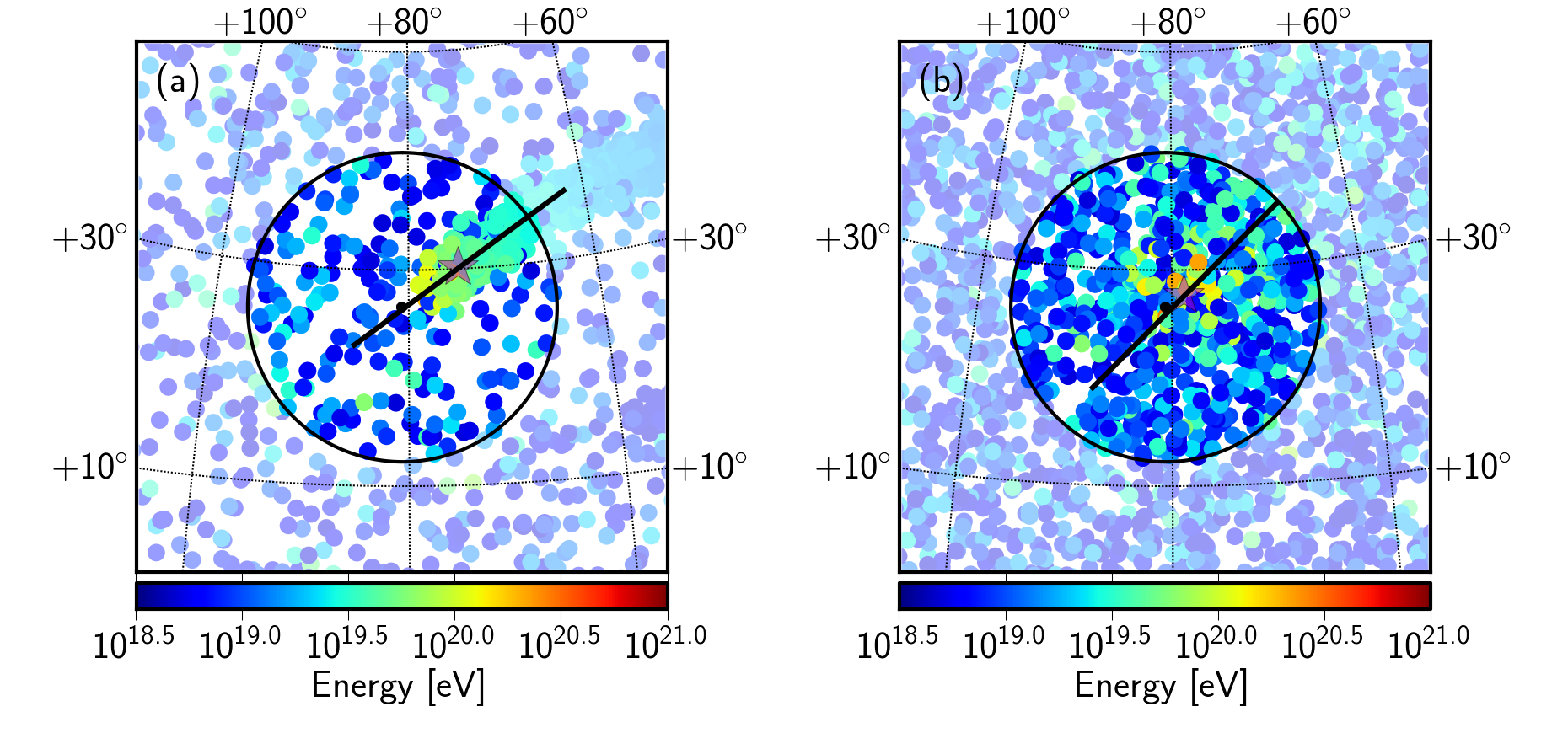
Figure 1: Region of interest around the closest source in two simulations with different strength of the EGMF $B=$0.1\text{\,}\mathrm{nG}$$ (left panel) and $B=$5\text{\,}\mathrm{nG}$$ (right panel). Colored dots denote arrival direction and energy of the UHECR. Source position, source density, and galactic magnetic field model are identical in both simulations. The thrust axis in the regions is denoted by a magenta star; the thrust major axis in this region is denoted by a black line.

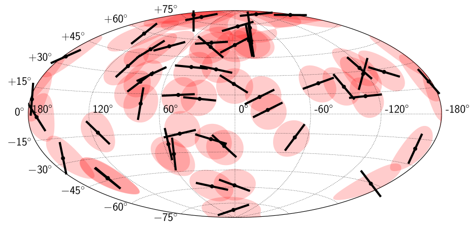
Figure 2: Typical skymap in galactic coordinates of thrust major axes (black lines) from anisotropically distributed UHECR from a PARSEC simulation with $0.1\text{\,}\mathrm{nG}$ extragalactic magnetic field, source density ${10}^{-5}\text{\,}{\mathrm{Mpc}}^{-3}$, and JF2012 model for the galactic magnetic field. Red shaded areas denote the individual ROI.

To demonstrate the thrust observables, we simulated 20 000 UHECR protons from homogeneously distributed point sources with a density $1\text{\times}{10}^{-5}\text{\,}{\mathrm{Mpc}}^{-3}$ in two scenarios with strengths of the extragalactic magnetic field $B=$0.1\text{\,}\mathrm{nG}$$ and $B=$5\text{\,}\mathrm{nG}$$ using the PARSEC software [4]. The galactic magnetic field is modeled using a lens for the regular component of the JF2012 [15] magnetic field. The position of the sources is identical in both simulations. All sources are simulated with equal luminosity, a power law spectrum with spectral index $\gamma=-2.7$, and a maximum energy of $1000\text{\,}\mathrm{EeV}$. Regions of interest with a size $\beta=$0.25\text{\,}\mathrm{rad}$$ are set to the closest 50 sources in the simulations.

In figure 1 the region around the closest source in the simulations is shown. A magenta star marks the direction of the thrust axis and a black line denotes the direction of the thrust major axis. For the weak extragalactic magnetic field shown in figure 1 (a), a tail of UHECR from the source resulting from coherent deflection is visible. The thrust major axis points along this structure. Because of the stronger deflections in the extragalactic magnetic field, the structure is not visible by eye in figure 1 (b). Nevertheless, the thrust major axis points in a similar direction in this example, indicating the preferred direction of deflection in the magnetic field. The values of thrust observable $T_{1}$ calculated in both cases deviates from the isotropic expectations by more than three times the spread of the corresponding isotropic distribution. Note that the observation of a single non-trivial ROI can be sufficient evidence for an anisotropic arrival distribution of UHECR. The complete map of thrust major axes of this example is shown in figure 2. The map indicates the deflection patterns of cosmic rays in the magnetic fields.

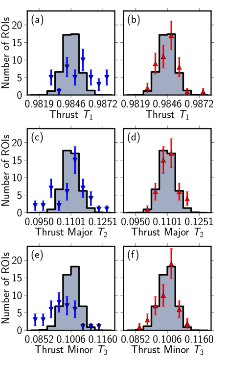
Figure 3: Distribution of observables $T_{1,2,3}$ in an example scenario using protons from homogeneously distributed point sources with density $\rho=$1\text{\times}{10}^{-4}\text{\,}\mathrm{M}\mathrm{pc}^{-3}$$, JF2012 regular galactic magnetic field, and strength of the extragalactic magnetic field (a,c,e) $B=$0.1\text{\,}\mathrm{nG}$$, and (b,d,f) $B=$5\text{\,}\mathrm{nG}$$. The gray histograms correspond to the average of the observables from 100 simulations with isotropically distributed UHECR.

In figure 3 the corresponding distributions of the observables $T_{1,2,3}$ are shown together with the mean of 100 simulations with isotropically distributed UHECR. For weak extragalactic magnetic fields, the distributions for $T_{1,2,3}$ deviate considerably in several ROI from the expectation for isotropically distributed UHECR. For $B=$5\text{\,}\mathrm{nG}$$, in this example only the thrust of a single ROI deviates from the isotropic expectation.

In the example above, we calculated the observables in regions centered at the sources of UHECR. As the sources of UHECR are, however, yet unknown, this is not possible in the analysis of measured data. In the analysis following below, we therefore choose regions around events with energy $E>$60\text{\,}\mathrm{EeV}$$ as ROI, assuming that UHECR with the highest energies are least deflected.

4 Statistical Interpretation

Searches for anisotropy and structure in the arrival directions of UHECR did not yet lead to strongly conclusive results. In order to exploit the sensitivity of our method to non-trivial astrophysical scenarios, simulated UHECR data sets can be generated with arbitrary small signal contributions. By comparison of the simulated results with the observation, thus limits on the simulated astrophysical model parameters can be set using these measurements.

For the thrust observables described above, the likelihood ratio

$$Q=-2\ln\frac{\mathcal{L}_{\mathcal{H}_{\mathbf{X}}}}{\mathcal{L}_{\mathcal{H}_{0}}}$$ (3)

is used as test statistic. The likelihood

$$\mathcal{L}_{\mathcal{H}_{x}}=\prod_{i}\binom{N}{r_{i}}p_{i}^{r_{i}}{(1-p_{i})}^{N-r_{i}}.$$ (4)

is calculated from the probabilities to observe $r_{i}$ out of N ROI with observable value $T_{k}$ in bin $i$, where $p_{i}$ is the probability to observe a ROI in the bin in scenario $\mathcal{H}_{\mathbf{X}}$.

In frequentist interpretation, $P(Q>Q_{\text{obs}}|\mathcal{H}_{\mathbf{X}})$ is the frequency of occurrence of $Q>Q_{\text{obs}}$ in repeated experiments if $\mathcal{H}_{\mathbf{X}}$ is true. If both hypotheses are clearly distinguishable in the analysis, $P(Q>Q_{\text{obs}}|\mathcal{H}_{\mathbf{X}})$ provides a good estimator for the confidence in the alternative hypothesis. If, however, the hypotheses are only marginally distinguishable, a fluctuation of $Q_{\text{obs}}$ to a large value results in low confidence in the alternative hypothesis if the confidence is estimated as above. A derivation of limits on parameter $\mathbf{X}$ with this method thus prematurely excludes scenarios, to which the analysis is not sensitive.

To avoid this in frequentist inference, a modified likelihood ratio can be used instead to calculate the confidence in the signal hypothesis [16, 17]. This CL_S method is, e.g., used to identify valid mass ranges for the Higgs Boson at the LEP [18], Tevatron [19], and LHC [20, 21] experiments. Here, the confidence in the signal hypothesis $\mathcal{H}_{\mathbf{X}}$ is defined as

$$CL_{S}=\frac{P(Q>Q_{\text{obs}}|\mathcal{H}_{\mathbf{X}})}{P(Q>Q_{\text{obs}}|\mathcal{H}_{0})}.$$ (5)

This corresponds to a weighting of the probability to get $Q_{\text{obs}}$ if $\mathcal{H}_{\mathbf{X}}$ is true with the confidence in the background-only hypothesis $\mathcal{H}_{0}$. Points in parameter space with, e.g., $CL_{S}<0.05$ are excluded at 95% confidence.

In the PARSEC simulation software used here deflections in the extragalactic magnetic field are assumed to be symmetric around the sources, resulting from long propagation distances through unstructured magnetic fields. For structured magnetic fields, and also for turbulent fields with short propagation distances, this overestimates the deflection strength. As the extragalactic magnetic field is likely structured, we discuss here primarily limits on the strength of the deflection $C_{eg}$ with average deflection

$$\delta=C_{eg}\sqrt{\frac{D}{$\mathrm{Mpc}$}}{\left(\frac{E}{$\mathrm{EeV}$}\right)}^{-1}$$ (6)

for UHECR with energy $E$ from a source in distance $D$ as alternative to limits on the fieldstrength $B$.

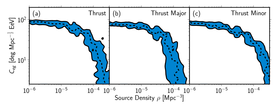
Figure 4: Expected exclusion limits on the deflection strength in the extragalactic magnetic field $C_{eg}$ for $\sim$20\,000\text{\,}$$ observed UHECR protons (dashed line) as a function of the source density. The blue shaded area denotes the limits for a $\pm 1\sigma$ fluctuation of the observed likelihood ratio $Q_{obs}$ in equation 5.

In figure 4 the expected limits on the deflection strength $C_{eg}$ in the extragalactic magnetic field as a function of the density of point sources in the simulations is shown for $\sim$20\,000\text{\,}$$ detected UHECR protons above $5\text{\,}\mathrm{EeV}$. In the simulations, deflections expected from a JF2012 [15] regular field and a limited field of view of a typical earth-bound observatory are included [22]. To account for the non-uniform exposure, the energies of the individual UHECR in eq. 1 are weighted by the relative exposure in the arrival direction. By measuring the thrust observables using a current UHECR experiment, scenarios can be tested, in which UHECR are protons that originate from point sources with a density less than $\rho\approx$1\text{\times}{10}^{-5}\text{\,}{\mathrm{Mpc}}^{-3}$$ and exhibit deflections weaker than $C_{eg}\approx$90\text{\,}\mathrm{\SIUnitSymbolDegree}\text{\,}{\mathrm{Mpc}}^{-1/2}\text{\,}\mathrm{EeV}$$ in the extragalactic magnetic field.

5 Conclusion

We presented a method to characterize the directional energy distribution of UHECR using the thrust observables from high energy physics. The directions of preferred deflection are identified as directions of the principal axes with this method. The distribution of thrust observables measured in localized region in the sky can be used to compare observations with predictions from model scenarios. For UHECR being protons, we estimated that with the statistic of current UHECR experiments, scenarios with deflections up to $C_{eg}\approx$90\text{\,}\mathrm{\SIUnitSymbolDegree}\text{\,}{\mathrm{Mpc}}^{-1/2}\text{\,}\mathrm{EeV}$$ can be tested, if the density of sources is compatible with the density of radio loud AGN.

Acknowledgment:  This work is supported by the Ministerium für Wissenschaft und Forschung, Nordrhein-Westfalen, and the Bundesministerium für Bildung und Forschung (BMBF). T. Winchen gratefully acknowledges funding by the Friedrich-Ebert-Stiftung.

References

- [1] M. S. Sutherland, B. M. Baughman, J. J. Beatty, Astroparticle Physics 34, 198 (2010).
- [2] R. Aloisio, D. Boncioli, A. Grillo, S. Petrera, F. Salamida, JCAP 1210, 007 (2012).
- [3] K.-H. Kampert, et al., Astroparticle Physics 42, 41 (2013).
- [4] H.-P. Bretz, M. Erdmann, P. Schiffer, D. Walz, T. Winchen, arXiv:1302.3761, submitted to Astroparticle Physics (2013).
- [5] M. De Domenico, arXiv:1305.4364 (2013).
- [6] J. Abraham, et al., Nuclear Instruments and Methods A613, 29 (2010).
- [7] J. Abraham, et al., Nuclear Instruments and Methods 620, 227 (2010).
- [8] T. Abu-Zayyad, et al., Nuclear Instruments and Methods A689, 87 (2012).
- [9] H. Tokuno, et al., Nuclear Instruments and Methods A676, 54 (2012).
- [10] S. Lee, A. V. Olinto, G. Sigl, Astrophysical Journal 455, L21–L24 (1995).
- [11] P. Abreu, et al., Astroparticle Physics 35, 354 (2012).
- [12] P. Abreu, et al., JCAP (in press), arXiv:1305.1576 (2013).
- [13] S. Brandt, C. Peyrou, R. Sosnowski, A. Wroblewski, Physics Letters 12, 57 (1964).
- [14] T. Winchen, Ph.D. thesis, RWTH Aachen University (Submitted in April 2013).
- [15] R. Jansson, G. R. Farrar, Astrophysical Journal 757, 14 (2012).
- [16] A. L. Read, Proceedings of the 1st Workshop on Confidence Limits, 81, (CERN, Geneva, 2000).
- [17] A. L. Read, Journal of Physics G 28, 2693 (2002).
- [18] R. Barate, et al., Physics Letters B 565, 61 (2003).
- [19] T. Aaltonen, et al., Physical Review Letters 104, 061802 (2010).
- [20] G. Aad, et al., Physical Review D 86, 032003 (2012).
- [21] S. Chatrchyan, et al., Physics Letters B 710, 26 (2012).
- [22] P. Sommers, Astroparticle Physics 14, 271 (2001).