Disordered Josephson junction chains: Anderson localization of normal modes and impedance fluctuations

Abstract

We study the properties of the normal modes of a chain of Josephson junctions in the simultaneous presence of disorder and absorption. We consider the superconducting regime of small phase fluctuations and focus on the case where the effects of disorder and absorption can be treated additively. We analyze the frequency shift and the localization length of the modes. We also calculate the distribution of the frequency-dependent impedance of the chain. The distribution is Gaussian if the localization length is long compared to the absorption length; it has a power law tail in the opposite limit.

I Introduction

For more than a decade now, one-dimensional chains of Josephson junctions have been used as controlled electromagnetic environments in experiments on superconducting nanocircuits. This includes their use as high-impedance environments Watanabe2001 ; Corlevi2006a ; Corlevi2006b , and more recently as superinductors Manucharyan2009 ; Masluk2012 ; Bell2012 . Indeed, depending on the ratio of the characteristic charging energy $E_{C}$ and Josephson coupling energy $E_{J}$, Josephson junction chains can be tuned into the insulating regime, $E_{C}/E_{J}\gg 1$, characterized by a highly resistive response, or the superconducting regime, $E_{C}/E_{J}<1$, with a response dominated by the total effective Josephson inductance Bradley1984 ; Chow1998 ; Haviland2000 ; Kuo2001 ; Miyazaki2002 ; Takahide2006 ; Fazio2001 . The use of chains made out of SQUID loops makes it possible to tune the ratio $E_{C}/E_{J}$ in situ experimentally by varying the applied magnetic flux Haviland2000 .

In the superconducting regime, the fluctuations of the superconducting phase difference across each junction in the chain are small Fazio2001 . The chain behaves as an effective LC transmission line, sustaining propagating electromagnetic modes. Details of the chain’s electromagnetic response depend on the properties of these modes. In this paper we focus on the superconducting regime and consider disordered chains, for which the values of the parameters of the junctions forming the chain vary randomly from one junction to the other. Dyson Dyson1953 was the first to analyze the frequency distribution of the normal modes of disordered LC transmission lines. Later, the spectral properties of random chains were investigated in the framework of localization phenomena Ziman1982 . These studies neglected effects related to absorption. Absorption should be taken into account in the case of Josephson junction chains, as Josephson junctions are generally characterized by a finite quality factor Likharev1986 ; Schoen1990 . Effects of absorption and disorder have been studied in Refs. Freilikher1994, ; PradhanKumar, ; BruceChalker, ; Beenakker1996, ; Misirpashaev1996, ; Deych2001, for the one-dimensional Helmholtz equation with spatially fluctuating dielectric constant.

In this paper, we analyze the effects of the simultaneous presence of disorder and absorption on the electromagnetic properties of Josephson junction chains in the superconducting regime. Here we consider the whole range of frequencies, and only in the low-frequency limit can the Josephson junction chain be effectively described by the Helmholtz equation. Specifically, we study the properties of the normal modes and calculate the localization length and frequency shift for the case where absorption and disorder act additively. We also study the statistics of the chain’s frequency-dependent impedance and calculate its distribution. The corresponding main results of the paper are represented by Eqs. (13), (14), (21), and (22).

Our results are relevant in view of the aforementioned experiments, in which uniform Josephson junction chains are implemented as tunable environments in quantum circuitryWatanabe2001 ; Corlevi2006a ; Corlevi2006b ; Manucharyan2009 ; Masluk2012 ; Bell2012 . Disorder is inevitably present when fabricating Josephson junction arrays and knowledge as to what disorder levels are acceptable in order for the chains to be uniform enough for applications is important. On the other hand, our results can also be useful in the context of mode engineering. Indeed, using intentionally induced disorder, certain modes will be localized, thus suppressing the electromagnetic response of the chain at the corresponding frequencies, which might be of interest for applications of chains as electromagnetic environments.

The paper is organized as follows. We start by exposing the model in Section II and present a qualitative discussion of the main results in Section III. The detailed calculations are presented in Sections IV – VI. Determining the normal modes for a disordered Josephson junction chain in the presence of absorption corresponds to solving a non-Hermitian eigenvalue problem which we address in section IV. The localization length of the normal modes is calculated in Section V. The statistics of the chain’s impedance is analyzed in Section VI; Section VII contains our conclusions.

II The model

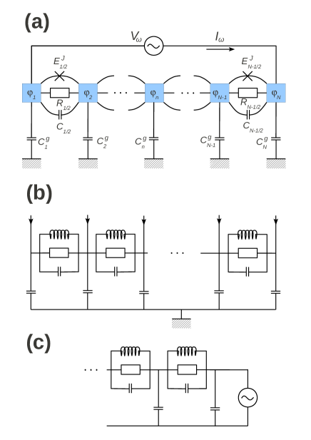
Figure 1: (color online) (a) A schematic view of the Josephson junction chain and its impedance measurement. (b) The transmission line described by Eqs. (2), equivalent to the chain shown in (a) for $I_{N}=-I_{1}=I_{\omega}$, $I_{2},\ldots,I_{N-1}=0$, $V_{N}-V_{1}=V_{\omega}$. (c) The circuit used to define the impedance of a semi-infinite chain.

The chain to be studied in the present paper is assumed to consist of $N$ superconducting islands, labelled by an integer $n=1,\ldots,N$. The Josephson junction between the islands $n$ and $n+1$ is labelled by the half-integer $n+1/2$. We focus on small oscillations of the superconducting phase $\theta_{n}$ of each island, so that the Josephson current through the $(n+1/2)$th junction, $I^{c}_{n+1/2}\sin(\theta_{n+1}-\theta_{n})$, can be linearized as $I^{c}_{n+1/2}(\theta_{n+1}-\theta_{n})$ here $I^{c}_{n+1/2}$ is the critical current of the junction, related to the Josephson energy $E^{J}_{n+1/2}=\hbar{}I^{c}_{n+1/2}/(2e)$]. The observable quantity on which we focus in the present paper is the complex impedance $Z(\omega)$ of the chain at the frequency $\omega$, defined as the ratio of the voltage $V_{\omega}$ on an external ac voltage source, connected to the first and the last islands of the chain, to the current $I_{\omega}$ through this source, as shown in Fig. 1(a). The complex impedance is in one-to-one correspondence with the reflection coefficient of the equivalent transmission line, shown in Fig. 1(b), as discussed in Appendix A.

For small oscillations, the superconducting phases of the chain of $N$ islands at frequency $\omega$ can be represented as

$$\theta_{n}(t)=\theta_{n}(0)+\frac{2eV_{n}}{\hbar}\,\frac{e^{-i\omega{t}}}{-i\omega},$$ (1)

where $V_{n}$ is the ac voltage on the $n$th island, and $e<0$ is the electron charge. The voltages satisfy the following system of linear equations:

$$\begin{split}&Y_{3/2}(V_{1}-V_{2})-i\omega{C}^{g}_{1}V_{1}=I_{1},\\ &Y_{n-1/2}(V_{n}-V_{n-1})+Y_{n+1/2}(V_{n}-V_{n+1})-i\omega{C}_{n}^{g}V_{n}=I_{n}\quad(1<n<N),\\ &Y_{N-1/2}(V_{N}-V_{N-1})-i\omega{C}^{g}_{N}V_{N}=I_{N}.\end{split}$$ (2)

The $n$th equation of this system is nothing but the first Kirchhoff law (current conservation condition) at the $n$th island. $I_{n}$ represents an external current injected into the $n$th island (actually, the setting shown in Fig. 1(a) corresponds to only $I_{N}=-I_{1}$ being non-zero, but we include all $I_{n}$’s to formally display the right-hand side of the linear system). Each island is assumed to have some capacitance $C_{n}^{g}$ with respect to the ground, so $-i\omega{C}_{n}^{g}V_{n}$ is the displacement current leaking to the ground through this capacitance. $Y_{n+1/2}$ is the admittance of the $(n+1/2)$th junction, so $Y_{n+1/2}(V_{n}-V_{n+1})$ is the current leaving the $n$th island through this junction. In accordance with the standard RCSJ-model for Josephson junctions Likharev1986 ; Schoen1990 , the admittance includes three terms:

$$Y_{n+1/2}(\omega)=-\frac{1}{i\omega{L}_{n+1/2}}-i\omega{C}_{n+1/2}+\frac{1}{R_{n+1/2}}.$$ (3)

The first one represents the linearized Josephson contribution $I^{c}_{n+1/2}(\theta_{n+1}-\theta_{n})$, by virtue of Eq. (1) and by the definition of the Josephson inductance $L_{n+1/2}=-\hbar/(2eI^{c}_{n+1/2})$. The second term is the contribution of the capacitive electrostatic coupling between the neighboring islands. Finally, $1/R_{n+1/2}$ is the dissipative junction conductance due to the normal current carried by quasiparticles. It is expected to vanish ($R_{n+1/2}\to\infty$) at zero temperature, and approach the normal state conductance as the critical temperature is approached. The system (2) corresponds to the effective electric circuit shown in Fig. 1(b).

For a weakly disordered Josephson junction chain, the capacitances, inductances and resistances of its elements can be represented as

$$\begin{split}&C^{g}_{n}=C^{g}(1+\eta_{n}),\\ &L_{n+1/2}=\frac{L}{1+\zeta_{n}},\\ &C_{n+1/2}=C(1+\zeta_{n}),\end{split}$$ (4)

where the weak relative fluctuations $\eta_{n},\zeta_{n}$ are independent Gaussian random variables with zero average and

$$\langle\eta_{n}^{2}\rangle=\sigma_{g}^{2},\quad\langle\zeta_{n}^{2}\rangle=\sigma_{S}^{2}.$$ (5)

Here the angular brackets denote the statistical average, and variables with different $n$’s are uncorrelated. The assumption of weak disorder implies $\sigma_{g},\sigma_{S}\ll{1}$. Note that the fluctuations of $L_{n+1/2}$ and $C_{n+1/2}$ are not independent: the product $L_{n+1/2}C_{n+1/2}\equiv 1/\omega_{p}^{2}$ is assumed to be constant, equal to the inverse squared junction plasma frequency $\omega_{p}$. This is because we assume that the fluctuations of $L$ and $C$ are due to fluctuations of the junction sizes $S$. Typically, $L\sim 1/S$, whereas $C\sim S$.

We do not consider the fluctuations of the normal resistances, assuming $R_{n+1/2}=R$. We are interested in the regime of large $R$, when the average effect of the resistance (namely, the absorption) is small; weak fluctuations of $R$ acting on top of this small average have a negligible effect on the statistics of impedance, as compared to the fluctuations of inductances and capacitances. This can be checked directly by repeating the calculations of Sec. VI in the presence of fluctuations of $R$; they are fully analogous but more cumbersome, and the result is quite trivial. Thus, we prefer to neglect the fluctuations of $R$ from the very beginning.

III Qualitative discussion and summary of the main results

We start by noting that the system (2) can be used to study two, generally speaking, physically distinct problems.

The first one is the problem of free oscillations (eigenmodes), which consists in finding nontrivial solutions for the voltages $V_{n}$ when all external currents $I_{n}=0$. Such solutions exist only for some special values of $\omega$, which are, generally speaking, complex, because of the dissipation induced by the resistors. Physically, these solutions represent charge distributions which oscillate and relax exponentially in time while maintaining their spatial shape (which corresponds to a gedanken experiment, rather than a real one). Mathematically, this corresponds to a non-Hermitian quadratic eigenvalue problem, to be discussed in detail in Sec. IV. In an infinite disorder-free chain the solutions are necessarily plane waves, $V_{n}\propto{e}^{ikn}$, so the corresponding frequencies define the dispersion relation $\Omega(k)$ which is a complex function of a real argument $k$. This dispersion relation can be represented as a curve in the complex plane of $\omega$ (Fig. 2). In a disordered system, the eigenmodes are no longer plane waves, but are exponentially localized with some localization length $\xi$. Strictly speaking, their frequencies do not form a continuous curve in the complex plane of $\omega$, but rather represent a set of points. Still, when the disorder is weak, so that the localization length $\xi$ is sufficiently large, the uncertainty in the wave vector $1/\xi\ll{k}$, so the points lie in the vicinity of the original dispersion curve of the disorder-free chain (Fig. 2). To the leading order in the disorder strength, one can speak about the localization length $\xi$ as a function of the wave vector $k$.

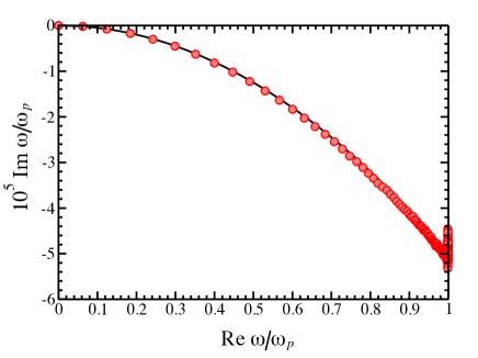
Figure 2: Complex plane of $\omega$ in the units of $\omega_{p}\equiv(LC)^{-1/2}$. The solid line shows the dispersion curve $\Omega(k)$ for $\omega_{p}RC=10^{4}$, $C^{g}/C=0.01$. The symbols represent the frequencies of the normal modes of a disordered chain with $N=500$ islands and $\sigma_{S}^{2}=0.1$, $\sigma_{g}^{2}=0$. The condition $\xi(\omega)<N$ is fulfilled only for $\omega/\omega_{p}>0.969\ldots$, so most of the interval $0<\omega<\omega_{p}$ is occupied by modes which are weakly perturbed by the disorder. However, most of the modes (about 87%) lie in the narrow frequency interval with $\xi(\omega)<N$. Strong fluctuations of $\mathop{\mathrm{Im}}\nolimits\omega$, seen as the vertical feature on the right edge of the figure, occur for the modes whose frequencies lie close to the band edge of the clean chain. Their localization lengh is $\xi\sim{1}$, so the approach used in the present paper is not valid for their description.

The second problem is that of forced oscillations, which consists in finding the voltage profile $V_{n}$ in the presence of external currents $I_{n}$, oscillating at a real frequency $\omega$. In particular, the impedance of the chain $Z(\omega)$, introduced in the beginning of the previous section (Fig. 1), is found from the solution of such a problem with the currents applied to the two ends of the chain, while away from the ends $I_{2}=\ldots=I_{N-1}=0$. Mathematically, the problem is just to invert the matrix of the system (2). In the absence of disorder, the voltage profile away from the ends is still represented by plane waves. However, in the presence of dissipation, the corresponding wave vector must be complex: $V_{n}\propto{e}^{i(k+i\kappa)n}$, and $k+i\kappa$ are determined by the solutions of the equation $\Omega(k+i\kappa)=\omega$ with real $\omega$. Physically, this means that the ac excitation penetrates the chain only within the distance $\sim{1}/\kappa$ from the ends, and at longer distances it decays because of the absorption. Thus, $1/\kappa$ can be called the absorption length. In a disordered chain, the solution for $V_{n}$ decays away from the ends even in the absence of dissipation, due to the localization, and the corresponding length scale is the localization length $\xi$.

When both dissipation and disorder are present, they both contribute to the spatial decay of the solution (whose rate is called Lyapunov exponent), and, generally speaking, their effects are not easy to separate. For this reason, the notion of the localization length as a function of frequency in the complex plane is not very well defined in the presence of dissipation. Still, in the limit of weak disorder and weak dissipation the effects of localization and absorption can be assumed to be additive. Namely, the Lyapunov exponent is given by the sum $\kappa+1/\xi$ where $\kappa$ is calculated for weak dissipation and no disorder (that is, small $1/R$ and $\sigma_{g}^{2},\sigma_{S}^{2}=0$) while $\xi$ is calculated for weak disorder and no dissipation (that is, $1/R=0$ and small $\sigma_{g}^{2},\sigma_{S}^{2}$). Indeed, the additive expression $\kappa+1/\xi$ is nothing but the first (linear) term in the expansion of the Lyapunov exponent in the small parameters $1/R,\sigma_{g}^{2},\sigma_{S}^{2}$. If this first term is not sufficient, localization and dissipation cannot be assumed to enter additively.

For the particular case of the chain, shown in Fig. 1 and described by Eqs. (2), the dispersion relation of the disorder-free chain is well-known in the absence of dissipation ($R\to\infty$),Fazio2001 ; Rastelli2012 ; Masluk2012 and can be straightforwardly generalized to the case of finite $R$:

$$\frac{\Omega(k)}{\omega_{p}}=\sqrt{\frac{2\epsilon_{k}}{2\epsilon_{k}+\ell^{-2}}-\frac{\epsilon_{k}^{2}/Q^{2}}{(2\epsilon_{k}+\ell^{-2})^{2}}}-i\,\frac{\epsilon_{k}/Q}{2\epsilon_{k}+\ell^{-2}},$$ (6)

where we have denoted

$$\epsilon_{k}\equiv{2}\sin^{2}\frac{k}{2},\;\;\;\omega_{p}\equiv\frac{1}{\sqrt{LC}},\;\;\;\ell^{-2}\equiv\frac{C^{g}}{C},\;\;\;Q\equiv\omega_{p}{RC}.$$ (7)

Here $\omega_{p}$ is the plasma frequency of a single junction, which is a convenient unit of frequency, $Q$ is the quality factor of a single junction, which is nothing but the resistance $R$ in the units of $\sqrt{L/C}$, and $\ell$ is the screening length, so that $\ell^{-2}$ is the ground capacitance $C^{g}$ in the units of $C$. The real wave vector $k$ varies from 0 to $\pi$ for an infinite chain, while for a chain of $N$ islands assumes $N$ discrete values,

$$k=0,\frac{\pi}{N},\frac{2\pi}{N},\ldots,\frac{(N-1)\pi}{N},$$ (8)

the eigenmodes of the system being $V_{n}\propto\cos{k}(n-1/2)$. For the low-frequency modes at small $k\ll\min\{1,\ell^{-1}\}$,

$$\frac{\mathop{\mathrm{Re}}\nolimits\Omega(k)}{\omega_{p}}\approx{k}\ell,\quad\frac{\mathop{\mathrm{Im}}\nolimits\Omega(k)}{\omega_{p}}\approx-\frac{(k\ell)^{2}}{2Q},$$ (9)

so that their damping is weak, $|\mathop{\mathrm{Im}}\nolimits\Omega(k)|\ll|\mathop{\mathrm{Re}}\nolimits\Omega(k)|$, even if the quality factor is not very high.

The inverse absorption length $\kappa$ for the disorder-free chain at real $\omega$ should be found as the solution of the equation $\Omega(k+i\kappa)=\omega$, which is equivalent to

$$1-\cos(k+i\kappa)=\frac{\varpi^{2}\ell^{-2}/2}{1-\varpi^{2}-i\varpi/Q},\quad\varpi\equiv\frac{\omega}{\omega_{p}}.$$ (10)

The resulting expression for $\kappa$ is rather lengthy, so we give here the approximate expression, valid to the leading order in $1/Q\ll{1}$:

$$\kappa=\frac{1}{Q}\,\frac{\varpi^{2}\ell^{-1}/2}{(1-\varpi^{2})\sqrt{1-\varpi^{2}-\varpi^{2}\ell^{-2}/4}}+O(Q^{-2}).$$ (11)

Note that to the leading order in $Q^{-1}$, we have $\kappa=-\mathop{\mathrm{Im}}\nolimits\Omega(k)/(d\mathop{\mathrm{Re}}\nolimits\Omega(k)/dk)$, which corresponds to the solution of $\Omega(k+i\kappa)=\omega$ perturbatively in the imaginary parts.

The impedance of a finite disorder-free chain [as defined in Fig. 1(a)] can be represented as a sum over the eigenmodes (see Sec. IV for details):

$$Z(\omega)=\sum_{k}\left[\frac{iA_{k}}{\omega-\Omega(k)}+\frac{iA_{k}^{*}}{\omega+\Omega^{*}(k)}\right],$$ (12a)

$$A_{k}=\frac{1}{N}\,\frac{4\cos^{2}(k/2)\sin^{2}(kN/2)}{C^{g}+\epsilon_{k}[2C+i/\Omega(k)R]}.$$ (12b)

For a disordered chain, we have calculated the localization length $\xi$ in the limit of weak disorder and no dissipation (see Sec. V for details). As discussed in the beginning of this section, to the leading order in the disorder strength, one can still label the eigenstates by their wave vector $k$, and speak about the $k$-dependent localization length, which is given by

$$\frac{1}{\xi}=\frac{\sigma_{S}^{2}+\sigma_{g}^{2}}{2}\,\tan^{2}\frac{k}{2}=\frac{\left(\sigma_{S}^{2}+\sigma_{g}^{2}\right)\varpi^{2}\ell^{-2}/8}{1-\varpi^{2}-\varpi^{2}\ell^{-2}/4}.$$ (13)

Since $\sigma_{R}^{2},\sigma_{g}^{2}\ll{1}$, the inequality $1/\xi\ll{k}$ holds almost everywhere, except for a narrow region of $k$ around $k=\pi$. At $\omega\to{0}$ the localization length diverges as $1/\omega^{2}$. Such low-frequency behaviour is quite common for disordered bosonic problems.Ziman1982 ; John1983 ; Gurarie2003 ; Bilas2006 In our case, the divergence is related to the existence of the delocalized zero mode, i.e., an eigenmode with $\omega=0$, $V_{n}=\mathrm{const}$, when no currents flow in the system, for any realization of the disorder. This is the Goldstone mode related to the global gauge invariance of the system.

The case of short chains, $N\ll\xi,1/\kappa$, is the simplest to analyze theoretically, and at the same time it is quite relevant for experiments. Due to the condition $N\ll{1}/\kappa$, the spacing between eigenmode frequencies is larger than their broadening, so the discrete modes are well resolved. The condition $N\ll\xi$ ensures that corrections to the eigenmode profiles and frequencies are relatively small. The latter, however, does not mean that the correction to the impedance of the chain is small. Indeed, the impedance changes significantly when the eigenmode frequency shift $\delta\omega_{k}$ due to disorder is of the order of the broadening $\mathop{\mathrm{Im}}\nolimits\Omega(k)$, even if $\delta\omega_{k}$ is small compared to the frequency $\mathop{\mathrm{Re}}\nolimits\Omega(k)$ itself. At the same time, the disorder-induced corrections to the amplitude $A_{k}$ and to the broadening produce just small corrections to the impedance. Thus, we focus on the random shift $\delta\omega_{k}$, calculated perturbatively in Sec. IV. The average $\langle\delta\omega_{k}\rangle=0$, and the fluctuations are given by

$$\frac{\langle\delta\omega_{k}^{2}\rangle}{\omega_{p}^{2}}=\frac{3}{8}\,\frac{\sigma_{S}^{2}+\sigma_{g}^{2}}{N}\,\frac{2\epsilon_{k}\,\ell^{-4}}{(2\epsilon_{k}+\ell^{-2})^{3}}.$$ (14)

When the chain is long compared to the inverse Lyapunov exponent, $N\gg(\kappa+1/\xi)^{-1}$, the two ends of the chain are effectively decoupled. Then the impedance of the chain $Z(\omega)$, as defined in Fig. 1(a), equals to the sum of the impedances of two semi-infinite chains, shown in Fig. 1(c). The impedance of a semi-infinite chain in the absence of disorder, which we denote by $Z_{\infty}^{(\mathrm{c})}(\omega)$, is given by

$$\begin{split}&Z_{\infty}^{(\mathrm{c})}(\omega)=\frac{1}{2Y(\omega)}\left(-1+\sqrt{1-\frac{4Y(\omega)}{i\omega{C}^{g}}}\right),\\ &Y(\omega)\equiv-\frac{1}{i\omega{L}}+\frac{1}{R}-i\omega{C}.\end{split}$$ (15)

When disorder is present, the two ends of a sufficiently long chain feel two different realizations of disorder, so $Z(\omega)$ is a sum of two impedances $Z_{\infty}(\omega)$, which are statistically independent. Thus, to characterize the statistics of $Z(\omega)$, it is sufficient to find the statistics of the impedance $Z_{\infty}(\omega)$ of a semi-infinite chain. This impedance is given by the lower right (i.e., $N,N$) element of the inverse matrix of the system (2). So far we have made the assumptions of weak dissipation, which implies $k\gg\kappa$, and of weak disorder, $k\gg{1}/\xi$. Still, under these assumptions, two possible regimes can be identified: $\kappa\gg{1}/\xi$ and $\kappa\ll{1}/\xi$. The difference in statistics of the impedance in the two regimes can be understood from the following qualitative arguments.

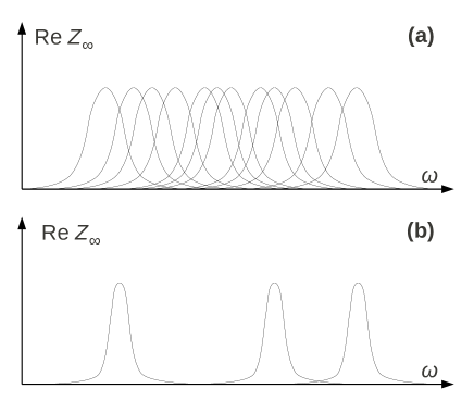
Figure 3: A schematic representation of different terms contributing to $\mathop{\mathrm{Re}}\nolimits{Z}_{\infty}$ (a) at $\delta_{\xi}\ll\gamma$ (strongly overlapping Lorentzians), and (b) at $\delta_{\xi}\gg\gamma$ (well-separated Lorentzians).

Let us focus on the real part of the impedance, which determines the absorption. In terms of the complex eigenmode frequencies which we write as $\Omega_{\alpha}=\pm\omega_{\alpha}-i\gamma_{\alpha}$, $\alpha=1,\ldots,N-1$, absorption can be represented by a sum of Lorentzians corresponding to the eigenmodes:

$$\mathop{\mathrm{Re}}\nolimits{Z}_{\infty}(\omega)=\sum_{\alpha,\pm}\frac{\gamma_{\alpha}{A}_{\alpha}}{(\omega\pm\omega_{\alpha})^{2}+\gamma_{\alpha}^{2}}$$ (16)

(the imaginary parts of $A_{\alpha}$ have been neglected). Even though the number of terms in the sum can be very large, only those modes effectively contribute to the sum, which are located within a distance $\sim\xi$ from the end; for others, the coefficient $A_{\alpha}$ is exponentially small. The typical distance between the Lorentzians corresponds to the typical frequency spacing $\delta_{\xi}$ between the modes within one localization length $\xi$, while the typical width of each Lorentzian is $\gamma$. Clearly, one can imagine two regimes, depending on the relation between $\gamma$ and $\delta_{\xi}$. When $\delta_{\xi}\ll\gamma$, the Lorentzians overlap strongly, so the fluctuations of $Z_{\infty}(\omega)$ are much smaller than its average [Fig. 3(a)]. When $\delta_{\xi}\gg\gamma$, the Lorentzians are well separated, and, depending on the realization of the disorder, the frequency $\omega$ may either fall near one of the peak centers $\omega_{\alpha}$, which gives a large absorption, or it may fall between the peaks, and then the absorption will be small [Fig. 3(b)]. Thus, in the case $\delta_{\xi}\gg\gamma$, the fluctuation will be strong, so the disorder-averaged impedance is not a very useful concept; rather, the whole distribution function can be evaluated. Finally, we recall the relation $\kappa=\gamma/[d\mathop{\mathrm{Re}}\nolimits\Omega(k)/dk]$, established earlier, and note that the density of modes within the localization length can also be evaluated using the disorder-free dispersion, $1/\delta_{\xi}=\xi\,dk/[2\pi\,d\!\mathop{\mathrm{Re}}\nolimits\Omega(k)]$. Thus, the parameter controlling the two regimes is precisely

$$\frac{\gamma}{\delta_{\xi}}=\frac{\kappa\xi}{2\pi},$$ (17)

and the mode group velocity $d\mathop{\mathrm{Re}}\nolimits\Omega(k)/dk$ drops out.

Based on this picture, one can make some estimates. Let us assume that the main source of fluctuations of $Z_{\infty}(\omega)$ are the random positions $\omega_{\alpha}$. Let us choose an interval of frequencies, centered at $\omega$ and having the width $\Delta$, such that $\delta_{\xi},\gamma\ll\Delta\ll\omega$. Let us count only those modes whose frequencies $\omega_{\alpha}$ fall inside this interval; indeed, the modes whose positions $\omega_{\alpha}$ are too far from $\omega$ (further than a few times $\gamma$), contribute very little to the sum in Eq. (16). Typically, there are $N_{\xi}=\Delta/\delta_{\xi}$ modes inside the interval. For all such modes, let us set all $\gamma_{\alpha}$’s equal to a constant $\gamma$, and all $A_{\alpha}=A$ (the smooth dependence of $A$ and $\gamma$ on $\omega$ can be neglected due to the condition $\Delta\ll\omega$). As for the peak positions $\omega_{\alpha}$, let us assume them to be uniformly and independently distributed over the interval $(\omega-\Delta/2,\omega+\Delta/2)$. Of course, such a Poisson distribution totally neglects level repulsion, but for our quantitative estimate is good enough. The average $\mathop{\mathrm{Re}}\nolimits{Z}_{\infty}$ is then given by

$$\begin{split}\langle\mathop{\mathrm{Re}}\nolimits{Z}_{\infty}\rangle={}&{}\int\limits_{\omega-\Delta/2}^{\omega+\Delta/2}\frac{d\omega_{1}}{\Delta}\ldots\frac{d\omega_{N_{\xi}}}{\Delta}\sum_{\alpha=1}^{N_{\xi}}\frac{\gamma{A}}{(\omega-\omega_{\alpha})^{2}+\gamma^{2}}=\\ ={}&{}\frac{N_{\xi}}{\Delta}\,\pi{A}=\frac{\pi{A}}{\delta_{\xi}}.\end{split}$$ (18)

Let us now study the probability distribution of the dimensionless impedance, relative to its average value, which we denote by $x$:

$$\begin{split}P(x)={}&{}\int\limits_{\omega-\Delta/2}^{\omega+\Delta/2}\frac{d\omega_{1}}{\Delta}\ldots\frac{d\omega_{N_{\xi}}}{\Delta}\times\\ {}&{}\times\delta\!\left(x-\sum_{\alpha=1}^{N_{\xi}}\frac{\delta_{\xi}\gamma/\pi}{(\omega-\omega_{\alpha})^{2}+\gamma^{2}}\right).\end{split}$$ (19)

This probability distribution can be straightforwardly evaluated in the two limiting cases $\delta_{\xi}\ll\gamma$ and $\delta_{\xi}\gg\gamma$ (see Appendix B for details).

For $$\delta_{\xi}\ll\gamma$$, we have

$$P(x)=\sqrt{\gamma/\delta_{\xi}}\,e^{-(\pi\gamma/\delta_{\xi})(x-1)^{2}}.$$ (20a)

The narrow Gaussian distribution arises naturally as a consequence of the central limit theorem, since there are many terms in the sum (16) which contribute to $$\mathop{\mathrm{Re}}\nolimits{Z}_{\infty} \delta_{\xi}\gg\gamma$$. For ,

$$P(x)=\frac{e^{-\gamma/(x\delta_{\xi})}}{\pi{x}^{3/2}\sqrt{\delta_{\xi}/(\pi\gamma)-x}},\quad 0<x<\frac{\delta_{\xi}}{\pi\gamma},$$ (20b)

and $$P(x)=0$$ outside the indicated interval.

The exponential suppression of $P(x)$ at small $x$ comes from the fact that an anomalously small $x$ requires a region of frequencies of the width $\Delta\omega\gg\delta_{\xi}$, free of Lorentzians. For the Poisson distribution of $\omega_{\alpha}$’s, assumed here, the probability to have such a region vanishes as $e^{-\Delta\omega/\delta_{\xi}}$; if level repulsion is taken into account, the supression is even stronger. The weak singularity at large $x=\delta_{\xi}/(\pi\gamma)$ is a consequence of the assumption $A_{\alpha}=A$, $\gamma_{\alpha}=\gamma$, which implies that all Lorentzians have the same height. In reality, a spread in the heights smears the singularity.

In Sec. VI, we calculate the distribution function of $Z_{\infty}$ in the regime of weak fluctutations ($\kappa\xi\gg{1}$) using the Fokker-Planck equation:

$$P(Z_{\infty})\propto\exp\left(-\frac{\kappa\xi}{4}\,\frac{|Z_{\infty}-Z_{\infty}^{(\mathrm{c})}|^{2}}{|Z_{\infty}^{(\mathrm{c})}|^{2}}\right),$$ (21)

where $\kappa$, $\xi$, and $Z_{\infty}^{(\mathrm{c})}(\omega)$ are given by Eqs. (11), (13), and (LABEL:Zc=), respectively. Keeping in mind the relation (17), we see that the semi-qualitative Eq. (75a) gives the correct functional form (Gaussian), underestimating the fluctuations by a factor of 2. The latter is not surprising, as in deriving Eq. (75a) we completely ignored the fluctuations of the eigenmode amplitudes and widths. Eq. (21) has also been confirmed by direct numerical sampling.Crisan

In the regime of strong fluctuations, $\kappa\xi\ll{1}$, we were unable to solve the problem analytically, so we analyzed it numerically (see Sec. VI). Our numerical results, indeed, indicate that the distribution of $\mathop{\mathrm{Re}}\nolimits{Z}_{\infty}$ has a power-law tail described by

$$P(\mathop{\mathrm{Re}}\nolimits{Z}_{\infty})\approx C\,\frac{(\kappa\xi)^{0.5}}{\mathop{\mathrm{Re}}\nolimits{Z}_{\infty}^{(\mathrm{c})}}\left(\frac{\mathop{\mathrm{Re}}\nolimits{Z}_{\infty}^{(\mathrm{c})}}{\mathop{\mathrm{Re}}\nolimits{Z}_{\infty}}\right)^{1.5},\quad C\sim 0.3-0.5,$$ (22)

in agreement with Eq. (20b). This also agrees with the distribution of the reflection coefficient, calculated for the one-dimensional Helmholtz equation with spatially fluctuating dielectric constant in Ref. PradhanKumar, (see Appendix A for the relation between the impedance and the reflection coefficient).

IV The eigenvalue problem

To begin with, we note that the formal manipulations performed in this section, in fact, are quite analogous to those for the elementary damped harmonic oscillator. The latter is discussed in Appendix C in order to make the present section more transparent.

Let us write the system (2) in a compact form:

$$\left(\hat{L}^{-1}-i\omega\hat{R}^{-1}-\omega^{2}\hat{C}\right){\rm\bf V}=-i\omega{\rm\bf I},$$ (23)

where ${\rm\bf V}$ and ${\rm\bf I}$ are $N$-dimensional column vectors containing the node voltages $V_{n}$ and currents $I_{n}$, respectively, and $\hat{L}^{-1}$, $\hat{R}^{-1}$, and $\hat{C}$ are real, symmetric, tridiagonal matrices. Besides, they are positive-definite; indeed, for an arbitrary real vector ${\rm\bf x}$,

$${\rm\bf x}^{T}\hat{L}^{-1}{\rm\bf x}=\sum_{n=1}^{N-1}\frac{(x_{n+1}-x_{n})^{2}}{L_{n+1/2}}\geq{0},$$ (24a)

$${\rm\bf x}^{T}\hat{R}^{-1}{\rm\bf x}=\sum_{n=1}^{N-1}\frac{(x_{n+1}-x_{n})^{2}}{R_{n+1/2}}\geq{0},$$ (24b)

$${\rm\bf x}^{T}\hat{C}{\rm\bf x}=\sum_{n=1}^{N-1}C_{n+1/2}(x_{n+1}-x_{n})^{2}+\sum_{n=1}^{N}C^{g}_{n}x_{n}^{2}>0.$$

$\hat{L}^{-1}$ and $\hat{R}^{-1}$ have exactly one zero eigenvalue with the eigenvector ${\rm\bf x}_{0}=(1\>1\ldots{1})^{T}/\sqrt{N}$. At the same time, ${\rm\bf x}_{0}^{T}\hat{C}{\rm\bf x}_{0}=\overline{C^{g}}$, the spatial average of the ground capacitance.

Thanks to these properties, one can define the matrix square roots $\hat{L}^{-1/2},\hat{C}^{1/2}$, as well as the inverse $\hat{C}^{-1/2}$, which are also real, symmetric, and positive-definite matrices. Then the system (23), quadratic in $\omega$ can be identically rewritten as

$$\omega\mathcal{V}-\left(\begin{array}[]{cc}-i\hat{C}^{-1/2}\hat{R}^{-1}\hat{C}^{-1/2}&\hat{C}^{-1/2}\hat{L}^{-1/2}\\ \hat{L}^{-1/2}\hat{C}^{-1/2}&0\end{array}\right)\mathcal{V}=\left(\begin{array}[]{c}i\hat{C}^{-1/2}{\rm\bf I}\\ 0\end{array}\right),\quad\mathcal{V}\equiv\left(\begin{array}[]{c}\hat{C}^{1/2}{\rm\bf V}\\ {\rm\bf w}\end{array}\right)$$ (25)

where ${\rm\bf w}$ is an auxiliary $N$-dimensional column vector. It should be noted that while $\hat{L}^{-1}$, $\hat{R}^{-1}$, and $\hat{C}$ are tridiagonal and thus are relatively easy to deal with numerically, their square roots are non-local, so Eq. (25) is only convenient for formal manipulations. The main advantage of Eq. (25) is that its solutions can be expressed in terms of eigenvalues and egenvectors of the $2N\times{2}N$ matrix

$$\hat{\mathcal{A}}=\left(\begin{array}[]{cc}-i\hat{C}^{-1/2}\hat{R}^{-1}\hat{C}^{-1/2}&\hat{C}^{-1/2}\hat{L}^{-1/2}\\ \hat{L}^{-1/2}\hat{C}^{-1/2}&0\end{array}\right)$$ (26)

The matrix $\hat{\mathcal{A}}$ is non-Hermitian, so it may have less then $2N$ eigenvectors if its eigenvalues are degenerate. In a disordered system all degeneracies can be assumed to be lifted, except those which are protected by a symmetry and do not depend on the disorder realization. The only special value of $\omega$ is $\omega=0$, due to the gauge invariance, as discussed in Sec. III. For any disorder realization, it is an eigenvalue with two eigenvectors:

$$\mathcal{V}_{0\pm}=\frac{1}{\sqrt{2\overline{C^{g}}}}\left(\begin{array}[]{c}\hat{C}^{1/2}{\rm\bf x}_{0}\\ \pm{i}\sqrt{\overline{C^{g}}}{\rm\bf x}_{0}\end{array}\right).$$ (27)

Thus, with probability 1, the matrix $\hat{\mathcal{A}}$ has exactly $2N$ eigenvectors, which form a complete set. Since it is symmetric, $\hat{\mathcal{A}}^{T}=\hat{\mathcal{A}}$, different eigenvectors $\alpha$ and $\beta$ are orthogonal as

$$\mathcal{V}^{T}_{\alpha}\mathcal{V}_{\beta}={\rm\bf V}^{T}_{\alpha}\hat{C}{\rm\bf V}_{\beta}+{\rm\bf w}^{T}_{\alpha}{\rm\bf w}_{\beta}=\delta_{\alpha\beta}.$$ (28)

The matrix $\hat{\mathcal{A}}$ satisfies the property $\sigma_{z}\hat{\mathcal{A}}^{*}\sigma_{z}=-\hat{\mathcal{A}}$, where $\sigma_{z}$ is the Pauli matrix acting in the $2\times{2}$ space of $N\times{N}$ blocks. Thus, if $\omega$ is an eigenvalue of $\mathcal{A}$ with the corresponding eigenvector $(\hat{C}^{1/2}{\rm\bf V}\;{\rm\bf w})^{T}$, then $-\omega^{*}$ is also an eigenvalue, and the corresponding eigenvector is $(\hat{C}^{1/2}{\rm\bf V}^{*}\;-{\rm\bf w}^{*})^{T}$. Since the absorption is assumed to be weak, we neglect the possibility to have purely imaginary eigenvalues, and count by $\alpha=1,\ldots,N$ the eigenvalues with $\mathop{\mathrm{Re}}\nolimits\omega_{\alpha}>0$. Then the unit $2N\times{2}N$ matrix can be represented as

$$\begin{split}\hat{\openone}={}&{}\left(\begin{array}[]{cc}\hat{C}^{1/2}{\rm\bf x}_{0}{\rm\bf x}_{0}^{T}\hat{C}^{1/2}/\overline{C^{g}}&0\\ 0&{\rm\bf x}_{0}{\rm\bf x}_{0}^{T}\end{array}\right){}+{}\\ {}&{}+\sum_{\alpha=1}^{N-1}\left(\begin{array}[]{cc}\hat{C}^{1/2}{\rm\bf V}_{\alpha}{\rm\bf V}_{\alpha}^{T}\hat{C}^{1/2}&\hat{C}^{1/2}{\rm\bf V}_{\alpha}{\rm\bf w}_{\alpha}^{T}\\ {\rm\bf w}_{\alpha}{\rm\bf V}_{\alpha}^{T}\hat{C}^{1/2}&{\rm\bf w}_{\alpha}{\rm\bf w}_{\alpha}^{T}\end{array}\right){}+{}\\ &{}+{}\sum_{\alpha=1}^{N-1}\left(\begin{array}[]{cc}\hat{C}^{1/2}{\rm\bf V}_{\alpha}^{*}{\rm\bf V}_{\alpha}^{\dagger}\hat{C}^{1/2}&-\hat{C}^{1/2}{\rm\bf V}_{\alpha}^{*}{\rm\bf w}_{\alpha}^{\dagger}\\ -{\rm\bf w}_{\alpha}^{*}{\rm\bf V}_{\alpha}^{\dagger}\hat{C}^{1/2}&{\rm\bf w}_{\alpha}^{*}{\rm\bf w}_{\alpha}^{\dagger}\end{array}\right),\end{split}$$ (29)

and the resolvent of $\hat{\mathcal{A}}$ as

$$\begin{split}&(\omega-\hat{\mathcal{A}})^{-1}=\frac{1}{\omega}\left(\begin{array}[]{cc}\hat{C}^{1/2}{\rm\bf x}_{0}{\rm\bf x}_{0}^{T}\hat{C}^{1/2}/\overline{C^{g}}&0\\ 0&{\rm\bf x}_{0}{\rm\bf x}_{0}^{T}\end{array}\right){}+{}\\ &{}+{}\sum_{\alpha=1}^{N-1}\frac{1}{\omega-\omega_{\alpha}}\left(\begin{array}[]{cc}\hat{C}^{1/2}{\rm\bf V}_{\alpha}{\rm\bf V}_{\alpha}^{T}\hat{C}^{1/2}&\hat{C}^{1/2}{\rm\bf V}_{\alpha}{\rm\bf w}_{\alpha}^{T}\\ {\rm\bf w}_{\alpha}{\rm\bf V}_{\alpha}^{T}\hat{C}^{1/2}&{\rm\bf w}_{\alpha}{\rm\bf w}_{\alpha}^{T}\end{array}\right){}+{}\\ &{}+{}\sum_{\alpha=1}^{N-1}\frac{1}{\omega+\omega_{\alpha}^{*}}\left(\begin{array}[]{cc}\hat{C}^{1/2}{\rm\bf V}_{\alpha}^{*}{\rm\bf V}_{\alpha}^{\dagger}\hat{C}^{1/2}&-\hat{C}^{1/2}{\rm\bf V}_{\alpha}^{*}{\rm\bf w}_{\alpha}^{\dagger}\\ -{\rm\bf w}_{\alpha}^{*}{\rm\bf V}_{\alpha}^{\dagger}\hat{C}^{1/2}&{\rm\bf w}_{\alpha}^{*}{\rm\bf w}_{\alpha}^{\dagger}\end{array}\right).\end{split}$$ (30)

Eliminating the auxiliary vector ${\rm\bf w}$, we obtain

$${\rm\bf V}=\left(\frac{{\rm\bf x}_{0}{\rm\bf x}_{0}^{T}}{\omega\overline{C^{g}}}+\sum_{\alpha=1}^{N-1}\frac{{\rm\bf V}_{\alpha}{\rm\bf V}_{\alpha}^{T}}{\omega-\omega_{\alpha}}+\sum_{\alpha=1}^{N-1}\frac{{\rm\bf V}_{\alpha}^{*}{\rm\bf V}_{\alpha}^{\dagger}}{\omega+\omega_{\alpha}^{*}}\right)i{\rm\bf I},$$ (31)

where the eigenvectors ${\rm\bf V}_{\alpha}$ should be normalized as

$${\rm\bf V}_{\alpha}^{T}\left(\hat{C}+\omega_{\alpha}^{-2}\hat{L}^{-1}\right){\rm\bf V}_{\alpha}=1,\quad\alpha=1,\ldots,N-1.$$ (32)

The impedance of a finite chain as defined in Fig. 1(a), is now given by

$$Z(\omega)=i\sum_{\alpha=1}^{N-1}\left[\frac{(V_{\alpha{1}}-V_{\alpha{N}})^{2}}{\omega-\omega_{\alpha}}+\frac{(V_{\alpha{1}}^{*}-V_{\alpha{N}}^{*})^{2}}{\omega+\omega_{\alpha}^{*}}\right].$$ (33)

In a disorder-free chain the eigenmodes are plane waves (c.f. Eq. 8):

$$V_{kn}=a_{k}\cos{k}(n-1/2),\quad k=0,\frac{\pi}{N},\quad\ldots,(N-1)\,\frac{\pi}{N},$$ (34a)

where the amplitudes $$a_{k}$$ are determined by the normalization condition (32):

$$\begin{split}\frac{1}{a_{k\neq{0}}^{2}}{}&{}=\frac{N}{2}\,C^{g}+N\epsilon_{k}\left(C+\frac{1}{\omega_{k}^{2}L}\right)=\\ {}&{}=NC^{g}+N\epsilon_{k}\left(2C+\frac{i}{\omega_{k}R}\right).\end{split}$$ (34b)

Substitution of these expressions into Eq. (33) gives Eqs. (12a), (12b). Here and below the following relations prove useful:

$$\begin{split}&\sum_{n=1}^{N}\cos^{2}k(n-1/2)=\frac{N}{2},\\ &\sum_{n=1}^{N}\cos^{4}k(n-1/2)=\frac{3N}{8},\\ &\sum_{n=1}^{N-1}[\cos{k}(n+1/2)-\cos{k}(n-1/2)]^{2}=N\epsilon_{k},\\ &\sum_{n=1}^{N-1}[\cos{k}(n+1/2)-\cos{k}(n-1/2)]^{4}=\frac{3N}{2}\,\epsilon_{k}^{2}.\end{split}$$ (35)

Let us determine the shift of an eigenvalue $\omega_{\alpha}$ due to a small perturbation. If $\delta\hat{\mathcal{A}}$ is a perturbation of $\hat{\mathcal{A}}$, the shift is given by

$$\delta\omega_{\alpha}=\mathcal{V}_{\alpha}^{T}\,\delta\hat{\mathcal{A}}\,\mathcal{V}_{\alpha}.$$ (36)

Assuming that the perturbation is due to a fluctuation in the capacitances and inductances and neglecting this fluctuation when it is multiplied by a small quantity $1/R$, we can write

$$\delta\hat{\mathcal{A}}=\left(\begin{array}[]{cc}0&\delta(\hat{C}^{-1/2}\hat{L}^{-1/2})\\ \delta(\hat{L}^{-1/2}\hat{C}^{-1/2})&0\end{array}\right),$$ (37)

which gives

$$\delta\omega_{\alpha}=\frac{1}{\omega_{\alpha}}\,{\rm\bf V}_{\alpha}^{T}\left(\delta\hat{L}^{-1}-\omega_{\alpha}^{2}\delta\hat{C}\right){\rm\bf V}_{\alpha}.$$ (38)

For the fluctuations given by Eq. (LABEL:disorder=), this becomes

$$\begin{split}\delta\omega_{\alpha}={}&{}\left(\frac{1}{\omega_{\alpha}{L}}-\omega_{\alpha}{C}\right)\sum_{n=1}^{N-1}\zeta_{n}(V_{\alpha,n+1}-V_{\alpha,n})^{2}{}-{}\\ {}&{}-\omega_{\alpha}{C}^{g}\sum_{n=1}^{N-1}\eta_{n}V_{\alpha,n}^{2}.\end{split}$$ (39)

For the eigenmodes (34a) the fluctuation $\langle\delta\omega_{k}^{2}\rangle$ can be evaluated using relations (LABEL:sumcos=), which gives Eq. (14).

V Localization length of the normal modes

To determine the localization length $\xi$ for the eigenmodes of the system (2) in the absence of dissipation ($R\to\infty$), we rewrite it identically in the form

$$\underline{v_{n+1}}=\underline{\underline{m_{n}}}\,\underline{v_{n}},$$ (40)

where $\underline{v_{n}}$ is two-component column

$$\underline{v_{n}}=\sqrt{Y_{n-1/2}}\left(\begin{array}[]{c}V_{n}\\ V_{n-1}\end{array}\right),$$ (41)

and $\underline{\underline{m_{n}}}$ is the transfer matrix

$$\begin{split}&\underline{\underline{m_{n}}}=\left(\begin{array}[]{cc}y_{n}+1/y_{n}-\frac{i\omega{C}^{g}_{n}}{\sqrt{Y_{n-1/2}Y_{n+1/2}}}&-1/y_{n}\\ y_{n}&0\end{array}\right),\\ &y_{n}\equiv\sqrt{\frac{Y_{n+1/2}}{Y_{n-1/2}}}.\end{split}$$ (42)

The localization length is calculated from the Lyapunov exponent of the product $\underline{\underline{m_{n}}}\ldots\underline{\underline{m_{1}}}$ at $n\to\infty$ (see, e. g., Ref. LGP, ).

We substitute the expressions from Eq. (LABEL:disorder=), and expand to second order and omit products of uncorrelated fluctuations:

$$\underline{\underline{m_{n}}}=\left(\begin{array}[]{cc}2(1-\epsilon)(1+\Xi_{n}^{2}/2)+\epsilon\Upsilon_{n}&-1+\Xi_{n}-\Xi_{n}^{2}/2\\ 1+\Xi_{n}+\Xi_{n}^{2}/2&0\end{array}\right),$$ (43)

where we have denoted for brevity

$$\Xi_{n}=\frac{\zeta_{n}-\zeta_{n-1}}{2}-\frac{\zeta_{n}^{2}-\zeta_{n-1}^{2}}{4},$$ (44a)

$$\Upsilon_{n}=\zeta_{n}+\zeta_{n-1}-2\eta_{n}-\frac{\zeta_{n}^{2}+\zeta_{n-1}^{2}}{2},$$ (44b)

and

$$\epsilon=\frac{\omega^{2}LC^{g}/2}{1-\omega^{2}LC}$$ (45)

has the same meaning as in Sec. III: for such real values of $\omega$ that $0\leq\epsilon\leq{2}$, the solution of the equation $\epsilon=1-\cos{k}$ determines the dispersion relation of the disorder-free chain. This is precisely the range of frequencies we are interested in.

Let us switch to the basis in which the the evolution of $\underline{v_{n}}$ for the disorder-free chain is trivial:

$$\underline{v_{n}}=\underline{\underline{K_{n}}}\,\underline{\tilde{v}_{n}},\quad\underline{\underline{K_{n}}}\equiv\left(\begin{array}[]{cc}e^{ikn}&e^{-ikn}\\ e^{ik(n-1)}&e^{-ik(n-1)}\end{array}\right).$$ (46)

The rotated transfer matrix $\underline{\underline{\tilde{m}_{n}}}=\underline{\underline{K_{n+1}^{-1}}}\,\underline{\underline{m_{n}}}\,\underline{\underline{K_{n}}}$ is given by

$$\begin{split}\underline{\underline{\tilde{m}_{n}}}={}&{}1+\frac{\Xi_{n}^{2}}{2}+\Xi_{n}\left(\begin{array}[]{cc}0&e^{-2ikn}\\ e^{2ikn}&0\end{array}\right)+\\ {}&{}+\frac{\Upsilon_{n}}{2i}\tan\frac{k}{2}\left(\begin{array}[]{cc}1&e^{-2ikn}\\ -e^{2ikn}&-1\end{array}\right).\end{split}$$ (47)

In the disorder-free case the two components of the vector $\underline{\tilde{v}_{n}}$ represent the amplitudes of the right- and left-travelling waves. The product of the transfer matrices $\underline{\underline{\tilde{m}_{n}}}\ldots\underline{\underline{\tilde{m}_{1}}}$ of a disordered segment of length $n$ determines the amplitude reflection and transmission coefficients of this segment. The Hermitian matrix

$$\underline{\underline{M_{n}}}=\underline{\underline{\tilde{m}_{n}}}\ldots\underline{\underline{\tilde{m}_{1}}}\,\underline{\underline{\tilde{m}_{1}^{\dagger}}}\ldots\underline{\underline{\tilde{m}_{n}^{\dagger}}}$$ (48)

determines the intensity transmission coefficient. Namely, by noting that $\underline{\underline{M_{n}}}$ satisfies the constraints

$$\underline{\underline{M_{n}}}=\underline{\underline{M_{n}^{\dagger}}},\quad\det\underline{\underline{M_{n}}}=1,\quad\underline{\underline{M_{n}}}=\sigma_{x}\underline{\underline{M_{n}^{*}}}\sigma_{x},$$ (49)

where $\sigma_{x}$ is the first Pauli matrix, and the last two constraints follow from the same properties obeyed by $\underline{\underline{\tilde{m}_{n}}}$ one can parametrize the matrix $\underline{\underline{M_{n}}}$ as

$$\underline{\underline{M_{n}}}=\left(\begin{array}[]{cc}\cosh\mu_{n}&e^{i\phi_{n}}\sinh\mu_{n}\\ e^{i\phi_{n}}\sinh\mu_{n}&\cosh\mu_{n}\end{array}\right),\quad\mu_{n}\geq{0}.\mu_{n}\geq{0}.$$ (50)

The eigenvalues of $\underline{\underline{M_{n}}}$ are $e^{\pm\mu_{n}}$, and the intensity transmission coefficient of the disordered segment of $n$ sites is $1/\cosh^{2}(\mu_{n}/2)$ (Ref. MelloKumar, ). At $n\to\infty$, it should decrease exponentially as $e^{-2n/\xi}$, where $\xi$ is the localization length of the envelope wave function. Thus, $\xi$ can be determined from the relation

$$\frac{1}{\xi}=\frac{1}{2}\lim_{n\to\infty}\frac{\mu_{n}}{n}.$$ (51)

Note that statistical averaging is not needed here: $\mu_{n}$ is a self-averaging quantityLGP , as naturally follows from the fact that it is a logarithm of the product of many independent factors.

The change of the matrix $\underline{\underline{M_{n}}}$ upon one iteration is given by

$$\begin{split}\underline{\underline{M_{n+1}}}{}={}&{}\underline{\underline{M_{n}}}+2\Xi_{n}\left(\begin{array}[]{cc}\cos\varphi_{n}\sinh\mu_{n}&e^{-2ikn}\cosh\mu_{n}\\ e^{2ikn}\cosh\mu_{n}&\cos\varphi_{n}\sinh\mu_{n}\end{array}\right)+\\ {}&{}+{}\frac{\epsilon\Upsilon_{n}}{\sin{k}}\left(\begin{array}[]{cc}-\sin\varphi_{n}\sinh\mu_{n}&-ie^{-2ikn}[\cosh\mu_{n}+e^{i\varphi_{n}}\sinh\mu_{n}]\\ ie^{2ikn}[\cosh\mu_{n}+e^{-i\varphi_{n}}\sinh\mu_{n}]&-\sin\varphi_{n}\sinh\mu_{n}\end{array}\right)+\\ {}&{}+{}2\Xi_{n}^{2}\left(\begin{array}[]{cc}\cosh\mu_{n}&e^{-2ikn}\cos\varphi_{n}\sinh\mu_{n}\\ e^{2ikn}\cos\varphi_{n}\sinh\mu_{n}&\cosh\mu_{n}\end{array}\right)+\\ &{}+\frac{\epsilon\Upsilon_{n}\Xi_{n}}{\sin{k}}\left(\begin{array}[]{cc}\sin\varphi_{n}\sinh\mu_{n}&-ie^{-2ikn}[\cosh\mu_{n}+e^{-i\varphi_{n}}\sinh\mu_{n}]\\ ie^{2ikn}[\cosh\mu_{n}+e^{i\varphi_{n}}\sinh\mu_{n}]&\sin\varphi_{n}\sinh\mu_{n}\end{array}\right)+\\ &{}+\frac{\epsilon^{2}\Upsilon_{n}^{2}[\cosh\mu_{n}+\cos\varphi_{n}\sinh\mu_{n}]}{2\sin^{2}k}\left(\begin{array}[]{cc}1&-e^{-2ikn}\\ -e^{2ikn}&1\end{array}\right).\end{split}$$ (52)

where we denoted $\varphi_{n}=2kn+\phi_{n}$. Let us also denote $\epsilon\Upsilon_{n}/\sin{k}=2\tilde{\Upsilon}_{n}$. Then

$$\mu_{n+1}=\mu_{n}+2\Xi_{n}\cos\varphi_{n}-2\tilde{\Upsilon}_{n}\sin\varphi_{n}+$$

$$\qquad\quad{}+2(\Xi_{n}\sin\varphi_{n}+\tilde{\Upsilon}_{n}\cos\varphi_{n})^{2}\coth\mu_{n}+$$

$$\qquad\quad{}+2(\Xi_{n}\sin\varphi_{n}+\tilde{\Upsilon}_{n}\cos\varphi_{n})\tilde{\Upsilon}_{n},$$ (53a)

$$\phi_{n+1}=\phi_{n}-2(\Xi_{n}\sin\varphi_{n}+\tilde{\Upsilon}_{n}\cos\varphi_{n})\coth\mu_{n}-2\tilde{\Upsilon}_{n}+$$

$$\qquad\quad{}+O(\Xi_{n}^{2},\tilde{\Upsilon}_{n}^{2},\Xi_{n}\tilde{\Upsilon}_{n}).$$ (53b)

In fact, to determine the average growth rate of $\mu_{n}$, we do not need to know the dynamics of $\phi_{n}$, because the phase $\varphi_{n}$ entering Eq. (53) contains the term $2kn$ that varies more rapidly than $\phi_{n}$. Indeed, the evolution of $\phi_{n}$ is governed by the disorder, and thus occurs on the typical length scale $\xi$, while for $2kn$ this scale is $\sim{1}/k$. As discussed in Sec. III, we are interested in the weak-disorder limit, $k\xi\gg{1}$ (otherwise the whole approach of this section is not valid). Thus, summation of many small increments $(\mu_{n+1}-\mu_{n})+(\mu_{n+2}-\mu_{n+1})+\ldots+(\mu_{n+l}-\mu_{n+l-1})$ for $l\gg{1}/k$ is equivalent to averaging over $\varphi$ (see Ref. commensurate, , though).

It is important to note that $\Xi_{n},\Upsilon_{n}$ are not independent of $\Xi_{n-1},\Upsilon_{n-1}$. Because of this, it is not sufficient just to average the right-hand side of Eq. (53) over the disorder and over the phase $\varphi_{n}$. Indeed, expressing $\phi_{n}$ in terms of $\phi_{n-1}$ with the help of Eq. (53), we obtain (up to the second order in $\Xi,\Upsilon$):

$$\begin{split}&2\Xi_{n}\cos\varphi_{n}-2\tilde{\Upsilon}_{n}\sin\varphi_{n}=\\ &=2\Xi_{n}\cos(\varphi_{n-1}+2k)-2\tilde{\Upsilon}_{n}\sin(\varphi_{n-1}+2k)+{}\\ &\;\;+2\tilde{\Upsilon}_{n-1}[2\Xi_{n}\sin(\varphi_{n-1}+2k)+2\tilde{\Upsilon}_{n}\cos(\varphi_{n-1}+2k)]+{}\\ &\;\;+[2\Xi_{n}\sin(\varphi_{n-1}+2k)+2\tilde{\Upsilon}_{n}\cos(\varphi_{n-1}+2k)]\times{}\\ &\quad\times[2\Xi_{n-1}\sin\varphi_{n-1}+2\tilde{\Upsilon}_{n-1}\cos\varphi_{n-1}].\end{split}$$

The average of the last term over the phase $\varphi_{n-1}$ is not zero and should be taken into account.

Finally, we assume $\mu_{n}\gg{1}$ and set $\coth\mu_{n}\to{1}$. Then, the average increment of $\mu_{n}$ in one step is given by

$$\begin{split}\frac{2}{\xi}{}={}&{}\langle\Xi_{n}^{2}\rangle+\langle\tilde{\Upsilon}_{n}^{2}\rangle+2\langle\Xi_{n}\Xi_{n-1}+\tilde{\Upsilon}_{n}\tilde{\Upsilon}_{n-1}\rangle\cos{2}k{}+{}\\ &{}+{}2\langle\Xi_{n}\tilde{\Upsilon}_{n-1}-\tilde{\Upsilon}_{n}\Xi_{n-1}\rangle\sin{2}k,\end{split}$$ (54)

which yields Eq. (13).

VI Impedance fluctuations

In order to calculate the probability distribution of the impedance of a semi-infinite chain, defined in Fig. 1(c), let us consider $Z_{N}(\omega)$, the impedance of a chain with $N-1$ junctions, but defined according to Fig. 1(c), instead of Fig. 1(a). Upon adding one junction to the chain, its impedance is transformed as

$$Z_{N+1}=\frac{1}{-i\omega{C}_{N+1}^{g}+(Z_{N}+1/Y_{N+1/2})^{-1}},$$ (55)

where

$$Y_{N+1/2}(\omega)=-\frac{1}{i\omega{L}_{N+1/2}}+\frac{1}{R_{N+1/2}}-i\omega{C}_{N+1/2}$$ (56)

is the admittance of the added junction.

In the disorder-free chain, the recursive relation (55) has a stationary point $Z_{\infty}^{(\mathrm{c})}(\omega)$, given by Eq. (LABEL:Zc=). In the vicinity of this stationary point, the recursive relation can be linearized,

$$Z_{N+1}-Z_{\infty}^{(\mathrm{c})}\approx\tau\left[Z_{N}-Z_{\infty}^{(\mathrm{c})}\right],$$ (57)

with the eigenvalue $\tau$ given by

$$\tau=\left(\frac{YZ_{\infty}^{(\mathrm{c})}}{YZ_{\infty}^{(\mathrm{c})}+1}\right)^{2}=e^{2ik-2\kappa},$$ (58)

where $k,\kappa$ are defined as solutions of the equation $1-\cos(k+i\kappa)=i\omega{C}^{g}/[2Y(\omega)]$, which is identical to Eq. (10). Thus, the effect of dissipation, $\kappa>0$, is to squeeze the points $Z_{N}$ towards the stationary point in the complex plane.

In the presence of a weak disorder, the recursive relation becomes random. The effect of the randomness is to make $Z_{N}$ perform a random walk in the complex plane, thereby taking them away from the stationary point. Thus, disorder and dissipation are competing. At $N\to\infty$ they balance each other, and the probability distribution of $Z_{N}$ reaches a stationary limit. If dissipation is strong enough compared to disorder, the stationary distribution is concentrated near the stationary point, where the linearized recursive relation (57) is valid. Below we will calculate the stationary distribution for this case analytically, and show that it is Gaussian. This case corresponds precisely to the limit $\kappa\xi\gg{1}$ discussed in Sec. III.

Let us take into account fluctuations of $C^{g}_{N+1}$ and $Y_{N+1/2}$, determined by Eq. (LABEL:disorder=). They produce an additional stochastic term in Eq. (57). To the second order in $\eta_{N+1},\zeta_{N}$, the linearized recursive relation becomes

$$\begin{split}&Y\left[Z_{N+1}-Z_{\infty}^{(\mathrm{c})}\right]=e^{2ik-2\kappa}Y\left[Z_{N}-Z_{\infty}^{(\mathrm{c})}\right]-{}\\ &\qquad{}-e^{ik}\eta_{N+1}-e^{2ik}\zeta_{N}+\frac{ie^{5ik/2}\zeta_{N}^{2}}{2\sin(k/2)}-{}\\ &\qquad{}-2ie^{3ik/2}\sin\frac{k}{2}\left(\eta_{N+1}^{2}+e^{ik}\eta_{N+1}\zeta_{N}+e^{2ik}\zeta_{N}^{2}\right),\end{split}$$ (59)

where $Y$ is the same as for the clean chain [i.e., defined as in Eq. (56), but in terms of the non-fluctuating quantities $L,C,R$]. We neglected $\kappa$ in the coefficients at $\eta_{N+1},\zeta_{N}$, as $\kappa\ll{1}$ gives just a small correction to the diffusion produced by the stochastic terms.

Let us write

$$Y\left[Z_{N}-Z_{\infty}^{(\mathrm{c})}\right]=i\sqrt{\rho_{N}}\,e^{2ikN+i\phi_{N}}.$$ (60)

We calculate the increment $\rho_{N+1}-\rho_{N}$ to the first order in $\kappa$ and to the second order in $\eta_{N+1},\zeta_{N}$:

$$\rho_{N+1}-\rho_{N} = -4\kappa{r}_{N}+\sqrt{\rho_{N}}\,\eta_{N+1}\,2\sin(2kN+\phi_{N}+k)+\sqrt{\rho_{N}}\,\zeta_{N}\,2\sin(2kN+\phi_{N})-$$ (61a)

$${}-\sqrt{\rho_{N}}\,\eta_{N+1}^{2}\,4\sin\frac{k}{2}\cos\left(2kN+\phi_{N}+\frac{k}{2}\right)-\sqrt{\rho_{N}}\,\eta_{N+1}\zeta_{N}\,4\sin\frac{k}{2}\cos\left(2kN+\phi_{N}-\frac{k}{2}\right)-$$

$${}-\sqrt{\rho_{N}}\,\zeta_{N}^{2}\,4\sin\frac{k}{2}\cos\left(2kN+\phi_{N}-\frac{3k}{2}\right)+\sqrt{\rho_{N}}\,\zeta_{N}^{2}\,\frac{\cos(2kN+\phi_{N}-k/2)}{\sin(k/2)}+$$

$${}+2\eta_{N+1}\zeta_{N}\cos{k}+\eta_{N+1}^{2}+\zeta_{N}^{2},$$

$$\phi_{N+1}-\phi_{N} = O(\eta_{N+1},\zeta_{N}).$$ (61b)

To determine the stationary distribution of $Z_{N}$, we do not need to know the dynamics of $\phi_{N}$. Indeed, the main contribution to the dynamics of the phase of $Z_{N}-Z_{\infty}^{(\mathrm{c})}$ comes from the factor $e^{2ikN}$ that we have explicitly separated in Eq. (60). The trigonometric factors $\cos(2kN+\ldots)$, $\sin(2kN+\ldots)$ in Eq. (61a) average to zero after $N\sim{1}/k$ stepscommensurate (note that even for $k\ll{1}$, when this averaging length is large, the length of the chain, $N\gg{1}/\kappa$ is still larger since $\kappa\ll{k}$). Hence, the drift of $\rho_{N}$, determined by the average of the right-hand side of Eq. (61a), is contributed to only by the first and the two last terms of Eq. (61a). The diffusion is determined by the average square of the right-hand side of Eq. (61a), so it is contributed to by the second and the third terms, which are linear in $\eta_{N+1}$ and $\zeta_{N}$ (all quadratic terms give a higher-order contribution). Following the standard procedureVanKampen , one arrives at the Fokker-Plank equation for the probability distribution $P_{N}(\rho)$:

$$\frac{\partial{P}}{\partial{N}}=\frac{\partial}{\partial\rho}\,\rho\left[4\kappa{P}+(\sigma_{S}^{2}+\sigma_{g}^{2})\,\frac{\partial{P}}{\partial\rho}\right].$$ (62)

From its solution,

$$P_{N}(\rho)\propto\exp\left[-\frac{4\kappa\rho/(\sigma_{S}^{2}+\sigma_{g}^{2})}{1-e^{-4\kappa(N-N_{0})}}\right],$$ (63)

which in the stationary limit ($N\to\infty$) reduces to Eq. (21), we also extract the typical length, $1/(4\kappa)$, at which this stationary limit is reached.

In the case $\kappa\xi\ll{1}$, we were unable to obtain an analytical solution. To treat the problem numerically, and in particular, to analyze the power-law tail of the distribution of $\mathop{\mathrm{Re}}\nolimits{Z}_{\infty}$, discussed in Sec. III, it is convenient to introduce the logarithmic variable

$$\lambda=\ln\frac{\mathop{\mathrm{Re}}\nolimits{Z}_{\infty}(\omega)}{\mathop{\mathrm{Re}}\nolimits{Z}_{\infty}^{(\mathrm{c})}(\omega)},$$ (64)

where $\mathop{\mathrm{Re}}\nolimits{Z}_{\infty}^{(\mathrm{c})}(\omega)$ is the impedance of a semi-infinite disorder-free chain, introduced in Eq. (LABEL:Zc=), and used here as a convenient unit of measure. If the ratio $\mathop{\mathrm{Re}}\nolimits{Z}_{\infty}/\mathop{\mathrm{Re}}\nolimits{Z}_{\infty}^{(\mathrm{c})}$ has a power-law distribution,

$$P(\mathop{\mathrm{Re}}\nolimits{Z}_{\infty}/\mathop{\mathrm{Re}}\nolimits{Z}_{\infty}^{(\mathrm{c})})=A\left(\frac{\mathop{\mathrm{Re}}\nolimits{Z}_{\infty}^{(\mathrm{c})}}{\mathop{\mathrm{Re}}\nolimits{Z}_{\infty}}\right)^{\alpha},$$ (65)

in some range of $\mathop{\mathrm{Re}}\nolimits{Z}_{\infty}$, the corresponding distribution of $\lambda$ is exponential, $P(\lambda)=Ae^{-(\alpha-1)\lambda}$. Thus, in the following we study numerically $\ln{P}(\lambda)$, and extract the exponent $\alpha$ and the prefactor $A$ from the slope and the offset of the dependence $\ln{P}(\lambda)$ versus $\lambda$. Each distribution is obtained from about $10^{6}-10^{7}$ realizations of the chain, and the convergence of the limit $N\to\infty$ is reached at $N\gtrsim(5-6)\,\xi$.

For all curves $\ln{P}(\lambda)$ versus $\lambda$ shown in Figs. 4, 5, and 6 one can see a flat part corresponding to a power-law tail, being more pronounced for smaller $\kappa\xi$. For all curves the slope corresponds to $\alpha-1\approx{0}.5$ (within a few percent), in agreement with Eq. (22). The coefficient $A$ in Eq. (65), determined from the offset for all curves in Figs. 4,5,6, is plotted in Fig. 7 versus the parameter $\kappa\xi$. The points are reasonably close to a straight line corresponding to $A\propto\sqrt{\kappa\xi}$ with the coefficient between 0.3 and 0.5, as stated in Eq. (22). However, we cannot exclude that the deviations from the straight line are not just due to numerical reasons (insufficient statistics, poor convergence, etc.) and signal the true invalidity of single-parameter scaling in the strong fluctuation regime.

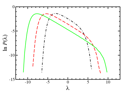
Figure 4: (color online) $\ln{P}(\lambda)$ for $\omega/\omega_{p}=0.5$, $C^{g}/C=0.01$, $\sigma_{S}^{2}=0.01$, $\sigma_{g}^{2}=0$, and the quality factor $Q=10^{5},10^{6},10^{7}$ (the dot-dashed, dashed, and solid curves, respectively), corresponding to $\kappa\xi=4.6\times{10}^{-2},4.6\times{10}^{-3},4.6\times{10}^{-4}$, respectively.

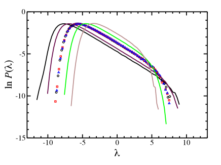
Figure 5: (color online) $\ln{P}(\lambda)$ for $\omega/\omega_{p}=0.8$, $C^{g}/C=0.01$ and $Q=2\times{10}^{6}$. The three sets of symbols represent the distributions for $\sigma_{S}^{2}=0.01$, $\sigma_{g}^{2}=0$ (circles), $\sigma_{S}^{2}=0.005$, $\sigma_{g}^{2}=0.005$ (squares), and $\sigma_{S}^{2}=0$, $\sigma_{g}^{2}=0.01$ (triangles), all corresponding to $\kappa\xi=3.3\times{10}^{-3}$. They collapse to one curve, showing that the distribution is sensitive only to the combination $\sigma_{S}^{2}+\sigma_{g}^{2}$. The solid curves represent the distributions for $\sigma_{g}^{2}=0$ and $\sigma_{S}^{2}=0.05,\;0.03,\;0.003\;0.001$ (the curves with the longer flat part corresponding to larger $\sigma_{S}^{2}$), for which the parameter $\kappa\xi=6.6\times{10}^{-4},\;1.1\times{10}^{-3},\;1.1\times{10}^{-2},\;3.3\times{10}^{-2}$, respectively.

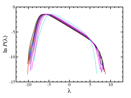
Figure 6: (color online) $\ln{P}(\lambda)$ for $C^{g}/C=0.05$, $Q=10^{5}$, $\sigma_{S}^{2}=0.05$, $\sigma_{g}^{2}=0$, and $\omega/\omega_{p}=0.1,\,0.2,\,0.3,\,0.4,\,0.5,\,0.6,\,0.7,\,0.8,\,0.9,\,0.99$. corresponding to $\kappa\xi=3.60\times{10}^{-3},\,3.65\times{10}^{-3},\,3.75\times{10}^{-3},\,3.90\times{10}^{-3},\,4.12\times{10}^{-3},\,4.46\times{10}^{-3},\,4.98\times{10}^{-3},\,5.90\times{10}^{-3},\,7.99\times{10}^{-3},\,1.57\times{10}^{-2}$, respectively. The curves with the longer flat part correspond to lower frequencies.

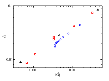
Figure 7: (color online) The coefficient $A$ in Eq. (65) versus the parameter $\kappa\xi$ for the distributions shown in Fig. 4 (triangles), Fig. 5 (squares) and Fig. 6 (circles).

VII Conclusions

In this paper, we analyzed the properties of the normal modes of a chain of Josephson junctions in the superconducting regime, in the simultaneous presence of disorder and absorption. We considered the limit where disorder and absorption can be treated additively and computed the frequency shift and the localization length of the modes. We also calculated the distribution of the frequency-dependent impedance of the chain. The statistics depend on the parameter $\kappa\xi$, the ratio of the localization length and the absorption length. If $\kappa\xi\gg 1$, the modes within one localization length are much broadened by absorption and strongly overlap. This is the regime of weak fluctuations; the distribution is Gaussian. In the opposite limit of little broadening, the modes present within one localization length are well separated in frequency and fluctuations are strong; the distribution has a power law tail.

The frequency-dependent impedance of Josephson junction chains can be probed experimentally in principle, e.g., by incorporating the chain in a resonator which is capacitively coupled to a co-planar wave guide (CPW) Masluk2012 . Microwave transmission experiments on the CPW enable one to probe the small oscillation modes of the chain directly. Alternatively, one could include a weaker junction with a small Josephson energy (a so-called black-sheep junction Manucharyan2012 ) into the chain, and measure its dc current-voltage characteristics. The low-voltage dc response yields information about the ac impedance of the chain at frequencies $\sim 2eV/\hbar$, as discussed in detail in Appendix D.

Finally, Josephson junction chains have been predicted to constitute quantum phase-slip (QPS) elements Matveev2002 . Recent experiments have provided evidence for the occurrence of QPS in Josephson junction chains Pop2010 ; Manucharyan2012 ; Haviland2013 . Phase-slip elements are of interest for applications Mooij2006 , e.g., as qubits for quantum information processing Astafiev2012 and as a current standard for quantum metrology Guichard2010 . A typical quantum phase-slip event generally excites the normal modes of the chain, therefore the QPS amplitude strongly depends on spectral properties of the modes Rastelli2012 . It would be interesting to calculate the QPS amplitude for disordered Josephson chains. In the presence of disorder the phase-slip process could be decoupled from part of the modes, a fact that might well result in an enhancement of the phase-slip amplitude.

VIII Acknowledgements

We thank G. Crisan, A. DiMarco, V. Golovach, W. Guichard, G. Rastelli, and T. Ziman for useful discussions. We acknowledge financial support from the European network SOLID, from Institut universitaire de France, and from the European Research Council (grant “FrequJoc” No. 306731).

Appendix A Relation between impedance and reflection

To define the amplitude reflection coefficient of a Josephson junction chain, one should consider the system (2) with all $I_{n}=0$, replace the part of the chain to the left of the island $n=N_{1}$ by an effective impedance $Z_{\infty}$, and assume the part of the chain on the right to be disorder-free and dissipationless. Thus, the equation for $n=N_{1}$ should be replaced by the effective boundary condition

$$\left(-\frac{1}{i\omega{L}}-i\omega{C}\right)(V_{N_{1}}-V_{N_{1}+1})+\frac{V_{N_{1}}}{Z_{\infty}}=0,\quad$$ (66)

and the solution of the system for $n\geq{N}_{1}$ should be sought in the form $V_{n}=e^{-ik(n-N_{1})}+re^{ik(n-N_{1})}$, where the wave vector $k$ is related to the frequency $\omega$ by the dispersion relation (6) at $Q\to\infty$. This gives

$$r=-\frac{1+i\omega{C}^{g}Z_{\infty}\displaystyle[\epsilon_{\omega}+i\sqrt{1-(1-\epsilon_{\omega})^{2}}]/(2\epsilon_{\omega})}{1+i\omega{C}^{g}Z_{\infty}[\epsilon_{\omega}-i\sqrt{1-(1-\epsilon_{\omega})^{2}}]/(2\epsilon_{\omega})},$$ (67)

where $\epsilon_{\omega}\equiv(\omega^{2}LC^{g}/2)/(1-\omega^{2}LC)$. If $Z_{\infty}$ is real, then $|r|=1$. Otherwise,

$$1-|r|^{2}=\frac{2\sqrt{1-(1-\epsilon_{\omega})^{2}}\,\omega{C}^{g}\mathop{\mathrm{Re}}\nolimits{Z}_{\infty}}{\sqrt{1-(1-\epsilon_{\omega})^{2}}\,\omega{C}^{g}\mathop{\mathrm{Re}}\nolimits{Z}_{\infty}+\epsilon_{\omega}-\epsilon_{\omega}\omega{C}^{g}\mathop{\mathrm{Im}}\nolimits{Z}_{\infty}+|\omega{C}^{g}Z_{\infty}|^{2}/2}.$$ (68)

The one-to-one correspondence between $Z_{\infty}$ and $r$, expressed by Eq. (67), implies that the numerical results of Sec. VI for the distribution of $\mathop{\mathrm{Re}}\nolimits{Z}_{\infty}$ in the regime $\kappa\xi\ll{1}$ can be straightforwardly translated into the distribution of $|r|^{2}$, which turns out to have a power-law tail $\propto(1-|r|^{2})^{-2.0}$, in agreement with Ref. PradhanKumar, .

Appendix B Probability distribution of a sum of Lorentzians

Instead of the probability distribution function, we first calculate its Laplace transform called the characteristic function,

$$\begin{split}\mathcal{Q}(s)\equiv{}&{}\int\limits_{0}^{\infty}{e}^{-sx}P(x)\,dx=\\ ={}&{}\int\limits_{-\Delta/2}^{\Delta/2}\frac{d\omega_{1}}{\Delta}\ldots\frac{d\omega_{N_{\xi}}}{\Delta}\,\exp\left(-\sum_{\alpha=1}^{N_{\xi}}\frac{s\delta_{\xi}\gamma/\pi}{\omega_{\alpha}^{2}+\gamma^{2}}\right),\end{split}$$ (69)

where we have shifted the integration variables by $\omega$. The $N_{\xi}$-fold integral is factorised into a product of $N_{\xi}$ identical integrals. Recalling that $N_{\xi}=\Delta/\delta_{\xi}$ we represent each such integral as

$$\begin{split}&\int\limits_{-N_{\xi}\delta_{\xi}/2}^{N_{\xi}\delta_{\xi}/2}\frac{d\omega_{1}}{N_{\xi}\delta_{\xi}}\,\exp\left(-\frac{s\delta_{\xi}\gamma/\pi}{\omega_{1}^{2}+\gamma^{2}}\right)=\\ &=1-\frac{\gamma}{N_{\xi}\delta_{\xi}}\int\limits_{-\infty}^{\infty}{d}y\left\{1-\exp\left[-\frac{s\delta_{\xi}/(\pi\gamma)}{y^{2}+1}\right]\right\},\end{split}$$ (70)

where we introduced the dimensionless variable $y=\omega_{1}/\gamma$ and used the fact that the exponential is different from unity only limits of the last integral to infinity. Since this last integral no longer depends on $N_{\xi}$, the characteristic function can be represented as

$$\mathcal{Q}(s)=\left(1-\frac{\mathcal{F}(s)}{N_{\xi}}\right)^{N_{\xi}}\approx{e}^{-\mathcal{F}(s)},$$ (71)

where we took the limit $N_{\xi}\to\infty$. The function $\mathcal{F}(s)$ can be calculated exactly:

$$\begin{split}\mathcal{F}(s)&=\frac{\gamma}{\delta_{\xi}}\int\limits_{-\infty}^{\infty}{d}y\int\limits_{0}^{s\delta_{\xi}/(\pi\gamma)}\frac{e^{-z/(y^{2}+1)}dz}{y^{2}+1}=\\ {}&{}=\frac{\pi\gamma}{\delta_{\xi}}\int\limits_{0}^{s\delta_{\xi}/(\pi\gamma)}e^{-z/2}I_{0}(z/2)\,dz=\\ {}&{}=s\exp\left(-\frac{s\delta_{\xi}}{2\pi\gamma}\right)\left[I_{0}\!\left(\frac{s\delta_{\xi}}{2\pi\gamma}\right)+I_{1}\!\left(\frac{s\delta_{\xi}}{2\pi\gamma}\right)\right],\end{split}$$ (72)

where $I_{0},I_{1}$ are the modified Bessel functions. This immediately gives us access to the moments of $P(x)$:

$$\langle{1}\rangle=e^{-\mathcal{F}(0)}=1,$$ (73a)

$$\langle{x}\rangle=\mathcal{F}^{\prime}(0)=1,$$ (73b)

$$\langle{x}^{2}\rangle-\langle{x}\rangle^{2}=-\mathcal{F}^{\prime\prime}(0)=\frac{\delta_{\xi}}{2\pi\gamma}.$$ (73c)

The first two equations are trivial (recall that we have defined $x$ relative to the average value), but the last one already tells us that the fluctuations become large when $\delta_{\xi}/\gamma\gg{1}$.

To obtain the distribution function $P(x)$, we have to perform the inverse Laplace transform of $e^{-\mathcal{F}(s)}$. Unable to do it for the exact expression (72), we use two asymptotic expressions:

$$\mathcal{F}(s)=\left\{\begin{array}[]{ll}s-s^{2}\delta_{\xi}/(4\pi\gamma),&s\delta_{\xi}/\gamma\ll{1},\\ \sqrt{4s\gamma/\delta_{\xi}},&s\delta_{\xi}/\gamma\gg{1}.\end{array}\right.$$ (74)

The most important values of $s$ for the reconstruction of $P(x)$ are those for which $\mathcal{F}(s)\sim{1}$, that is, $s\sim\max\{1,\delta_{\xi}/\gamma\}$. Thus, the first expression from Eq. (74) is good for the limit $\delta_{\xi}\ll\gamma$, while the second one is good when $\delta_{\xi}\gg\gamma$. One can check the that the inverse Laplace transforms of $e^{-\mathcal{F}(s)}$ for the two expressions are given by

$$P(x)=\sqrt{\gamma/\delta_{\xi}}\,e^{-(\pi\gamma/\delta_{\xi})(x-1)^{2}},\delta_{\xi}\ll\gamma,$$ (75a)

$$P(x)=\frac{e^{-\gamma/(x\delta_{\xi})}}{\sqrt{\pi(\delta_{\xi}/\gamma)x^{3}}},\quad\delta_{\xi}\gg\gamma.$$ (75b)

For the first expression the check is straightforward, while for the second one we have (rescaling $s\to{s}\gamma/\delta_{\xi}$)

$$\begin{split}&\int\limits_{0}^{\infty}\frac{e^{-1/y-sy}}{\sqrt{\pi{y}^{3}}}\,dy=\quad(y=e^{2t})\\ &=\frac{2}{\sqrt{\pi}}\int\limits_{-\infty}^{\infty}\exp\left(-t-e^{-2t}-se^{2t}\right)dt=\quad\left(t\to{t}-\frac{\ln{s}}{4}\right)\\ &=\frac{2s^{1/4}}{\sqrt{\pi}}\int\limits_{-\infty}^{\infty}e^{-t-2\sqrt{s}\cosh{2}t}dt=\\ &=\frac{4s^{1/4}}{\sqrt{\pi}}\int\limits_{0}^{\infty}e^{-2\sqrt{s}\cosh{2t}}\cosh{t}\,dt=\quad(\sinh{t}=u)\\ &=\frac{4s^{1/4}}{\sqrt{\pi}}\int\limits_{0}^{\infty}e^{-2\sqrt{s}(2u^{2}+1)}\,du=e^{-\sqrt{4s}}.\end{split}$$ (76)

While Eq. (75a) is good enough and coincides with Eq. (20a), the distribution in Eq. (75b) has all moments divergent, as a consequence of the non-analyticity of $\mathcal{F}(s)=\sqrt{4s\gamma/\delta_{\xi}}$ at $s\to{0}$. This non-analyticity is an artefact of the asymptotic expression we have used, which loses its validity at small $s\sim\gamma/\delta_{\xi}$, while the exact $\mathcal{F}(x)$ from Eq. (72) is always analytic at $s\to{0}$. In terms of $P(x)$, this means that the large-$x$ tail $P(x)\propto{x}^{-3/2}$ should be cut off at $x\sim\delta_{\xi}/\gamma$.

The cutoff can be easily obtained directly from the definition of $P(x)$, Eq. (19), by noting that large $x$ corresponds to $\omega$ being close to one of the Lorentzians. Neglecting the probability of overlap of two Lorentzians, and noting that any of the $N_{\xi}$ Lorentizans can be close to $\omega$, we obtain

$$\begin{split}P(x){}&{}=N_{\xi}\int\limits_{-\infty}^{\infty}\frac{d\omega}{\Delta}\,\delta\!\left(x-\frac{\delta_{\xi}\gamma/\pi}{\omega^{2}+\gamma^{2}}\right)=\\ {}&{}=\frac{1}{\pi{x}^{3/2}\sqrt{\delta_{\xi}/(\pi\gamma)-x}},\end{split}$$ (77)

valid for $x\gg\gamma/\delta_{\xi}$ (which is the typical value of $x$ between the Lorentzians). The previous expression, Eq. (75b), is valid for $0<x\ll\delta_{\xi}/\gamma$. Thus, the two expressions are both valid in the wide region $\gamma/\delta_{\xi}\ll{x}\ll\delta_{\xi}/\gamma$, where they both reduce to $1/\sqrt{\pi(\delta_{\xi}/\gamma)x^{3}}$. Combining the two, we arrive at Eq. (20b).

Appendix C Damped harmonic oscillator

Consider the Hamiltonian equations for a damped harmonic oscillator of the mass $m$ and eigenfrequency $\omega_{0}$, subject to an external force $f(t)$:

$$\frac{dp}{dt}=-m\omega_{0}^{2}x-2\gamma{p}+f(t),$$ (78a)

$$\frac{dx}{dt}=\frac{p}{m},$$ (78b)

$2\gamma$ being the damping rate. Assuming the force to be monochromatic and looking for the solutions $\propto{e}^{-i\omega{t}}$, we obtain the equation

$$(\omega_{0}^{2}-2i\gamma\omega-\omega^{2})\,p=-i\omega{f},$$ (79)

which is the analog of Eq. (23). The analog of Eq. (25) is then

$$\left(\omega-\hat{\mathcal{A}}\right)\left(\begin{array}[]{c}p\\ w\end{array}\right)=\left(\begin{array}[]{c}if\\ 0\end{array}\right)$$ (80)

with the matrix $\hat{\mathcal{A}}$ given by

$$\hat{\mathcal{A}}=\left(\begin{array}[]{cc}-2i\gamma&\omega_{0}\\ \omega_{0}&0\end{array}\right).$$ (81)

The auxiliary variable $w$ is nothing but $w=-ix$.

The matix $\hat{\mathcal{A}}$ has two non-degenerate eigenvalues

$$-i\gamma\pm\sqrt{\omega_{0}^{2}-\gamma^{2}},$$

except for the special case $\gamma=\omega_{0}$. In this case there is one doubly degenerate eigenvalue, and the matix $\hat{\mathcal{A}}$ has only one eigenvector. For $\gamma<\omega_{0}$ (weak damping), the two eigenvalues can be denoted by $\omega_{1}$ and $-\omega_{1}^{*}$. The normalization condition, analogous to Eq. (32),

$$p_{1}^{2}\left(1+\frac{\omega_{0}^{2}}{\omega_{1}^{2}}\right)=1,$$ (82)

determines the oscillator moblity $b=f/p$, which is analogous to the impedance in Eq. (33):

$$b(\omega)=\frac{ip_{1}^{2}}{\omega-\omega_{1}}+\frac{i(p_{1}^{*})^{2}}{\omega+\omega_{1}^{*}}=\frac{i\omega}{\omega^{2}-2i\gamma\omega-\omega_{0}^{2}},$$ (83)

which, of course, also follows directly from Eq. (79).

Appendix D Current-voltage characteristic of a black-sheep junction coupled to a Josephson chain

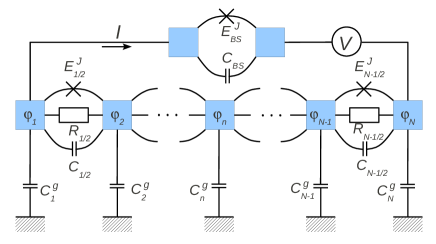
Figure 8: (color online) A schematic view of the black-sheep scheme of impedance measurement.

We consider a voltage-biased circuit (bias voltage $V$) containing a black-sheep (BS) junction with capacitance $C_{BS}$ and Josephson coupling energy $E_{J,BS}$ in series with a Josephson junction chain (Fig. 8). In the absence of quasiparticles, a small dc voltage bias $V$ is expected to induce a Cooper pair current $I(V)$. The necessary dissipation is provided by the broadened modes of the Josephson junction chain. For small $E_{J,BS}$, a perturbative calculation yields Ingold1992

$$I(V)=\frac{\pi eE_{J,BS}^{2}}{\hbar}[P(2eV)-P(-2eV)].$$ (84)

Here we defined the function $P(E)$ as

$$P(E)=\frac{1}{2\pi\hbar}\int dt\,e^{J(t)+iEt/\hbar},$$ (85)

with

$$\begin{split}J(t)={}&{}8\int\limits_{0}^{\infty}\frac{d\omega}{\omega}\,\frac{\mathop{\mathrm{Re}}\nolimits[Z_{\mathrm{tot}}(\omega)]}{R_{K}}\times\\ {}&{}\times\left\{[\cos(\omega t)-1]\coth\frac{\beta\hbar\omega}{2}-i\sin(\omega t)\right\},\end{split}$$ (86)

where $R_{K}=h/e^{2}$. The chain is kept at the inverse temperature $\beta=1/k_{B}T$; the impedance $Z_{\mathrm{tot}}$ is the total impedance ”seen” by the BS junction: a parallel arrangement of the junction capacitance $C_{BS}$ and the impedance $Z(\omega)$ of the chain. Hence,

$$\mathop{\mathrm{Re}}\nolimits[Z_{\textrm{tot}}(\omega)]=\frac{\mathop{\mathrm{Re}}\nolimits[Z(\omega)]}{|1-i\omega C_{BS}Z(\omega)|^{2}}\ .$$ (87)

An interesting case is the so-called weak-coupling limit, where $J(t)$ remains small on the relevant time scales, such that

$$P(E)\simeq\frac{1}{2\pi\hbar}\int_{-\infty}^{+\infty}dt\,e^{iEt/\hbar}\,[1+J(t)].$$ (88)

This corresponds to the case where the BS junction exchanges at most one photon with the chain. Indeed, the evaluation of the integral over time in (88) gives

$$\begin{split}&P(E)\simeq\delta(E)+8\int_{0}^{+\infty}\frac{d\omega}{\omega}\,\frac{\mathop{\mathrm{Re}}\nolimits[Z_{\textrm{tot}}(\omega)]}{R_{K}}\times\\ &\times\left[n_{\omega}\delta(E+\hbar\omega)+(n_{\omega}+1)\delta(E-{\hbar}\omega)-(2n_{\omega}+1)\delta(E)\right],\end{split}$$ (89)

where $n_{\omega}=1/(e^{\beta\hbar\omega}-1)$ is the Bose-Einstein distribution function. The first and the fourth terms represent elastic Cooper pair tunnelling in the BS junction involving zero and one virtual photon, respectively. The second and third terms are related to the process of absorption and emission of one real photon, respectively.

As can be seen from Eq. (84), the calculation of the current-voltage characteristic involves the inelastic part of $P(E)$ only, given by

$$P(E)\simeq\ 8\ \frac{\mathop{\mathrm{Re}}\nolimits[Z_{\textrm{tot}}(E/\hbar)]}{R_{K}}\,\frac{1+n_{E/\hbar}}{E}.$$ (90)

Substituting Eq. (90) into Eq. (84) then yields the current-voltage characteristic in the weak-coupling limit,

$$I(V)\simeq\frac{4\pi E_{J,BS}^{2}}{\hbar V}\frac{\mathop{\mathrm{Re}}\nolimits[Z_{\textrm{tot}}(2eV/\hbar)]}{R_{K}}\ .$$ (91)

Note that the DC current at voltage $V$ directly probes the environmental impedance $Z_{\textrm{tot}}$ at frequency $\omega=2eV/\hbar$. Specifically, at low frequencies, the chain tends to become purely inductive, $\mathop{\mathrm{Re}}\nolimits[Z(\omega\to 0)]\simeq N\omega^{2}\langle L^{2}\rangle/R$ with $N$ the number of junctions, $\langle L^{2}\rangle$ the average squared Josephson inductance of the chain and $R$ the junction resistance. Hence $\mathop{\mathrm{Re}}\nolimits[Z_{\textrm{tot}}(\omega\to 0)]\simeq N\omega^{2}\langle L^{2}\rangle/R$. As a result, at low voltage the current-voltage characteristic vanishes linearly with $V$. At high frequencies, capacitive behavior takes over and for frequencies above the plasma frequency the impedance tends tend to zero again. Hence the current also vanishes at high voltages. Between zero and the plasma frequency, $\mathop{\mathrm{Re}}\nolimits[Z_{\textrm{tot}}(\omega)]$ presents a series of $N$ peaks, corresponding to the chain’s modes. These will appear as current peaks in the current-voltage characteristics.

References

- (1) M. Watanabe and D. B. Haviland, Phys. Rev. Lett. 86, 5120 (2001).
- (2) S. Corlevi, W. Guichard, F. W. J. Hekking, and D. B. Haviland, Phys. Rev. Lett. 97, 096802 (2006).
- (3) S. Corlevi, W. Guichard, F. W. J. Hekking, and D. B. Haviland, Phys. Rev. B 74, 224505 (2006).
- (4) V. E. Manucharyan, J. Koch, L. I. Glazman, and M. H. Devoret, Science 326, 113 (2009).
- (5) N. A. Masluk, I. M. Pop, A. Kamal, Z. K. Minev, and M. H. Devoret, Phys. Rev. Lett. 109, 137002 (2012).
- (6) M. T. Bell, I. A. Sadovskyy, L. B. Ioffe, A. Y. Kitaev, and M. E. Gershenson, Phys. Rev. Lett. 109, 137003 (2012).
- (7) R.M. Bradley and S. Doniach, Phys. Rev. B 30, 1138 (1984).
- (8) E. Chow, P. Delsing, and D.B. Haviland, Phys. Rev. Lett. 81, 204 (1998).
- (9) D.B. Haviland, K. Andersson, and P. Agren, J. Low Temp. Phys. 118, 733 (2000).
- (10) W. Kuo and C.D. Chen, Phys. Rev. Lett. 87, 186804 (2001).
- (11) H. Miyazaki, Y. Takahide, A. Kanda, and Y. Ootuka, Phys. Rev. Lett. 89, 197001 (2002).
- (12) Y. Takahide, H. Miyazaki, and Y. Ootuka, Phys. Rev. B 73, 224503 (2006).
- (13) R. Fazio and H. S. J. van der Zant, Phys. Rep. 355, 235 (2001).
- (14) F.J. Dyson, Physical Review 92, 1331 (1953).
- (15) T. Ziman, Phys. Rev. Lett. 49, 337 (1982).
- (16) K. K. Likharev, Dynamics of Josephson junctions and circuits, Gordon and Breach publishers, Amsterdam, The Netherlands (1986).
- (17) G. Schön and A.D. Zaikin, Phys. Rep. 198, 237 (1990).
- (18) V. Freilikher, M. Pustilnik, and I. Yurkevich, Phys. Rev. Lett. 73, 810 (1994).
- (19) P. Pradhan and N. Kumar, Phys. Rev. B 50, 9644 (1994).
- (20) N. A. Bruce and J. T. Chalker, J. Phys. A: Math. Gen. 29, 3761 (1996).
- (21) C. W. J. Beenakker, J. C. J. Paasschens, and P. W. Brouwer, Phys. Rev. Lett. 76, 1368 (1996).
- (22) T. Sh. Misirpashaev and C. W. J. Beenakker, JETP Lett. 64, 319 (1996).
- (23) L. I. Deych, A. Yamilov, and A. A. Lisyansky, Phys. Rev. B 64, 024201 (2001).
- (24) G. Rastelli, I. M. Pop, and F.W.J. Hekking, Phys. Rev. B 87, 174513 (2013).
- (25) S. John, H. Sompolinsky, and M.J. Stephen, Phys. Rev. B 27, 5592 (1983).
- (26) V. Gurarie and J. T. Chalker, Phys. Rev. B 68, 134207 (2003).
- (27) N. Bilas and N. Pavloff, Eur. Phys. J. D 40, 387 (2006).
- (28) G. Crisan, Theoretical study of the impedance of disordered Josephson junction chains, Master thesis at Babes-Bolyai University (Cluj-Napoca, 2013).
- (29) I. M. Lifshitz, S. A. Gredeskul, and L. A. Pastur, Introduction to the Theory of Disordered Systems (Wiley, New York, 1988).
- (30) P. A. Mello and N. Kumar, Quantum Transport in Mesoscopic Systems: Complexity and Statistical Fluctuations (Oxford University Press, London, 2004).
- (31) Strictly speaking, this is correct only for values of , which are incommensurate with . For commensurate values, the averaging is poor, which leads to the so-called anomalies [B. Derrida and E. Gardner, J. Phys. (Paris) 45, 1283 (1984); V. E. Kravtsov and V. I. Yudson, Ann. Phys. 326, 1672 (2011)], the strongest and the most studied one one being at [L. P. Gorkov and O. N. Dorokhov, Solid State Commun. 20, 789 (1976); G. Czycholl, B. Kramer, and A. MacKinnon, Z. Phys. B 43, 5 (1981); M. Kappus and F. Wegner, Z. Phys. B 45, 15 (1981); H. Schomerus and M. Titov, Phys. Rev. B 67, 100201(R) (2003); V. E. Kravtsov and V. I. Yudson, Phys. Rev. B 82, 195120 (2010); V. E. Kravtsov and V. I. Yudson, J. Phys. A 46, 025001 (2013)]. It is known to change the localization length by about 9% in the case of the one-dimensional Anderson model. Such anomalies are beyond the scope of the present paper.
- (32) N. G. Van Kampen, Stochastic Processes in Physics and Chemistry (Elsevier, Amsterdam, 2007).
- (33) V. E. Manucharyan, N. A. Masluk, A. Kamal, J. Koch, L. I. Glazman, and M. H. Devoret, Phys. Rev. B 85, 024521 (2012).
- (34) K. A. Matveev, A. I. Larkin, and L. I. Glazman, Phys. Rev. Lett. 89, 096802 (2002).
- (35) I.M. Pop, I. Protopopov, F. Lecocq, Z. Peng, B. Pannetier, O. Buisson, and W. Guichard, Nat. Phys. 6, 589 (2010).
- (36) A. Ergül, J. Lidmar, J. Johansson, Y. Azigoglu, D. Schaeffer, and D.B. Haviland, arXiv:1305.7157.
- (37) J.E. Mooij and Yu. V. Nazarov, Nat. Phys. 2, 169 (2006).
- (38) O. V. Astafiev, L. B. Ioffe, S. Kafanov, Y. A. Pashkin, K. Yu. Arutyunov, D. Shahar, O. Cohen, and J. S. Tsai, Nature 484, 355 (2012).
- (39) W. Guichard and F.W.J. Hekking, Phys. Rev. B 81, 064508 (2010).
- (40) G.-L Ingold and Yu. V. Nazarov, in Single Charge Tunneling, ed. by H. Grabert and M. H. Devoret, NATO ASI Series B, Vol. 294, pp. 21–107 (Plenum Press, New York, 1992).