Selective advantage of diffusing faster

Abstract

We study a stochastic spatial model of biological competition in which two species have the same birth and death rates, but different diffusion constants. In the absence of this difference, the model can be considered as an off-lattice version of the Voter model and presents similar coarsening properties. We show that even a relative difference in diffusivity on the order of a few percent may lead to a strong bias in the coarsening process favoring the more agile species. We theoretically quantify this selective advantage and present analytical formulas for the average growth of the fastest species and its fixation probability.

Different physical, social and biological systems can be described by models belonging to the Voter Model (VM) universality class dornic . An important example in biology is the neutral Stepping Stone Model 6 ; 7 whose dynamics explains qualitative and quantitatively spreading and fixation of competing populations on a Petri dish hall_exp ; korolev_sweeps . In statistical physics, the VM is characterized by the existence of two symmetric absorbing states and a coarsening process without surface tension. Its macroscopic dynamics corresponds to the Langevin equation

$$\partial_{t}f(\mathbf{x},t)=D\Delta f+\sqrt{\Gamma f(1-f)}\eta(\mathbf{x},t)$$ (1)

where $D$ is the diffusion constant, $\Gamma$ the noise amplitude and $\eta(\mathbf{x},t)$ is a $\delta$ -correlated white noise. In biological applications, the field $f$ usually represents the frequency of an allele, i.e., the local fraction of individuals carrying a given mutation. When mutants have a ”selective advantage” $s$ over the wild type (i.e. a difference in reproduction rate), an additional term appears in Eq. (1), which becomes a stochastic version of the celebrated Fisher-Kolmogorov-Petrovskii-Piscounov (FKPP) equation

$$\partial_{t}f(\mathbf{x},t)=D\Delta f+sf(1-f)+\sqrt{\Gamma f(1-f)}\eta(\mathbf{x},t)$$ (2)

In the absence of noise, Eq. (2) predicts a well-defined range expansion velocity of the mutants, $v=2\sqrt{Ds}$ fisher ; kolmogorov . The same result is valid in the presence of weak multiplicative noise, up to logarithmic corrections derrida ; pechenik , while in the strong noise regime one should expect a difference expression for the velocity doering ; hallat_strongnoise .

The stochastic FKPP equation is radically different from the VM. One can think of $s$ in a similar way as the external field in the Ising model, breaking the $f\leftrightarrow(1-f)$ symmetry and thus driving the system away from the critical point, which is recovered for $s=0$. For $s>0$, Eq.(2) predicts $f=1$ to be the deterministic asymptotic stable equilibrium of the system, the state $f=0$ being unstable. Often, the critical behaviors of Langevin equation such as variants of Eq. (1) can be understood by analyzing their corresponding deterministic dynamics, either by means of its associated mean field potential hammal or by the Hamiltonian dynamics obtained by the path integral formulations elgart .

Due to the relevance of the VM in non-equilibrium phenomena, it is interesting to understand whether there exists more general, possibly non-deterministic mechanisms to break the VM universality class. In biological terms, this amounts to ask whether an effective selective advantage can be achieved without any asymmetry in the birth and death rates. For example, it has been recently shown hall_noise that an asymmetry in the carrying capacity (i.e. the global biological mass) of the two alleles can induce an effective selective advantage.

In this Letter, we show that an effective selective advantage emerges in a competition model between two species diffusing at different speeds, but otherwise neutral. In biology, this setting is relevant to assess the evolutionary importance of movement, for example in species which exist in motile and non-motile variants, such as bacteria with and without flagellum. We will show that, in this case, competition is biased towards the fastest species. This is equivalent to an effective selective advantage which depends both on noise and spatial fluctuations, and is proportional to both the noise amplitude and the difference in diffusivity.

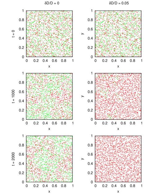
Figure 1: Snapshots of $2d$ configurations of the particle model at different times. In all panels, parameters are $N=10^{4}$ and $D=10^{-4}$. Details of the particle simulations are in suppl . (left column) The two species have the same diffusivity. (right column) The red species has diffusivity $D+\delta D$ with $\delta D/D=0.05$. To help the viewer, configurations has been downsampled (one every four particles, chosen at random, is shown).

We consider a model in which particles belonging to two different species $A$ and $B$ diffuse in space, reproduce according to the reactions $A\rightarrow 2A$ and $B\rightarrow 2B$, and die in a density-dependent fashion ($A+A/B\rightarrow A$ and $B+A/B\rightarrow A$) as result of competition. For simplicity, we assume all reactions to occur at the same rate $\mu=1$. The system is an hypercube of size $L^{d}$ in $d$ dimensions with periodic boundary conditions (see longpaper ; suppl for details on the implementation). We call $D+\delta D$ and $D$ the diffusion constants of species $A$ and $B$ respectively. When $\delta D=0$, the dynamics of the model is characterized by a coarsening process, as shown in the two-dimensional example of Fig. (1), left column. We will later argue that this coarsening belongs to the universality class of the VM. Instead, Fig. (1), right column shows that a small difference in the diffusivity of the two species, $\delta D/D=5\%$ in this case, imposes a non-negligible bias on the coarsening dynamics and, in particular, confers to an advantage to the species having a larger diffusivity. A similar behavior can be observed also in 1d simulations.

We derived macroscopic equations for the concentrations of the two species $c_{A}(\mathbf{x},t)$ and $c_{B}(\mathbf{x},t)$ gardiner ; prl_pigolotti ; longpaper ; suppl . The result is

$$\partial_{t}c_{A} = (D+\delta D)\nabla^{2}c_{A}+\mu c_{A}(1-c_{A}-c_{B})+\sigma_{A}\xi_{A}$$

$$\partial_{t}c_{B} = D\nabla^{2}c_{B}+\mu c_{B}(1-c_{A}-c_{B})+\sigma_{B}\xi_{B}$$ (3)

where $\sigma_{A}=\sqrt{\mu c_{A}(1+c_{A}+c_{B})/N}$ and similarly for $\sigma_{B}$. The parameter $\mu/N$ is the genetic drift and $N$ can be interpreted as the density of particles corresponding to a macroscopic concentration $c=1$. $\xi_{A}(\mathbf{x},t)$ and $\xi_{B}(\mathbf{x},t)$ are independent delta-correlated (in space and time) noise sources, $\langle\xi_{i}(\mathbf{x},t)\xi_{j}(\mathbf{x^{\prime}},t^{\prime})\rangle=\delta_{ij}\delta(\mathbf{x}-\mathbf{x^{\prime}})\delta(t-t^{\prime})$. An equation for the relative concentration of one species $f\equiv c_{A}/(c_{A}+c_{B})$ can be obtained from Eqs. (Selective advantage of diffusing faster) by means of Ito’s formula prl_pigolotti ; longpaper . Performing the calculation and neglecting fluctuations of the total particle density by imposing $c_{A}+c_{B}=1$ at the end of the procedure yields

$$\partial_{t}f(\mathbf{x},t)=D\nabla^{2}f+\delta D(1-f)\nabla^{2}f+\sigma\xi(\mathbf{x},t)$$ (4)

where $\sigma=\sqrt{2\mu f(1-f)/N}$. Eq. (4) constitutes the starting point of our analysis. We remark that, while we neglected fluctuations of the total density $c_{A}+c_{B}$, the fact that the total density is not strictly conserved is crucial to derive Eq. (4). This correspond to the fact that it is impossible to have two species with different diffusion constant in a lattice model: if each site is strictly occupied by one spin, then the effective diffusivity of the two species is equal by constraint. Setting $\delta D=0$ in (4) one retrieves Eq. (1) describing the VM universality class longpaper ; revmodph ; hammal . Although (4) has been derived thinking of the continuum limit of a biological model, we argue that its validity is more general, as the term proportional to $\delta D$ is the simplest, non-trivial way to account for a difference in diffusivity between the two species. In the following, we will study how this term affects the dynamics by breaking the the VM universality class.

We start by focusing on the $1d$ case and study the time evolution of the integrated mean concentration $F(t)=\langle f\rangle$, where $\langle..\rangle$ denotes an average over space and noise. From Eq. (4) we obtain

$$\frac{dF}{dt}=\delta D\ \langle(\nabla f)^{2}\rangle>0$$ (5)

which is Eq. (19). The above equation already shows that $F(t)$ is a growing function of time for any $\delta D>0$. The behavior of $F(t)$ is presented in Fig. (2) in $1d$ simulations of the particle model, starting with uniformly distributed populations but a more abundant slow species, so that $F(0)=0.1$. Notice how $F(t)$ decreases at increasing $N$ and increasing $D$ at constant $\delta D/D$. A straightforward calculation suppl shows that

$$\frac{dF(t)}{dt}=\frac{\delta D}{2}\nabla^{2}H(x,t)|_{x=0}$$ (6)

where we introduced the two point connected correlation function (heterozygosity in biological language) $H(x=x_{1}-x_{2},t)=\langle f(x_{1})[1-f(x_{2})]+f(x_{2})[1-f(x_{1})]\rangle$, which is function of $x_{1}-x_{2}$ only due to translational invariance. For $\delta D=0$ the function $H(x,t)$ is explicitly known revmodph . For $\delta D/D\ll 1$, we can use this result to evaluate the right hand side of Eq. (6) perturbatively , i.e. by replacing the average $\langle\dots\rangle$ with the average $\langle\dots\rangle_{0}$ over the solvable case of $\delta D=0$ suppl . The result is

$$\frac{dF(t)}{dt}=\frac{\delta D}{4D\sqrt{\pi\epsilon t_{f}}}H(0){G(t/t_{f})}$$ (7)

where $G(x)=\exp(x)\mathrm{erfc}(\sqrt{x})$, $t_{f}=2DN^{2}$ and the parameter $\epsilon$ is an ultraviolet cutoff that can be assumed to be of order 1.

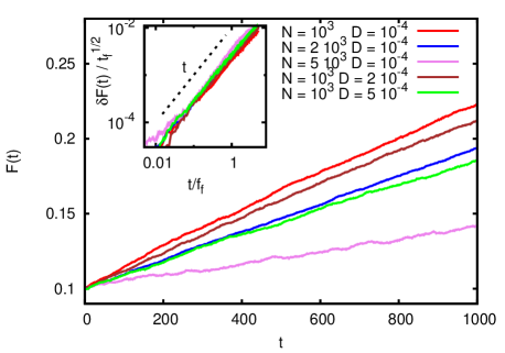
Figure 2: Behavior of the average concentration of the fast species $F(t)$ ar varying the number density $N$ and the diffusion constant of the slowest species $D$ in one dimension. In all simulations, the relative difference of diffusion constants is $\delta D/D=0.1$, the initial fraction of the fast species is $F(0)=0.1$ and the system size is $L=10$. Curves are average over $10^{3}$ realizations. The inset shows a data collapse according to Eq. (8). Linear scaling (black dashed line) is shown for comparison.

Using expression (7), we can cast the growth of $\delta F(t)=F(t)-F(0)$ into the scaling form

$$\delta F(t)=H(0)\sqrt{t_{f}}\frac{\delta D}{D}\phi(t/t_{f})$$ (8)

where the scaling function $\phi$ does not depend on parameters and is $\phi(x)\sim x$ for small $x$. A collapse of curves for different values of $N$ and $D$ according to (8), presented in the inset of Fig. (2), supports our theory within statistical fluctuations. Notice that, at this order in perturbation theory, the presence of absorbing states is not predicted by Eq. (7). This means that the perturbative approach is expected to describe properly the dynamics only on times shorter than the global fixation time, i..e. $L^{2}/D$.

It is of interest to compare a difference in diffusivity to a selective advantage caused by a difference $s$ in reproduction rates, i.e. in the case of equation (2). Assuming $s\ll 1$ and averaging directly such term, one obtains that $F(t)$ evolves in this case according to $dF/dt=sH(0)G(t/t_{f})/2$. Comparing the latter expression with Eq. (7), it is natural to define an effective advantage given by

$$s_{eff}=\frac{\delta D}{2D\sqrt{\epsilon\pi t_{f}}}.$$ (9)

To tackle the problem in higher dimensions, let us start from the general evolution equation for the two point connected correlation function as obtained from Eq. (4) for $\delta D=0$:

$$\partial_{t}H(x,t)=2D\nabla^{2}H-\frac{2\mu}{N}H(0,t)\delta(x).$$ (10)

Due to the spatial regularization doering , the delta function resulting from Ito calculus must be interpreted as $\delta(x)\sim 1/a^{d}$, where $a\sim\sqrt{2D\epsilon}$ is the lattice spacing of the discrete stepping stone model. In an adiabatic approximation of Eq. (10), $\nabla^{2}H|_{x=0}$ can be estimated as

$$\nabla^{2}H|_{x=0}\sim\frac{\mu H(0,t)}{DN(D\epsilon)^{d/2}}$$ (11)

which is consistent with the scaling of Eq. (8) for $d=1$. Evaluating Eq. (11) in $d=2$ yields $\nabla^{2}H|_{x=0}\sim\mu H(0,t)/(ND^{2}\epsilon)$, i.e. the effective advantage becomes larger by a factor $1/\sqrt{D\epsilon}$ with respect to the one dimensional case.

The interpretation of Eqs. (9) and (11) is that, after averaging over noise and space, the effect of a different diffusivity is analogous to that of a selective advantage. We now discuss the consequences for the peculiar coarsening properties of the VM. In $2D$, the dynamics of the VM is characterized by a slow coarsening process where the density of interface decays as $\log^{-1}(t)$ (see e.g. dornic ). In the continuum off-lattice case, the analogous of the density of interface is the local heterozigosity $H(x=0,t)$. Fig. (3) shows how $H(x=0,t)$ displays the expected logarithmic decay in our particle model. When either a selective advantage or a diffusivity difference is present, this behavior is observed up to a time $\bar{t}$ (either proportional to the selective advantage $s$ or the diffusivity difference $\delta D$) after which $H(0,t)$ decays exponentially. This shows how both terms have a similar effect in driving the dynamics away from the VM critical point.

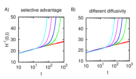
Figure 3: Comparison of the coarsening dynamics in $2D$ in the presence of A) selective advantage (i.e. faster reproduction rate of species A, and B) difference in diffusivity. Parameters are $D=2\cdot 10^{-5}$ and $N=4\cdot 10^{4}$; the system is a square of side $L=1$. In A), the selective advantage $s=0$ (red curve), $s=0.05,0.01,0.02,0.04$ (curves from right to left). In B) we vary $\delta D/D=0$ (red curve), $\delta D/D=0.04,0.08,0.16,0.32$ (curves from right to left). In both panels, we plot the inverse density of interfaces $H^{-1}(x=0,t)$ as a function of time. Notice how the logarithmic behaviour, characteristic of the VM is cut off on a time set by either the selective advantage or the difference in diffusivity.

The effective selective advantage introduced in Eq. (9) can be used to study the probability of fixation $P_{fix}$, defined as the probability of reaching the absorbing state $f=1$ of Eq. (4). The fixation probability in terms of a selective advantage is given by the formula doering ; longpaper

$$P_{fix}(s)=\frac{1-\exp(-2sNF(0))}{1-\exp(-2sN)}.$$ (12)

Assuming the same formula to hold in the case of different diffusivities with $s_{eff}$ replacing $s$ leads to an interesting prediction: $P_{fix}$ should not depend on $N$ as $s_{eff}\propto N^{-1}$. In Fig. (4A) we show $P_{fix}$ as a function of $\delta D/D$ for different values of $N$, confirming this prediction. The black line is the expression for $P_{fix}$, namely: obtained from $\epsilon\approx 0.5\mu^{-1}$. This also confirms our initial assumption of $\epsilon\mu\sim 1$. Notice how the bias in the fixation probabilities shown in Fig. (4) is much stronger in $2d$ than in $1d$ at equal parameter values, as predicted by Eq. (11)

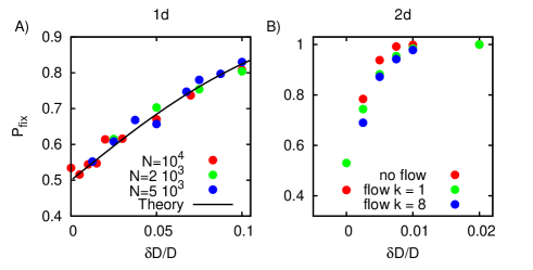
Figure 4: (A) Fixation probabilities in 1d. The black line is the theoretical prediction of Eq. (12). (B) Fixation probabilities in 2d, with and without fluid flow. In both panels we set $D=10^{-4}$.

We now briefly discuss the same problem in the presence of advection. Simulations in 2D shown in Fig. (4B) show similar fixation probabilities with and without advection by an incompressible flow (details in suppl ). In suppl we argue that in an incompressible flow Eq. (19) formally holds, leading to the same effective advantage for the species with larger diffusivity, as far as the typical scale of turbulent scale is not too small.

To conclude, we have shown that a small difference in diffusivity can induce a breaking of the VM universality class with the critical parameter proportional to the noise amplitude. In the framework of population dynamics, this means that a difference in diffusivity between two species can bias the outcome of competition towards the more agile one. Notice that, while in the presence of a range expansion there exist an advantage for the fastest species which can be estimated by looking at the difference between the deterministic Fisher velocities korolev_sweeps ; benichou , the effect presented here is genuinely stochastic and constitutes a new example of a noise-induced advantage in population genetics hall_noise ; heinsalu .

When considering a realistic biological scenario, the effective advantage given by a higher motility must be compared with its involved metabolic cost. In this respect, our result is reminiscent of a classic analysis of seed dispersal by Hamilton and May hamilton1 ; hamilton2 , which predicts an equilibrium, optimal level of dispersal even in an homogeneous environment. Further, our preliminary results in the presence of fluid flows suggest that the same effect can be crucial also in turbulent marine environments. We expect our result to be also relevant in other fields where diffusion is known to affect crucially the dynamics, such as chemical kinetics krap , game theory frey , and synchronization diaz . Indeed, a term proportional to $(1-f)\nabla^{2}f$ would generally appear in the continuous description of systems characterized by two spatial concentrations diffusing at different speed, the proper dynamical evolution being described by Eq. (4).

I Supplementary Material

II Particle model and macroscopic equations

II.1 Particle model

The particle model is implemented as follow. We consider particle belonging to two different species, $A$ and $B$. All particles diffuse in space, with diffusion constants equal to $D+\delta D$ for species $A$ and $D$ for species $B$. In the final part of the Letter, we consider also advection by a velocity field, which simply transports particles as Lagrangian passive scalars. Integration of the particle motion is performed via a second-order Adams-Bashforth scheme.

Superimposed to particle movement, we implemented the stochastic reactions corresponding to reproduction and death of individuals. All possible reactions are listed in the following table

birth	death
$A\rightarrow 2A$ $(\mu_{A})$	$A+A\rightarrow A$ $(\tilde{\lambda}_{AA})$
	$A+B\rightarrow A$ $(\tilde{\lambda}_{AB})$
$B\rightarrow 2B$ $(\mu_{B}$)	$B+A\rightarrow B$ $(\tilde{\lambda}_{BA})$
	$B+B\rightarrow B$ $(\tilde{\lambda}_{BB})$

where in parenthesis we denote the rate at which each reaction takes place, which is a free parameter. Binary reactions corresponding to death events are implemented locally: the rate is proportional to the number of individual of the corresponding type in a hypercube of volume $\delta$ centered on the considered individual ($\delta$ has dimensions of a length to the power $d$ in $d$ dimensions). Reactions are numerically implemented with a simple stochastic first-order scheme. At each time step $dt$, with probability $\mu_{A}dt$ an individual of species $A$ reproduces, while with probability $(\lambda_{AA}n_{A}+\lambda_{AB}n_{B})dt$ it dies, being $n_{A}$ and $n_{B}$ the number of neighbors of type $A$ and $B$ defined via the hypercube described above. Finally, newborn individuals are initially placed at the same coordinate of their mother.

II.2 Macroscopic equations

There exist several methods to derive macroscopic equations for particle models gardiner ; risken ; vankampen . We adopted the procedure of the “chemical master equation”, as detailed in gardiner , chapter 8 and longpaper .

Let us divide the systems in cells of size $a$ (where $a$ is a length to the power $d$ in $d$ dimensions). The parameter $a$ should be sufficiently large so that the average number of particles inside each cell is sufficiently large, yet small enough so that the empirical density of particle does not change appreciably inside the cell. Under these assumptions, we now compute the rates $W_{A,B}(\pm,n^{A}_{j},n^{B}_{j})$ at which the population of species $A$($B$) in a given cell labeled by index $j$ increases/decreases of one unit given the current values of the populations. Such rates read

$$W_{A}(+1,n_{j}^{A},n_{j}^{B}) = \mu_{A}n_{j}^{A}+$$

$$+ \mathrm{D/A}$$

$$W_{A}(-1,n_{j}^{A},n_{j}^{B}) = \frac{\delta}{a}(\tilde{\lambda}_{AA}n_{j}^{A}(n_{j}^{A}-1)+\tilde{\lambda}_{AB}n_{j}^{A}n_{j}^{B})+$$

$$+ \mathrm{D/A}$$

$$W_{B}(+1,n_{j}^{A},n_{j}^{B}) = \mu_{A}n_{j}^{B}+$$

$$+ \mathrm{D/A}$$

$$W_{B}(-1,n_{j}^{A},n_{j}^{B}) = \frac{\delta}{a}(\tilde{\lambda}_{BA}n_{j}^{A}n_{j}^{B}+\tilde{\lambda}_{BB}n_{j}^{B}(n_{j}^{B}-1))+$$ (13)

$$+ \mathrm{D/A}.$$

where by “D/A we mean the contributions due to diffusion and advection of particles among neighboring cells that we did not write explicitly. Such equations allow for writing the master equations governing the probability of having $n_{j}^{A},n_{j}^{B}$ particles of species $A$ and $B$ in each cell $j$. The chemical master equation method gardiner consists in performing a Kramers-Moyal expansion of such master equation in each of these cells. We recall that the Kramers-Moyal method works as follows. Let us call $W(\Delta n,n)$ the transition rate from $n$ particles to $n+\Delta n$ particles in a master equation. Performing a Taylor series expansion of the master equation in $\Delta n$ yields

$$\partial_{t}P(n,t)=\sum\limits_{j=1}^{\infty}\frac{(-1)^{j}}{j!}\partial^{j}_{n}[\alpha_{j}(n)P(n,t)]$$ (14)

with

$$\alpha_{j}(n)=\int d\Delta n\ (\Delta n)^{j}W(\Delta n,n).$$ (15)

Finally, truncation of Eq. (14) at the second order in $j$ leads to a Fokker-Planck equation. We now apply this procedure to each cell in our case. It is convenient to introduce the macroscopic binary rates $\lambda_{lk}=N\delta\tilde{\lambda_{lk}}$, where the constant parameter $N$ has the dimension of a density and represents the typical number of particles per unit volume. For convenience, we write the equivalent Langevin equation instead of the Fokker-Planck

$$\frac{dn^{A}_{j}}{dt} = n^{A}_{j}(\mu-\lambda_{AA}n^{A}_{j}/Na-\lambda_{AB}n^{B}_{j}/Na)+\mathrm{D/A}+$$

$$+ \sqrt{n^{A}_{j}(\mu+\lambda_{AA}n^{A}_{j}/Na+\lambda_{AB}n^{B}_{j}/Na)}\xi^{i}_{A}$$

$$\frac{dn_{B}^{i}}{dt} = n_{B}(\mu-\lambda_{BA}n^{A}_{j}/Na-\lambda_{BB}n^{B}_{j}/Na)+\mathrm{D/A}+$$ (16)

$$+ \sqrt{n^{B}_{j}(\mu+\lambda_{BA}n^{A}_{j}/Na+\lambda_{BB}n^{B}_{j}/Na)}\xi^{i}_{B}.$$

The noise terms obey $\langle\xi^{i}_{k}(t)\xi^{j}_{k^{\prime}}(t^{\prime})\rangle=\delta(t-t^{\prime})\delta_{j,j^{\prime}}\delta_{k,k^{\prime}}$ and must be interpreted according to the Ito prescription. In principle, diffusion and advection terms affect also the noise amplitude. However, one can show that their effect can be neglected if the cell size $a$ is chosen sufficiently large gardiner .

We now introduce macroscopic concentrations $c^{A,B}_{j}=n^{A,B}_{j}/(Na)$. The Langevin equations for the concentrations read

$$\frac{dc^{A}_{j}}{dt} = c^{A}_{j}(\mu-\lambda_{AA}c^{A}_{j}-\lambda_{AB}c^{B}_{j})+\mathrm{D/A}+$$

$$+ \sqrt{c^{A}_{j}(\mu+\lambda_{AA}c^{A}_{j}+\lambda_{AB}c^{B}_{j})}\frac{\xi^{i}_{A}}{\sqrt{aN}}$$

$$\frac{dc^{B}_{j}}{dt} = c^{B}_{j}(\mu-\lambda_{BA}c^{A}_{j}-\lambda_{BB}c^{B}_{j})+\mathrm{D/A}+$$ (17)

$$+ \sqrt{c^{B}_{j}(\mu+\lambda_{BA}c^{A}_{j}+\lambda_{BB}c^{B}_{j})}\frac{\xi^{i}_{B}}{\sqrt{aN}}$$

It is now possible to write the continuum equation by formally taking the limit $a\rightarrow 0$

$$\frac{dc^{A}}{dt} = c^{A}_{j}(\mu_{A}-\lambda_{AA}c^{A}-\lambda_{AB}c^{B})+(D+\delta D)\nabla^{2}c_{A}$$

$$- \nabla(vc_{A})+\sigma_{A}\xi(x,t)$$

$$\frac{dc^{B}}{dt} = c^{B}_{j}(\mu_{A}-\lambda_{BA}c^{A}-\lambda_{BB}c^{B})+D\nabla^{2}c_{B}$$ (18)

$$- \nabla(vc_{B})+\sigma_{B}\xi^{\prime}(x,t)$$

where we wrote explicitly the macroscopic deterministic expression fo the advection and diffusion terms ($v$ is the advecting velocity). The noise terms now obey $<\xi(x,t)\xi^{\prime}(x^{\prime},t^{\prime})>=0$, $<\xi(x,t)\xi(x^{\prime},t^{\prime})>=\delta(t-t^{\prime})\delta(x-x^{\prime})$ and $<\xi^{\prime}(x,t)\xi^{\prime}(x^{\prime},t^{\prime})>=\delta(t-t^{\prime})\delta(x-x^{\prime})$ . We also defined $\sigma_{A}=\sqrt{\mu c_{A}(1+c_{A}+c_{B})/N}$ and $\sigma_{B}=\sqrt{\mu c_{B}(1+c_{A}+c_{B})/N}$. Finally, Eq. (3) is obtained from Eq. (II.2) by setting all rates equal, $\mu_{i}=\lambda_{ij}=\mu$ $\forall i,j$. This choice corresponds to the biological case in which the two species are neutral variants of each other and the carrying capacity for the concentrations is set to $1$ (see longpaper for the general case in which these rates are allowed for being different).

We remind that the continuous limit of such reaction-diffusion-advection processes is only a concise description of the stochastic dynamics, which is mathematically well-defined only in the space-discretized version (see Ref. gardiner , page 314 and the discussion in longpaper ). Indeed, we shall see in Section 3 of this supplements an example of a property of the macroscopic equation which depends explicitly on the choice of the lattice spacing $a$.

III Perturbative expansion

In this section, we provide details of the derivation leading to Eq. (7) of the Letter. We start from (Eq. 4). As argued, the mean concentration $F(t)=\langle f\rangle$, where $\langle..\rangle$ denotes an average over space and noise, evolves according to

$$\frac{dF}{dt}=\delta D\ \langle(\nabla f)^{2}\rangle>0.$$ (19)

Let us now define the quantity $h(x_{1},x_{2},t)\equiv f(x_{1})[1-f(x_{2})]+f(x_{2})[1-f(x_{1})]$. A simple computation shows that

$$\nabla^{2}_{x_{1}}f(x_{1})+\nabla^{2}_{x_{1}}h(x_{1},x_{2},t)=2\nabla^{2}_{x_{1}}f(x_{1})[1-f(x_{2})]$$ (20)

We now introduce the heterozygosity $H(x=x_{1}-x_{2},t)=\langle h(x_{1},x_{2},t)\rangle$, which is function of $x=x_{1}-x_{2}$ as argued in the main text. Upon using (20) and reminding that $\langle\nabla^{2}f(x)\rangle=0$ we obtain from Eq. (19)

$$\frac{dF(t)}{dt}=\frac{\delta D}{2}\nabla^{2}H(x,t)|_{x=0}$$ (21)

For $\delta D=0$, the function $H(x,t)$ can be explicitly computed: revmodph :

$$\frac{H(x,t)}{H(0)}=1-\frac{2}{N}\int_{0}^{t}ds\frac{e^{-{x^{2}\over 8D(t-s)}}}{\sqrt{8\pi D(t-s)}}G(s/t_{f})$$ (22)

where $t_{f}\equiv 2DN^{2}$ and $G(x)=\exp(x)\ \mathrm{erfc}(\sqrt{x})$. Our aim is now to evaluate the growth of $F(t)$ in a perturbative way, i.e. by approximating the average above with the average $\langle\dots\rangle_{0}$ on the solvable version of Eq. (4) with $\delta D=0$. Assuming $\delta D/D\ll 1$ we can use $H(0,x,t)$ given in (22) and obtain:

$$\frac{dF(t)}{dt}=\frac{\delta D}{8D\sqrt{\pi}t_{f}}\int_{0}^{\tau}\frac{H(0)G(s)\ ds}{(\tau-s)^{3/2}}$$ (23)

where $\tau=t/t_{f}$. Within the approximation mentioned above (i.e. $\delta D/D\ll 1$, $C_{T}\approx 1$), equation (23) is the solution of our problem in $1d$. However, the integral in Eq. (23) diverges for $s\rightarrow\tau$. To avoid this singularity, one must introduce a cutoff time $\epsilon$ and rewrite Eq. (23) in the form

$$\frac{dF(t)}{dt}=\frac{\delta D}{8D\sqrt{\pi}t_{f}}\int_{0}^{\tau-\epsilon_{f}}\frac{H(0)G(s)\ ds}{[\tau-s]^{3/2}}$$ (24)

where $\epsilon_{f}\equiv\epsilon/t_{f}$. An explicit computation of the integral in (24) gives:

$$\frac{dF(t)}{dt}=\frac{\delta D}{8D\sqrt{\pi}t_{f}}\frac{H(0)g(t/t_{f})}{\sqrt{\epsilon_{f}}}$$ (25)

where

$$g(\tau)=2G(\tau)+O(\epsilon_{f}^{1/2}).$$ (26)

One can conjecture that the cutoff $\epsilon$ should be on the order of the shortest timescale in the system, i.e. by the reaction rates. Under this timescale, we should expect a breakdown of the macroscopic description due to the discrete nature of birth/death events. This argument suggests that $\epsilon\mu\approx 1$, implying $\epsilon_{f}\ll 1$. Substituting (26) into (25) yields, to the leading order, to Eq. (7) of the Letter.

IV Cole-Hopf approach

In this section, we briefly discuss an alternative approach to the perturbative expansion based on a Cole-Hopf transformation, in analogy with hall_noise . To shorten the notation, let us define the small parameter $\eta=\delta D/D$. Let us start from Eq. (4) and make the Cole-Hopf change of variable

$$f(x,t)\ \rightarrow g(x,t)=D\frac{e^{2\delta Df(x,t)/D}-1}{2\delta D}.$$ (27)

The equation for $g(x,t)$ can be simply derived by means of Ito’s formula. At the first order in $\delta D$ and after averaging over the noise, it reads

$$\partial_{t}g+\delta D\partial_{x}(g\partial_{x}g)=(D+\delta D)\Delta g+\frac{\delta D}{2DNa}g(1-g)$$ (28)

where the last term is a Ito term. The parameter $a$ appearing in the denominator of such term is the spatial mesh introduced in Section 1. As usually happen in spatially-extended Langevin equation, the resolution of the spatial mesh appears explicitly when performing a nonlinear change of variable (see also doering ). This is related to the ill-defined properties of the continuum limit also discussed in Section 1. Finally, note that the necessity of specifying the size of the mesh in this approach corresponds exactly to the necessity of introducing an ultraviolet cutoff in the approach followed in Section 2.

Upon averaging Eq. (28) in space, we obtain:

$$\frac{d}{dt}\langle g\rangle\sim\frac{\delta D}{2DNa}\langle g(1-g)\rangle.$$ (29)

Let us notice that $f=g$ up to order $\delta D/D$.

As briefly discussed in the manuscript after Eq. (10), we can relate the spatial cutoff $a$ and the time cutoff $\epsilon$ via the relation $a\sim(D\epsilon)^{1/2}$. Notice that this is also consistent with the scaling assumed in the continuum limit of the Stepping Stone model, see e.g. doering ; revmodph . Finally, we argue that $\epsilon$ is a fraction of the time scale $1/\mu$ since it is the shortest time scale in the system assuming $1/\mu\ll L^{2}/D$. Putting everything together, we obtain:

$$\frac{d}{dt}\langle f\rangle\sim\frac{\delta D}{2DN\sqrt{D\epsilon}}\langle f(1-f)\rangle$$ (30)

which is consistent with Eq. (7) in the manuscript.

V Effect of fluid advection

In this section, we briefly discuss the effect of different diffusivities in the presence of an advecting velocity field ${\bf v}$. In this case, the macroscopic description of Eqs. (3) in the main text is still valid upon replacing $\partial_{t}$ with a material derivate, i.e. $\partial_{t}\rightarrow\partial_{t}+div({\bf v}f)$. We first consider a $2d$ time-dependent incompressible flow leading to Lagrangian chaos

$$v_{x}(x,y,t) = \gamma[\cos(2k\pi y)+\sin(2k\pi y)\cos(t)]$$

$$v_{y}(x,y,t) = \gamma[\cos(2k\pi x)+\sin(2k\pi x)\cos(t)].$$ (31)

In the presence of advection, one may be tempted to formulate the problem by replacing the diffusion constant $D$ with the so called ”eddy diffusivity” $D_{turb}\sim u_{*}l_{turb}$ where $u_{*}$ is r.m.s velocity and $l_{turb}$ is the turbulent mixing length of the flow. For the flow of Eq. 31, it has been shown that in a wide range of $D$, $D_{turb}$ is practically independent of $D$ biferale . Therefore, one may reach the conclusion that a small difference in the bare diffusivity should hardly have any effect. However, simulations in Fig. (3B) in the main text show similar fixation probabilities with and without advection. In fact, in an incompressible flow, Eq. (4) in the main text still holds, leading to the effective advantage for the species with larger diffusivity. Notice however that Eq. (9) in the main text naturally identifies a spatial scale $l_{*}^{2}=DN(D\epsilon)^{d/2}/\mu$, independent of $\delta D$. For the flow of Eq. (31) one can assume $l_{turb}\approx(2\pi k)^{-1}$. When $l_{turb}$ is much larger than $l_{*}$, turbulence should not alter the effective advantage of the allele with larger diffusivity. In the opposite limit of $l_{turb}\ll l_{*}$, we expect that turbulence should disrupt the effect. In Fig. (5A), we test this idea by studying how the fixation probability at $\delta D/D=0.1$ changes at varying $k$. Upon decreasing the forcing scale $k^{-1}$ much below the scale $l_{*}$, the bias in the fixation probabilities vanishes as expected.

To assess the relevance of this result for competition in the ocean, we consider phytoplankton dynamics in the oceanic upper layer. Typical maximum phytoplankton densities set by nutrient concentrations in the ocean are $N\sim 10^{8}cells/m^{3}$, carrcap , while average diffusivities are estimated to be $D\sim 10^{-9}m^{2}/s$ (dataplankton ). In $3d$, this leads to an estimate of $l_{*}\sim 0.1m$. In the upper oceanic layer, a suitable measure of $l_{turb}$ comes from measured values of the turbulent mixing length used to parameterize momentum and heat transport. According to turboocean , the estimate of $l_{turb}$ is in the range $1-10$ meters, i.e. much larger than $l_{*}$. Although these numbers may of course vary considerably depending on the conditions, we argue that the condition $l_{*}<l_{turb}$ is likely to be satisfied in most marine environments.

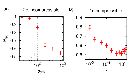
Figure 5: (A) Fixation probability in the two-dimensional incompressible flow of Eq. (31) as a function of the inverse turbulent scale $k$. Parameters are: $\gamma=1$, $\delta D/D=10^{-2}$, $N=10^{4}$, $D=10^{-4}$ and $L=1$. For these parameters, one has $l_{*}\approx 0.01$. (B) Fixation probability in a one-dimensional compressible flow $v=\gamma\sin(2\pi x)$, as a function of the forcing intensity $\gamma$. Parameters are $D=2\cdot 10^{-5}$, $N=10^{3}$, $\delta D/D=0.2$, $f_{0}=1/2$, $L=1$.

Finally, we briefly discuss what happens in the presence of a compressible flow, where species localize near sinks in the velocity field prasad prl_pigolotti . The characteristic localization scale $l_{c}$ near a sink is of order $\sqrt{D/\Gamma}$ where $\Gamma$ is the typical velocity gradient benzi . When $l_{c}$ is smaller than $l_{*}$, the effect due to localization should greatly reduce the effect of having a larger diffusivity. Consequently, we expect a significant decrease in $P_{fix}$ for $\Gamma\sim\sqrt{\mu/t_{f}}$. This scenario is supported by simulations shown in Fig. (5B), where we plot $P_{fix}$ obtained in a $1d$ system subject to a simple compressible flow, $v(x)=\gamma\sin(2\pi x)$, see prl_pigolotti for a comparison with $\delta D=0$. As predicted, we observe a strong decrease of $P_{fix}$ at increasing $\gamma$.

- (1) I. Dornic, H. Chate, J. Chave, and H. Hinrichsen, Phys. Rev. Lett. 87, 045701 (2001).
- (2) M. Kimura and G. H. Weiss, Genetics 49, 561-576 (1964).
- (3) J. F. Crow and M. Kimura An Introduction to Population Genetics, Blackburn Press, Caldwell, NJ (2009).
- (4) O. Hallatschek, P. Hersen, S. Ramanathan, and D. R. Nelson, Proc. Natl. Acad. Sci 104, 19926-19930 (2007).
- (5) K. S. Korolev, M. J. Mueller, N. Karahan, A. W. Murray, O. Hallatschek and D. R. Nelson, Physical Biology 9(2), 026008 (2012).
- (6) R. A. Fisher, Ann. Eugenics 7, 353-369 (1937).
- (7) A. Kolmogorov, N. Petrovsky, and N. Piscounov, Moscow Univ. Math. Bull. 1, 1-25 (1937).
- (8) E. Brunet and B. Derrida, Phys. Rev. E 56, 2597 (1997).
- (9) L. Pechenik and H. Levine, Phys. Rev. E 59, 3893 (1999).
- (10) C. R. Doering, C. Mueller and P. Smereka, Physica A 325(1-2), 243–259 (2003).
- (11) O. Hallatschek and K. S. Korolev, Phys. Rev. Lett. 103, 108103 (2009).
- (12) O. Al Hammal, H. Chate, I. Dornic, M. A. Muñoz, Phys. Rev. Lett. 94, 23601 (2005).
- (13) V. Elgart and A. Kamenev, Phys. Rev. E 74, 041101 (2006).
- (14) O. Hallatschek, PLoS Comput Biol 7(3): e1002005 (2011).
- (15) S. Pigolotti, R. Benzi, P. Perlekar, M.H. Jensen, F. Toschi, and D.R. Nelson, Theo. Pop. Biol. 84, 72-86 (2013).
- (16) C. Gardiner Handbook of Stochastic Methods: for Physics, Chemistry and the Natural Sciences, Springer Series in Synergetics (2004).
- (17) S. Pigolotti, R. Benzi, M.H. Jensen and D. R. Nelson, Phys. Rev. Lett. 108, 128102 (2012).
- (18) For a recent review, see K. Korolev et al. Rev. Mod. Phys. 820, 1691-1718 (2010).
- (19) O. Benichou, V. Calvez, N. Meunier and R. Voituriez, Phys. Rev. E 86, 041908 (2012).
- (20) E. Heinsalu, E. Hernandez-Garcia and C. Lopez, Phys Rev. Lett. 110, 258101 (2013).
- (21) W. D. Hamilton and R. M. May, Nature 269, 578-581 (1977).
- (22) H. N. Comins, W. D. Hamilton, and R. M. May, J. Theo. Biol. 82, 205-230 (1980).
- (23) P. L. Krapivsky, Phys. Rev. A 45, 1067–1072 (1992).
- (24) T. Reichenbach, M. Mobilia, and E. Frey, Nature 448, 1046-1049 (2007).
- (25) N. Fujiwara, J. Kurths and A. Diaz-Guilera, Phys. Rev. E 83, 025101 (2011).
- (26) Supplementary Information accompain this paper.
- (27) Risken H (1996) The Fokker-Planck Equation: Methods of Solution and Applications, Springer-Verlag, Berlin.
- (28) Van Kampen NG (2007), Stochastic Processes in Physics and Chemistry, Elsevier, Amsterdam.
- (29) L. Biferale, A. Crisanti, M. Vergassola, A. Vulpiani, Phys. Fluids 7(11):2725-2734 (1995).
- (30) R. Benzi, D. R. Nelson Physica D 238, 2003-2015 (2009).
- (31) P. Perlekar et al. Phys. Rev. Lett. 105, 144501 (2010).
- (32) Bresnan, E. et al. J. Sea Res., 61(1-2), 17–25 (2009). P. Mariani et al. Limnol. Oceanogr., 58(1), 173–184 (2013).
- (33) R. A. Wheatcroft, P. A. Jumars, C. R. Smith and A. R. M. Nowell, J. Marine Research, 48, 177-207,(1990)
- (34) Miles G. McPhee, J. Phys. Oceanography, 24, 2014-2031, (1994)