Sparse Packetized Predictive Control for Networked Control over Erasure Channels

Abstract

We study feedback control over erasure channels with packet-dropouts. To achieve robustness with respect to packet-dropouts, the controller transmits data packets containing plant input predictions, which minimize a finite horizon cost function. To reduce the data size of packets, we propose to adopt sparsity-promoting optimizations, namely, $\ell^{1}\text{-}\ell^{2}$ and $\ell^{2}$-constrained $\ell^{0}$ optimizations, for which efficient algorithms exist. We show how to design the tuning parameters to ensure (practical) stability of the resulting feedback control systems when the number of consecutive packet-dropouts is bounded.

I Introduction

In networked control systems (NCSs) communication between controller(s) and plant(s) is made through unreliable and rate-limited communication links such as wireless networks and the Internet; see e.g., [1]. Many interesting challenges arise and successful NCS design methods need to consider both control and communication aspects. In particular, so-called packetized predictive control (PPC) has been shown to have favorable stability and performance properties, especially in the presence of packet-dropouts [2, 3, 4]. In PPC, the controller output is obtained through minimizing a finite-horizon cost function on-line and in a receding horizon manner. Each control packet contains a sequence of tentative plant inputs for a finite horizon of future time instants and is transmitted through a communication channel. Packets which are successfully received at the plant actuator side, are stored in a buffer to be used whenever later packets are dropped. When there are no packet-dropouts, PPC reduces to model predictive control. For PPC to give desirable closed-loop properties, the more unreliable the network is, the larger the horizon length (and thus the number of tentative plant input values contained in each packet) needs to be chosen. Clearly, in principle, this would require increasing the network bandwidth (i.e., its bit-rate), unless the transmitted signals are suitably encoded. It is well-known that there exists a minimum bit-rate for achieving stability of a networked feedback control system [5, 1]. The optimal quantizer for the minimum bit-rate is a dynamic vector quantizer, and is, thus, hard to use in many applications. As an alternative, memoryless scalar quantizers, will often be preferable. In this case, sparse representations [6] can be used to reduce the data size of transmitted vectors in PPC. Sparse representations aim at designing sparse vectors, which have few non-zero coefficients, along with optimizing some performance indices. Since sparse vectors contain many zero-valued elements, they can be easily compressed by only encoding a few nonzero coefficients and their locations with a memoryless scalar quantizer. Well-known examples of this kind of encoding are JPEG in image processing [7] and algebraic CELP in speech coding [8, Section 17.11.1]. Over the past few years, a number of studies have been published which deal with sparsity for control, including topics such as trajectory generation [9], state observation [10, 11], optimal control [12, 13, 14, 15, 16, 17, 18], and also sampled-data control [19, 20, 21].

The purpose of the present work is to introduce sparsity-promoting optimizations for networked control with dropouts. We will show that sparsity-promoting cost functions can be used in PPC to achieve good control performance (as measured by a weighted quadratic norm of the system state), whilst transmitting sequences with only few non-zero elements. By studying the sequence of optimal cost functions at the instances of successful reception, we derive sufficient conditions for (practical) closed-loop stability in the presence of bounded packet-dropouts.

It is well-known that sparsity-promoting optimization, which is often described in terms of the so-called $\ell^{0}$ norm [6], is in principle hard to solve due to its combinatorial nature [22]. However, there exist efficient methods that compute the solution (or an approximation) of the optimization in the field of compressed sensing (see e.g., [23]). We will focus on two such methods: One is convex relaxation where the $\ell^{1}$ norm is used in place of the highly nonconvex $\ell^{0}$ norm. This leads to $\ell^{1}\text{-}\ell^{2}$ optimization ($\ell^{1}$-regularized $\ell^{2}$ optimization), which can be effectively solved with a fast algorithm called Fast Iterative Shrinkage-Thresholding Algorithm (FISTA) [24]. The other approach to obtain sparse solutions is through adoption of greedy algorithms. A greedy algorithm iteratively builds up the approximate solution of the $\ell^{0}$-norm optimization by updating the support set one by one. In particular, Orthogonal Matching Pursuit (OMP) [25] is quite simple and known to be dramatically faster than exhaustive search.

Our present note complements our recent conference contribution[26], which adopted an $\ell^{1}\text{-}\ell^{2}$ optimization for PPC. A limitation of the approach in[26] is that for open-loop unstable systems, asymptotic stability cannot be obtained in the presence of bounded packet-dropouts; the best one can hope for is practical stability. Our current paper also complements the articles [27, 28], by presenting a detailed technical analysis of the scheme, including proofs of results.

The remainder of this note is organized as follows: Section II revises basic elements of packetized predictive control. In Section III, we show the motivation of sparsity-promoting optimization for PPC, and formulate the design of the sparse control packets. In Section IV, we study stability of the resultant networked control system. A numerical example is included in Section V. Section VI draws conclusions.

Notation

We write $\mathbb{N}_{0}$ for $\{0,1,2,3,\ldots\}$. The identity matrix (of appropriate dimensions) is denoted via $I$. For a matrix (or a vector) $A$, $A^{\top}$ denotes the transpose. For a vector ${\boldsymbol{v}}=[v_{1},\ldots,v_{n}]^{\top}\in\mathbb{R}^{n}$ and a positive definite matrix $P>0$, we define $\|{\boldsymbol{v}}\|_{1}\triangleq|v_{1}|+\dots+|v_{n}|$, $\|{\boldsymbol{v}}\|_{2}\triangleq\sqrt{{\boldsymbol{v}}^{\top}{\boldsymbol{v}}}$, $\|{\boldsymbol{v}}\|_{P}\triangleq\sqrt{{\boldsymbol{v}}^{\top}P{\boldsymbol{v}}}$, and $\|{\boldsymbol{v}}\|_{\infty}\triangleq\max\{|v_{1}|,\dots,|v_{n}|\}$. The support set $\operatorname*{supp}({\boldsymbol{v}})$ of vector ${\boldsymbol{v}}$ is defined as $\operatorname*{supp}({\boldsymbol{v}})=\{i:v_{i}\neq 0\}$, and the “$\ell^{0}$ norm” of ${\boldsymbol{v}}$ is defined as $\|{\boldsymbol{v}}\|_{0}=|\operatorname*{supp}({\boldsymbol{v}})|$ where $|\cdot|$ denotes the cardinality of a set. Thus, $\|{\boldsymbol{v}}\|_{0}$ is the number of nonzero elements in ${\boldsymbol{v}}$. For any Hermitian matrix $P$, $\lambda_{\max}(P)$ and $\lambda_{\min}(P)$ denote the maximum and the minimum eigenvalues of $P$, respectively; $\sigma_{\max}^{2}(P)\triangleq\lambda_{\max}(P^{\top}P)$.

II Packetized Predictive Networked Control

Let us consider an unconstrained discrete-time linear time-invariant plant model with a scalar input:

$${\boldsymbol{x}}(k+1)=A{\boldsymbol{x}}(k)+Bu(k),\quad k\in\mathbb{N}_{0},\quad{\boldsymbol{x}}(0)={\boldsymbol{x}}_{0}\in\mathbb{R}^{n},$$ (1)

where ${\boldsymbol{x}}(k)\in\mathbb{R}^{n}$, $u(k)\in\mathbb{R}$. Throughout this work, we assume that the pair $(A,B)$ is reachable.

We are interested in an NCS architecture, where the controller communicates with the plant actuator through an erasure channel, as depicted in Fig. 1.

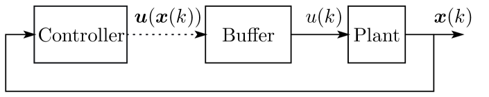
Figure 1: Networked Control System with PPC. The dotted line indicates an erasure channel.

This channel introduces packet-dropouts, which we model via the dropout sequence $\{d(k)\}_{k\in\mathbb{N}_{0}}$ where $d(k)=1$ if packet-dropout occurs and $d(k)=0$ otherwise. With Packetized Predictive Control (PPC), as described, for instance, in [3], at each time instant $k$, the controller uses the state ${\boldsymbol{x}}(k)$ of the plant (1) to calculate and sends a control packet of the form ${\boldsymbol{u}}({\boldsymbol{x}}(k))=[u_{0}({\boldsymbol{x}}(k)),\dots,u_{N-1}({\boldsymbol{x}}(k))]^{\top}\in\mathbb{R}^{N},$ to the plant input node.

To achieve robustness against packet-dropouts, buffering is used. More precisely, suppose that at time instant $k$, we have $d(k)=0$, i.e., the data packet ${\boldsymbol{u}}({\boldsymbol{x}}(k))$ is successfully received at the plant input side. Then, this packet is stored in a buffer, overwriting its previous contents. If the next packet ${\boldsymbol{u}}({\boldsymbol{x}}(k+1))$ is dropped, then the plant input $u(k+1)$ is set to $u_{1}({\boldsymbol{x}}(k))$, the second element of ${\boldsymbol{u}}({\boldsymbol{x}}(k))$. The elements of ${\boldsymbol{u}}({\boldsymbol{x}}(k))$ are then successively used until some packet ${\boldsymbol{u}}({\boldsymbol{x}}(k+\ell))$, $\ell\geq 2$ is successfully received.

Remark 1

It is worth noting that (1) does not include disturbances. Hence, as an alternative to PPC, one could simply transmit the system state to the actuator and, upon successful reception, the actuator could calculate and implement a semi-infinite plant input sequence. In the present work, we focus on situations where the actuator does not have sufficient computational capabilities precluding such an open-loop control scheme. In contrast, the sparse PPC formulations proposed in the present work provide feedback at all instances where no dropouts occur. Our recent results concerning related schemes, see [3, 29], suggest that, in the presence of disturbances, PPC will exhibit favorable robustness properties.

III Design of Sparse Control Packets

In the present section we present two methods for the design of sparse PPC. The purpose is to obtain many zero elements $u_{i}({\boldsymbol{x}}(k))$ in the control packet ${\boldsymbol{u}}({\boldsymbol{x}}(k))$, cf., [17, 18]. The control packet ${\boldsymbol{u}}({\boldsymbol{x}}(k))$ is designed at each time $k$ via a standard model predictive control formulation:

$${\boldsymbol{u}}({\boldsymbol{x}}(k))=\operatorname*{arg\,min}_{{\boldsymbol{u}}\in{\mathcal{U}}({\boldsymbol{x}}(k))}\bigl{\{}F({\boldsymbol{x}}^{\prime}_{N})+\sum_{i=0}^{N-1}L({\boldsymbol{x}}^{\prime}_{i},u_{i})\bigr{\}},$$ (2)

where ${\boldsymbol{x}}^{\prime}_{i}$ and $u_{i}$ are state and input predictions, respectively, defined by ${\boldsymbol{x}}^{\prime}_{0}={\boldsymbol{x}}$, ${\boldsymbol{x}}^{\prime}_{i+1}=A{\boldsymbol{x}}^{\prime}_{i}+Bu_{i}$, and ${\boldsymbol{u}}=[u_{0},u_{1},\dots,u_{N-1}]^{\top}$. The function $F$ defines the terminal cost and $L$, the stage cost. In (2), we have introduced a constraint set ${\mathcal{U}}({\boldsymbol{x}})$, which is assumed to be a closed subset of $\mathbb{R}^{N}$ and allowed to depend on the state observation ${\boldsymbol{x}}$. More details on the choice of ${\mathcal{U}}({\boldsymbol{x}})$ will be given below.

To obtain a sparse control vector ${\boldsymbol{u}}({\boldsymbol{x}}(k))$, we will investigate two types of sparsity-promoting optimizations, namely, unconstrained $\ell^{1}\text{-}\ell^{2}$ optimization and $\ell^{2}$-constrained $\ell^{0}$ optimization.

III-A Unconstrained $\ell^{1}\text{-}\ell^{2}$ optimization

Here, the terminal and stage costs are given by $L({\boldsymbol{x}},u)=\|{\boldsymbol{x}}\|_{Q}^{2}+\mu\left|u\right|$ and $F({\boldsymbol{x}})=\|{\boldsymbol{x}}\|_{P}^{2}$, where $\mu>0$, $P>0$, and $Q>0$, and ${\mathcal{U}}({\boldsymbol{x}})$ is taken as $\mathbb{R}^{N}$ (unconstrained). With the following notation:

$$\begin{split}G&\triangleq\bar{Q}^{1/2}\Phi,~{}H\triangleq-\bar{Q}^{1/2}\Upsilon,~{}\bar{Q}\triangleq\mathrm{diag}\{Q,\ldots,Q,P\},\\ \Phi&\triangleq\begin{bmatrix}B&0&\ldots&0\\ AB&B&\ldots&0\\ \vdots&\vdots&\ddots&\vdots\\ A^{N-1}B&A^{N-2}B&\ldots&B\end{bmatrix},\quad\Upsilon\triangleq\begin{bmatrix}A\\ A^{2}\\ \vdots\\ A^{N}\end{bmatrix},\end{split}$$ (3)

the optimization can be represented by

$$\begin{split}{\boldsymbol{u}}({\boldsymbol{x}})&=\operatorname*{arg\,min}_{{\boldsymbol{u}}\in\mathbb{R}^{N}}J({\boldsymbol{x}},{\boldsymbol{u}})\\ J({\boldsymbol{x}},{\boldsymbol{u}})&\triangleq\|G{\boldsymbol{u}}-H{\boldsymbol{x}}\|_{2}^{2}+\mu\|{\boldsymbol{u}}\|_{1}+\|{\boldsymbol{x}}\|_{Q}^{2}.\end{split}$$ (4)

This (unconstrained) $\ell^{1}\text{-}\ell^{2}$ optimization is known to produce a sparse vector via very efficient algorithms [23]. By simulation, we often obtain much sparser vectors than those produced by the $\ell^{0}$ method described below (see also Section V). However, due to fundamental properties of the $\ell^{1}\text{-}\ell^{2}$ optimization, the state ${\boldsymbol{x}}(k)$ never converges to the origin if the plant (1) is unstable (see Proposition 4 below). Instead, in Theorem 9 we will establish that, if design parameters $P>0$ and $\mu>0$ in (3) and (4) are appropriately chosen, then the state ${\boldsymbol{x}}(k)$ converges into a closed finite set including the origin.

III-B $\ell^{2}$-Constrained $\ell^{0}$ optimization

Here, $F({\boldsymbol{x}})=0$, whereas the stage cost $L$ is given by $L({\boldsymbol{x}},u)=1$ if $u\neq 0$ and $L({\boldsymbol{x}},u)=0$ if $u=0$. The constraint set ${\mathcal{U}}({\boldsymbol{x}})$, used in (2) is taken as

$${\mathcal{U}}({\boldsymbol{x}})\triangleq\bigl{\{}{\boldsymbol{u}}\in\mathbb{R}^{N}:\|{\boldsymbol{x}}^{\prime}_{N}\|_{P}^{2}+\sum_{i=1}^{N-1}\|{\boldsymbol{x}}^{\prime}_{i}\|_{Q}^{2}\leq\|{\boldsymbol{x}}\|_{W}^{2}\bigr{\}},$$ (5)

where ${\boldsymbol{x}}^{\prime}_{1},\dots,{\boldsymbol{x}}^{\prime}_{N}$ are predicted states that depend on ${\boldsymbol{u}}$. We assume $P>0$, $Q>0$, and $W>0$ are chosen such that the set ${\mathcal{U}}({\boldsymbol{x}})$ is non-empty for all ${\boldsymbol{x}}\in\mathbb{R}^{N}$. In terms of the notation (3), the optimization can, thus, be written as

$$\begin{split}{\boldsymbol{u}}({\boldsymbol{x}})&=\operatorname*{arg\,min}_{{\boldsymbol{u}}\in{\mathcal{U}}({\boldsymbol{x}})}\|{\boldsymbol{u}}\|_{0},\\ {\mathcal{U}}({\boldsymbol{x}})&=\{{\boldsymbol{u}}\in\mathbb{R}^{N}:\|G{\boldsymbol{u}}-H{\boldsymbol{x}}\|_{2}^{2}\leq\|{\boldsymbol{x}}\|_{W}^{2}\}.\end{split}$$ (6)

The $\ell^{0}$ optimization (6) is in general extremely difficult to solve since it requires a combinatorial search that explores all possible sparse supports of ${\boldsymbol{u}}\in\mathbb{R}^{N}$. In fact, it has been proven to be NP hard [22], leading to the development of sub-optimal algorithms; see, e.g. [23]. One approach to the combinatorial optimization is an iterative greedy algorithm called Orthogonal Matching Pursuit (OMP) [25].

Remark 2

In [17, 30, 31, 32], sparse control methods for closed loop control without dropouts were studied, in essence, adopting an $\ell^{0}$-constrained (or sparsity-constrained) $\ell^{2}$ optimization:

$${\boldsymbol{u}}({\boldsymbol{x}})=\operatorname*{arg\,min}_{{\boldsymbol{u}}\in{\mathcal{U}}}\|G{\boldsymbol{u}}-H{\boldsymbol{x}}\|_{2}^{2},~{}{\mathcal{U}}=\{{\boldsymbol{u}}\in\mathbb{R}^{N}:\|{\boldsymbol{u}}\|_{0}\leq S\},$$

where $S$ is a positive integer less than $N$. The optimization above may be effectively solved via the CoSaMP algorithm described in [33]. Since the bound $S$ of $\|{\boldsymbol{u}}\|_{0}$ is specified a priori, one can adopt the interleaved single pulse permutation (ISPP) design [8, Section 17.11.1] for effectively encoding the support data of ${\boldsymbol{u}}$. A disadvantage of this approach is the difficulty in estimating a bound $S$ that guarantees stability of the feedback loop. In contrast, in the following section we will show how design parameters in (2) can be chosen to ensure closed loop stability in the presence of bounded dropouts.

IV Stability Analysis of Sparse PPC Loops

In this section, we provide stability results for sparse PPC with $\ell^{1}\text{-}\ell^{2}$ optimization and $\ell^{2}$-constrained $\ell^{0}$ optimization, as presented in Section III. To establish deterministic stability properties, we here impose a bound on the maximum number of successive dropouts as follows:

Assumption 3 (Bounded packet-dropouts)

The number of consecutive packet-dropouts is uniformly bounded by $N-1$. $\square$

In view of the above, the horizon length $N$ in (2) allows one to trade computational complexity of the on-line optimization for robustness with respect to dropouts. Thus, the less reliable the network is, the larger $N$ should be chosen.

IV-A Stability Analysis of $\ell^{1}\text{-}\ell^{2}$ PPC

We here analyze closed-loop stability of $\ell^{1}\text{-}\ell^{2}$ PPC, see (4). Our analysis uses elements of the technique introduced in [3]. A distinguishing aspect of the situation at hand is that, for open-loop unstable plants, even when there are no packet-dropouts, asymptotic stability will not be achieved, despite the fact that the plant-model in (1) is disturbance-free. In fact, we have the following proposition, which is directly proved from an equivalent dual problem of (4) (see [34, Appendix B]).

Proposition 4

Define $\Omega\triangleq\{{\boldsymbol{x}}\in\mathbb{R}^{n}:\|G^{\top}H{\boldsymbol{x}}\|_{\infty}\leq\mu/2\}.$ If ${\boldsymbol{x}}\in\Omega$, then ${\boldsymbol{u}}({\boldsymbol{x}})={\boldsymbol{0}}$. $\square$

It follows that if ${\boldsymbol{x}}(k)\in\Omega$ and there are no dropouts at time $k$, then the control will be $u(k)=0$. That is, the control system (1) behaves as an open-loop system in the set $\Omega$. Hence, asymptotic stability will in general not be achieved, if $A$ has eigenvalues outside the unit circle. This fundamental property is linked to sparsity of the control vector.

By the fact mentioned above, we will next turn our attention to practical stability (i.e., stability of a set) of the associated networked control system. For that purpose, we will analyze the value function

$$V({\boldsymbol{x}})\triangleq\min_{{\boldsymbol{u}}\in\mathbb{R}^{N}}J({\boldsymbol{x}},{\boldsymbol{u}}),$$ (7)

where $J({\boldsymbol{x}},{\boldsymbol{u}})$ is as in (4). First, we find bounds of $V({\boldsymbol{x}})$.

Lemma 5 (Bounds of $V$)

For any ${\boldsymbol{x}}\in\mathbb{R}^{n}$, we have

$$\lambda_{\min}(Q)\|{\boldsymbol{x}}\|_{2}^{2}\leq V({\boldsymbol{x}})\leq\phi(\|{\boldsymbol{x}}\|_{2}),$$

where $\phi(t)\triangleq a_{1}t+(a_{2}+\lambda_{\max}(Q))t^{2}$, $a_{1}\triangleq\mu\sqrt{n}~{}\sigma_{\max}\left(G^{\dagger}H\right)$, $a_{2}\triangleq\lambda_{\max}(W^{\star})$, and the matrices $G^{\dagger}$ and $W^{\star}$ are given by

$$G^{\dagger}\triangleq(G^{\top}G)^{-1}G^{\top},\quad W^{\star}\triangleq H^{\top}(I-GG^{\dagger})H.$$ (8)

Proof:

Applying ${\boldsymbol{u}}^{\star}({\boldsymbol{x}})=G^{\dagger}H{\boldsymbol{x}}$ to the cost in (7) gives

$$\begin{split}&\|(GG^{\dagger}-I)H{\boldsymbol{x}}\|_{2}^{2}+\mu\|G^{\dagger}H{\boldsymbol{x}}\|_{1}+\|{\boldsymbol{x}}\|_{Q}^{2}\\ &~{}\leq\mu\sqrt{n}\sigma_{\max}(G^{\dagger}H)\|{\boldsymbol{x}}\|_{2}+(\lambda_{\max}(W^{\star})+\lambda_{\max}(Q))\|{\boldsymbol{x}}\|_{2}^{2},\end{split}$$

where we used the norm inequality $\|{\boldsymbol{v}}\|_{1}\leq\sqrt{n}\|{\boldsymbol{v}}\|_{2}$ for any ${\boldsymbol{v}}\in\mathbb{R}^{n}$, see [35]. This and the definition of $V({\boldsymbol{x}})$ in (7) provide the upper bound on $V({\boldsymbol{x}})$. To obtain the lower bound, we simply note that by the definition of $J({\boldsymbol{x}},{\boldsymbol{u}})$, we have $\|{\boldsymbol{x}}\|_{Q}^{2}\leq J({\boldsymbol{x}},{\boldsymbol{u}})$ for any ${\boldsymbol{u}}\in\mathbb{R}^{N}$, and hence $\lambda_{\min}(Q)\|{\boldsymbol{x}}\|_{2}^{2}\leq V({\boldsymbol{x}})$. ∎

Remark 6

The least squares solution ${\boldsymbol{u}}^{\star}({\boldsymbol{x}})=G^{\dagger}H{\boldsymbol{x}}$ approximates the optimizer ${\boldsymbol{u}}({\boldsymbol{x}})$ of the $\ell^{1}\text{-}\ell^{2}$ cost in (4) for given plant state ${\boldsymbol{x}}$. Since the following bound holds [36]:

$$\|G^{\top}(G{\boldsymbol{u}}({\boldsymbol{x}})-H{\boldsymbol{x}})\|_{\infty}=\|G^{\top}G({\boldsymbol{u}}({\boldsymbol{x}})-{\boldsymbol{u}}^{\star}({\boldsymbol{x}}))\|_{\infty}\leq\mu/2,$$

the upper bound for $V({\boldsymbol{x}})$ given in Lemma 5 will be tight, if $\mu$ is small. $\square$

Having established the above preliminary results, we introduce the $i$-th iterated mapping ${\boldsymbol{f}}^{i}$ with the optimal vector ${\boldsymbol{u}}({\boldsymbol{x}})=[u_{0}({\boldsymbol{x}}),\dots,u_{N-1}({\boldsymbol{x}})]^{\top}$ defined in (4) through the recursion

$${\boldsymbol{f}}^{i}({\boldsymbol{x}})\triangleq A^{i}{\boldsymbol{x}}+\sum_{l=0}^{i-1}A^{i-1-l}Bu_{l}({\boldsymbol{x}}),\quad i=1,2,\ldots,N.$$

This mapping describes the plant state evolution during periods of consecutive packet-dropouts. Note that, since the input ${\boldsymbol{u}}({\boldsymbol{x}})$ is not a linear function of ${\boldsymbol{x}}$ (see Proposition 4), the function ${\boldsymbol{f}}^{i}({\boldsymbol{x}})$ is nonlinear. The following bound plays a crucial role to establish deterministic stability guarantees:

Lemma 7 (Open-loop bound)

Assume that $P>0$ satisfies the following Riccati equation

$$P=A^{\top}PA-A^{\top}PB(B^{\top}PB+r)^{-1}B^{\top}PA+Q$$ (9)

with $r=\mu^{2}N/(4\epsilon)$, $\epsilon>0$. Then for any ${\boldsymbol{x}}\in\mathbb{R}^{n}$ and $i=1,2,\dots,N$, we have

$$V({\boldsymbol{f}}^{i}({\boldsymbol{x}}))-V({\boldsymbol{x}})\leq-\lambda_{\min}(Q)\|{\boldsymbol{x}}\|_{2}^{2}+\epsilon.$$ (10)

Proof:

Fix $i\in\{1,\ldots,N-1\}$ and consider the sequence

$$\tilde{{\boldsymbol{u}}}=\left\{u_{i}({\boldsymbol{x}}),u_{i+1}({\boldsymbol{x}}),\dots,u_{N-1}({\boldsymbol{x}}),\tilde{u}_{N},\ldots,\tilde{u}_{N+i-1}\right\},$$

where $\tilde{u}_{N+j}$ ($j=0,1,\ldots,i-1$) is given by $\tilde{u}_{N+j}=K\tilde{{\boldsymbol{x}}}_{N+j}$ and $\tilde{{\boldsymbol{x}}}_{N+j+1}=A\tilde{{\boldsymbol{x}}}_{N+j}+B\tilde{u}_{N+j}$, where $K=-(B^{\top}PB+r)^{-1}B^{\top}PA$ and $\tilde{{\boldsymbol{x}}}_{N}={\boldsymbol{f}}^{N}({\boldsymbol{x}})$. We then have

$$\begin{split}J({\boldsymbol{f}}^{i}({\boldsymbol{x}}),\tilde{{\boldsymbol{u}}})&=V({\boldsymbol{x}})-\sum_{l=0}^{i-1}\left\{\|{\boldsymbol{f}}^{l}({\boldsymbol{x}})\|_{Q}^{2}+\mu\left|u_{l}({\boldsymbol{x}})\right|\right\}\\ &~{}+\sum_{l=N}^{N+i-1}\left\{\|\tilde{{\boldsymbol{x}}}_{l+1}\|_{P}^{2}-\|\tilde{{\boldsymbol{x}}}_{l}\|_{P}^{2}+\|\tilde{{\boldsymbol{x}}}_{l}\|_{Q}^{2}+\mu\left|\tilde{u}_{l}({\boldsymbol{x}})\right|\right\}.\end{split}$$

By the relation $\tilde{{\boldsymbol{x}}}_{l+1}=(A+BK)\tilde{{\boldsymbol{x}}}_{l}$ and $\tilde{u}_{l}=K\tilde{{\boldsymbol{x}}}_{l}$ for $l=N,N+1,\ldots,N+i-1$, we can bound the terms in the last sum above by

$$\begin{split}&\|\tilde{{\boldsymbol{x}}}_{l+1}\|_{P}^{2}-\|\tilde{{\boldsymbol{x}}}_{l}\|_{P}^{2}+\|\tilde{{\boldsymbol{x}}}_{l}\|_{Q}^{2}+\mu\left|\tilde{u}_{l}({\boldsymbol{x}})\right|\\ &=\tilde{{\boldsymbol{x}}}_{l}^{\top}\!\left[(A+BK)^{\top}P(A+BK)-P+Q+\frac{\mu^{2}N}{4\epsilon}K^{\top}K\right]\!\tilde{{\boldsymbol{x}}}_{l}\\ &\quad-\frac{\mu^{2}N}{4\epsilon}\left(|K\tilde{{\boldsymbol{x}}}_{l}|-\frac{2\epsilon}{\mu N}\right)^{2}+\frac{\epsilon}{N}\leq\frac{\epsilon}{N}.\end{split}$$

Thus, the cost function $J({\boldsymbol{f}}^{i}({\boldsymbol{x}}),\tilde{{\boldsymbol{u}}})$ can be upper bounded by

$$\begin{split}J({\boldsymbol{f}}^{i}({\boldsymbol{x}}),\tilde{{\boldsymbol{u}}})&\leq V({\boldsymbol{x}})-\lambda_{\min}(Q)\|{\boldsymbol{x}}\|_{2}^{2}+\epsilon,\end{split}$$ (11)

where we have used the relation ${\boldsymbol{f}}^{0}({\boldsymbol{x}})={\boldsymbol{x}}$. Since $V({\boldsymbol{f}}^{i}({\boldsymbol{x}}))$ is the minimal value of $J({\boldsymbol{f}}^{i}({\boldsymbol{x}}),{\boldsymbol{u}})$ among all ${\boldsymbol{u}}$’s in $\mathbb{R}^{N}$, we have $V({\boldsymbol{f}}^{i}({\boldsymbol{x}}))\leq J({\boldsymbol{f}}^{i}({\boldsymbol{x}}),\tilde{{\boldsymbol{u}}})$ , and hence inequality (10) holds. For the case $i=N$, we consider the sequence $\tilde{{\boldsymbol{u}}}=\left\{\tilde{u}_{N},\tilde{u}_{N+1},\ldots,\tilde{u}_{2N-1}\right\}$. If we define $\sum_{l=N}^{N-1}=0$, then (11) follows as in the case $i\leq N-1$. ∎

The above result can be used to derive the following contraction property of the optimal costs during periods of successive packet-dropouts:

Lemma 8 (Contractions)

Let $\epsilon>0$. Assume that $P>0$ satisfies (9) with $r=\mu^{2}N/(4\epsilon)$. Then there exists a real number $\rho\in(0,1)$ such that for all ${\boldsymbol{x}}\in\mathbb{R}^{n}$, we have

$$V({\boldsymbol{f}}^{i}({\boldsymbol{x}}))\leq\rho V({\boldsymbol{x}})+\epsilon+\lambda_{\min}(Q)/4,\quad i=1,2,\ldots,N.$$

Proof:

In this proof, we borrow a technique used in the proof of [37, Theorem 4.2.5]. By Lemma 5, for ${\boldsymbol{x}}\neq{\boldsymbol{0}}$ we have

$$0<V({\boldsymbol{x}})\leq a_{1}\|{\boldsymbol{x}}\|_{2}+(a_{2}+\lambda_{\max}(Q))\|{\boldsymbol{x}}\|_{2}^{2}.$$

Now suppose that $0<\|{\boldsymbol{x}}\|_{2}\leq 1$. Then $\|{\boldsymbol{x}}\|_{2}^{2}\leq\|{\boldsymbol{x}}\|_{2}$ and hence $V({\boldsymbol{x}})\leq(a_{1}+a_{2}+\lambda_{\max}(Q))\|{\boldsymbol{x}}\|_{2}$. From Lemma 7, it follows that

$$\begin{split}V({\boldsymbol{f}}^{i}({\boldsymbol{x}}))&\leq(1-\lambda_{\min}(Q)\|{\boldsymbol{x}}\|_{2}V({\boldsymbol{x}})^{-1})V({\boldsymbol{x}})\\ &\qquad-\!\lambda_{\min}(Q)\!\left(\|{\boldsymbol{x}}\|^{2}_{2}-\|{\boldsymbol{x}}\|_{2}\right)+\epsilon\\ &\leq\rho V({\boldsymbol{x}})+\lambda_{\min}(Q)/4+\epsilon,\end{split}$$

with

$$\rho\triangleq 1-\lambda_{\min}(Q)(a_{1}+a_{2}+\lambda_{\max}(Q))^{-1}.$$ (12)

Since $0<\lambda_{\min}(Q)\leq\lambda_{\max}(Q)$, $a_{1}>0$, and $a_{2}>0$, it follows that $\rho\in(0,1)$.

Next, consider the case where $\|{\boldsymbol{x}}\|_{2}>1$ so that $\|{\boldsymbol{x}}\|_{2}<\|{\boldsymbol{x}}\|_{2}^{2}$ and $V({\boldsymbol{x}})<(a_{1}+a_{2}+\lambda_{\max}(Q))\|{\boldsymbol{x}}\|_{2}^{2}$. This and Lemma 7 give

$$\begin{split}V({\boldsymbol{f}}^{i}({\boldsymbol{x}}))&<\rho V({\boldsymbol{x}})+\epsilon\leq\rho V({\boldsymbol{x}})+\lambda_{\min}(Q)/4+\epsilon.\end{split}$$

If ${\boldsymbol{x}}={\boldsymbol{0}}$, then the above inequality also holds since $V({\boldsymbol{0}})={\boldsymbol{0}}$. ∎

We will next use Lemma 8 to establish sufficient conditions for practical stability of $\ell^{1}\text{-}\ell^{2}$ PPC in the presence of packet-dropouts. Theorem 9 stated below shows how to design the parameters of the cost function to ensure practical stability in the presence of bounded packet-dropouts satisfying Assumption 3.

Theorem 9 (Practical stability of $\ell^{1}$-$\ell^{2}$ PPC)

Let $\epsilon>0$ and choose $P>0$ to satisfy (9) with $r=\mu^{2}N/(4\epsilon)$. Then $\|{\boldsymbol{x}}(k)\|_{2}$ is bounded for all $k\in\mathbb{N}_{0}$, and

$$\lim_{k\rightarrow\infty}\|{\boldsymbol{x}}(k)\|_{2}\leq R\triangleq\sqrt{\frac{1}{1-\rho}\left(\frac{\epsilon}{\lambda_{\min}(Q)}+\frac{1}{4}\right)},$$ (13)

where $\rho$ is given in (12).

Proof:

Denote the time instants where there are no packet-dropouts, i.e., where $d(k)=0$, as

$$\mathcal{K}\triangleq\{k_{i}\}_{i\in\mathbb{N}_{0}}\subseteq\mathbb{N}_{0},\quad k_{i+1}>k_{i},\;\forall i\in\mathbb{N}_{0},$$ (14)

whereas the number of consecutive packet-dropouts is denoted via:

$$m_{i}\triangleq k_{i+1}-k_{i}-1,\quad i\in\mathbb{N}_{0}.$$ (15)

Note that $m_{i}\geq 0$, with equality if and only if no dropouts occur between instants $k_{i}$ and $k_{i+1}$. Fix $i\in\mathbb{N}_{0}$ and note that at time instant $k_{i}$, the control packet is successfully transmitted to the buffer. Then until the next packet is received at time $k_{i+1}$, $m_{i}$ consecutive packet-dropouts occur. By the PPC strategy, the control input becomes $u(k_{i}+l)=u_{l}({\boldsymbol{x}}(k_{i}))$, $l=1,2,\ldots,m_{i}$, and, since (1) is exact, the states ${\boldsymbol{x}}(k_{i}+1),\ldots,{\boldsymbol{x}}(k_{i}+m_{i})$ are determined by these open-loop controls. Since we have $m_{i}\leq N-1$ from Assumption 3, Lemma 8 gives

$$V({\boldsymbol{x}}(k))\leq\rho V({\boldsymbol{x}}(k_{i}))+\epsilon+\lambda_{\min}(Q)/4,$$ (16)

for $k\in\{k_{i}+1,k_{i}+2,\ldots,k_{i}+m_{i}\}$, and also for $k_{i+1}=k_{i}+m_{i}+1$, we have

$$V({\boldsymbol{x}}(k_{i+1}))\leq\rho V({\boldsymbol{x}}(k_{i}))+\epsilon+\lambda_{\min}(Q)/4.$$ (17)

Now by induction from (17), it is easy to see that from Lemma 5,

$$\begin{split}V({\boldsymbol{x}}(k_{i}))&\leq\rho^{i}V({\boldsymbol{x}}(k_{0}))+(1+\cdots+\rho^{i-1})(\epsilon+\lambda_{\min}(Q)/4)\\ &\leq\rho^{i}\phi(\|{\boldsymbol{x}}(k_{0})\|_{2})+(1-\rho)^{-1}(\epsilon+\lambda_{\min}(Q)/4).\end{split}$$

This inequality and (16) give the bound

$$\begin{split}V({\boldsymbol{x}}(k))&\leq\rho^{i+1}\phi(\|{\boldsymbol{x}}(k_{0})\|_{2})+(1-\rho)^{-1}(\epsilon+\lambda_{\min}(Q)/4),\\ \end{split}$$

for $k\in\{k_{i}+1,k_{i}+2,\ldots,k_{i+1}-1\}$, and this inequality also holds for $k=k_{i+1}$. Finally, by using the lower bound of $V({\boldsymbol{x}})$ provided in Lemma 5, we have

$$\begin{split}\|{\boldsymbol{x}}(k)\|_{2}&\leq\sqrt{\frac{V({\boldsymbol{x}}(k))}{\lambda_{\min}(Q)}}\leq(\sqrt{\rho})^{i+1}\sqrt{\frac{\phi(\|{\boldsymbol{x}}(k_{0})\|_{2})}{\lambda_{\min}(Q)}}+R,\\ \end{split}$$

where $R$ is defined in (13) and we used the inequality $\sqrt{a+b}\leq\sqrt{a}+\sqrt{b}$, for all $a,b\geq 0$. The above inequality leads to (13). ∎

Theorem 9 establishes practical stability of the networked control system. It shows that, provided the conditions are met, the plant state will be ultimately bounded in a ball of radius $R$. It is worth noting that, as in other stability results which use Lyapunov techniques, this bound will, in general, not be tight.

IV-B Stability Analysis of $\ell^{0}$ PPC

Here we analyze closed-loop stability of $\ell^{0}$ PPC, as described in (6). Since stability will unavoidably be linked to feasibility, we begin with analysis of the feasible set ${\mathcal{U}}({\boldsymbol{x}})$ given in (5). Clearly, for given matrices $G$ and $H$, the feasible set ${\mathcal{U}}({\boldsymbol{x}})$ will be non-empty if the matrix $W$ is “larger” than $W^{\star}$ given in (8), the “smallest” $W$ which ensures that ${\mathcal{U}}({\boldsymbol{x}})\not=\emptyset$. In fact, we have:

Lemma 10

Let

$${\mathcal{U}}^{\star}({\boldsymbol{x}})\triangleq\{{\boldsymbol{u}}\in\mathbb{R}^{N}:\|G{\boldsymbol{u}}-H{\boldsymbol{x}}\|_{2}^{2}\leq\|{\boldsymbol{x}}\|_{W^{\star}}^{2}\}.$$

For any $W\geq W^{\star}$, we have ${\mathcal{U}}({\boldsymbol{x}})\supseteq{\mathcal{U}}^{\star}({\boldsymbol{x}})$. Moreover, if $W\geq W^{\star}$, then the feasible set ${\mathcal{U}}({\boldsymbol{x}})$ is a closed, convex, and non-empty subset of $\mathbb{R}^{N}$.

Proof:

Suppose $W\geq W^{\star}$. Then ${\boldsymbol{u}}^{\star}({\boldsymbol{x}})\in{\mathcal{U}}({\boldsymbol{x}})$ and hence ${\mathcal{U}}({\boldsymbol{x}})\supseteq{\mathcal{U}}^{\star}({\boldsymbol{x}})$. This also implies that ${\mathcal{U}}({\boldsymbol{x}})$ is non-empty for any $W\geq W^{\star}$. Closedness and convexity of ${\mathcal{U}}({\boldsymbol{x}})$ are obvious since it is defined by a quadratic form (the set is a closed ellipsoid in $\mathbb{R}^{N}$). ∎

Based on this lemma, we hereafter assume that

$${\mathcal{E}}\triangleq W-W^{\star}>0.$$ (18)

The feasible solutions for (6) can be characterized as follows:

Lemma 11 (Feasible Solutions)

For any ${\boldsymbol{u}}\in{\mathcal{U}}({\boldsymbol{x}})$, there exists ${\boldsymbol{\varepsilon}}({\boldsymbol{x}})\in\mathbb{R}^{N}$ such that

$${\boldsymbol{u}}={\boldsymbol{u}}^{\star}({\boldsymbol{x}})+{\boldsymbol{\varepsilon}}({\boldsymbol{x}}),~{}\text{with}\quad\|G{\boldsymbol{\varepsilon}}({\boldsymbol{x}})\|^{2}_{2}\leq\|{\boldsymbol{x}}\|_{\mathcal{E}}^{2},$$ (19)

where ${\mathcal{E}}$ is given in (18).

Proof:

The fact $G{\boldsymbol{\varepsilon}}({\boldsymbol{x}})\perp(G{\boldsymbol{u}}^{\star}({\boldsymbol{x}})-H{\boldsymbol{x}})$ gives the result. ∎

Remark 12

The error term ${\boldsymbol{\varepsilon}}({\boldsymbol{x}})$ in (19) may be interpreted as a “penalty charge” for sparsifying the vector (control packet) ${\boldsymbol{u}}$, since the term $\|G{\boldsymbol{u}}({\boldsymbol{x}})-H{\boldsymbol{x}}\|_{2}^{2}$ with the sparse control ${\boldsymbol{u}}({\boldsymbol{x}})$ will be larger than with the least squares one, $\|G{\boldsymbol{u}}^{\star}({\boldsymbol{x}})-H{\boldsymbol{x}}\|_{2}^{2}$. $\square$

Now take $Q>0$ arbitrarily and let $P>0$ be the solution to the Riccati equation (9) with $r=0$. Then, from Lemma 11 and well-known results in dynamic programming [38, Chapter 3], all feasible control vectors ${\boldsymbol{u}}({\boldsymbol{x}})\in{\mathcal{U}}({\boldsymbol{x}})$ can be written as

$$u_{i}({\boldsymbol{x}})=K(A+BK)^{i}{\boldsymbol{x}}+\varepsilon_{i}({\boldsymbol{x}}),\quad i=0,1,\ldots,N-1,$$

where

$$K\triangleq-(B^{\top}PB)^{-1}B^{\top}PA,$$ (20)

and $\varepsilon_{i}({\boldsymbol{x}})$ is the $(i+1)$-th element of ${\boldsymbol{\varepsilon}}({\boldsymbol{x}})$ satisfying the inequality in (19). The associated open-loop states are

$${\boldsymbol{x}}_{0}={\boldsymbol{x}},\quad{\boldsymbol{x}}_{i+1}=(A+BK){\boldsymbol{x}}_{i}+Bw_{i}({\boldsymbol{x}}),$$ (21)

where

$$w_{i}({\boldsymbol{x}})\triangleq\varepsilon_{i}({\boldsymbol{x}})-K\sum_{l=0}^{i-1}A^{i-1-l}B\varepsilon_{l}({\boldsymbol{x}}).$$ (22)

By using the definition (20) of the matrix $K$, we have

$$w_{i}({\boldsymbol{x}})=(B^{\top}PB)^{-1}B^{\top}P\Phi_{i}{\boldsymbol{\varepsilon}}({\boldsymbol{x}}),\quad i=0,1,\ldots,N-1,$$

where $\Phi_{i}\in\mathbb{R}^{n\times N}$ is the $(i+1)$-th row block of the matrix $\Phi$ defined in (3).

For the $\ell_{0}$-case, we use the quadratic function $V_{P}({\boldsymbol{x}})\triangleq\|{\boldsymbol{x}}\|_{P}^{2}$ as a Lyapunov function candidate for the system at the times of successful transmission instants. The following result bears some similarities to Lemma 8, with the important difference that in (23) the upper bound goes to zero as ${\boldsymbol{x}}$ goes to the origin.

Lemma 13 (Contractions)

Suppose $Q>0$ is chosen arbitrarily, $P>0$ is the solution of the Riccati equation (9) with $r=0$, and $W>0$ is such that $W>W^{\star}$. Let ${\mathcal{E}}=W-W^{\star}$. Then there exist constants $\rho\in[0,1)$ and $c>0$ such that

$$V_{P}({\boldsymbol{x}}_{i})\leq\rho^{i}V_{P}({\boldsymbol{x}})+c\|{\boldsymbol{x}}\|_{{\mathcal{E}}}^{2},\quad i=1,2,\ldots,N.$$ (23)

Proof:

Substitution of the state ${\boldsymbol{x}}_{i+1}$ given in (21) into $V_{P}({\boldsymbol{x}})$ yields that

$$V_{P}({\boldsymbol{x}}_{i+1})=V_{P}({\boldsymbol{x}}_{i})-\|{\boldsymbol{x}}_{i}\|_{Q}^{2}+B^{\top}PB\left|w_{i}({\boldsymbol{x}})\right|^{2}.$$

By the definition of $w_{i}({\boldsymbol{x}})$ in (22), we have

$$\begin{split}(B^{\top}PB)&\left|w_{i}({\boldsymbol{x}})\right|^{2}\leq{\boldsymbol{\varepsilon}}({\boldsymbol{x}})\Phi_{i}^{\top}P\Phi_{i}{\boldsymbol{\varepsilon}}({\boldsymbol{x}})\\ &\leq\max_{i}\lambda_{\max}\bigl{\{}\Phi_{i}^{\top}P\Phi_{i}(G^{\top}G)^{-1}\bigr{\}}\|G{\boldsymbol{\varepsilon}}({\boldsymbol{x}})\|_{2}^{2}\leq c_{1}\|{\boldsymbol{x}}\|_{{\mathcal{E}}}^{2},\end{split}$$

where the last inequality is due to Lemma 11, and

$$c_{1}\triangleq\max_{i=0,\ldots,N-1}\lambda_{\max}\bigl{\{}\Phi_{i}^{\top}P\Phi_{i}(G^{\top}G)^{-1}\bigr{\}}>0.$$ (24)

Then the above inequality gives

$$V_{P}({\boldsymbol{x}}_{i+1}) \leq(1-\|{\boldsymbol{x}}_{i}\|_{Q}^{2}\|{\boldsymbol{x}}_{i}\|_{P}^{-2})V_{P}({\boldsymbol{x}}_{i})+c_{1}\|{\boldsymbol{x}}\|_{{\mathcal{E}}}^{2}$$

$$\leq\rho V_{P}({\boldsymbol{x}}_{i})+c_{1}\|{\boldsymbol{x}}\|_{{\mathcal{E}}}^{2},\quad\rho\triangleq 1-\lambda_{\min}(QP^{-1}).$$ (25)

Since $P\geq Q>0$, we have $\rho\in[0,1)$. By mathematical induction, we finally obtain

$$V_{P}({\boldsymbol{x}}_{i}) \leq\rho^{i}V_{P}({\boldsymbol{x}})+(\rho^{i-1}+\cdots+\rho+1)c_{1}\|{\boldsymbol{x}}\|_{{\mathcal{E}}}^{2}$$

$$\leq\rho^{i}V_{P}({\boldsymbol{x}})+c\|{\boldsymbol{x}}\|_{{\mathcal{E}}}^{2},$$ (26)

where $\quad c\triangleq(1-\rho)^{-1}(1-\rho^{N})c_{1}$. ∎

Having established the contraction property (23), the following result shows that $\ell^{0}$-PPC can be tuned to give asymptotic stability in the presence of bounded packet-dropouts:

Theorem 14 (Asymptotic Stability)

Suppose that the matrices $P$, $Q$, and $W$ are chosen by the following procedure:

1. Choose $Q>0$ arbitrarily.

2. Solve the Riccati equation (9) with $r=0$ to obtain $P>0$.

3. Compute $\rho\in[0,1)$ and $c>0$ via (24), (25), and (26).

4. Choose ${\mathcal{E}}$ such that $0<{\mathcal{E}}<(1-\rho)P/c$.

5. Compute $W^{\star}=P-Q$ and set $W=W^{\star}+{\mathcal{E}}$.

Then the sparse control packets ${\boldsymbol{u}}({\boldsymbol{x}}(k))$, $k\in\mathbb{N}_{0}$, optimizing (6) with the above matrices, lead to asymptotic stability of the networked control system, that is, ${\boldsymbol{x}}(k)\rightarrow{\boldsymbol{0}}$ as $k\rightarrow\infty$.

Proof:

We use the notation of time instants where there are no packet-dropouts given in (14) and (15). Fix $i\in\mathbb{N}_{0}$. Since we have $m_{i}\leq N-1$ from Assumption 3, Lemma 13 gives

$$V_{P}({\boldsymbol{x}}(k))\leq{\boldsymbol{x}}(k_{i})^{\top}\left(\rho P+c{\mathcal{E}}\right){\boldsymbol{x}}(k_{i})<V_{P}({\boldsymbol{x}}(k_{i})),$$ (27)

for $k=k_{i},k_{i}+1,\ldots,k_{i}+m_{i}$. Also, for $k_{i+1}=k_{i}+m_{i}+1$, the next instant when the control packet is successfully transmitted, we have

$$V_{P}({\boldsymbol{x}}(k_{i+1}))<V_{P}({\boldsymbol{x}}(k_{i+1}-1))<V_{P}({\boldsymbol{x}}(k_{i})).$$

It follows that at the time instants $k_{0},k_{1},\ldots$ (no-dropout instants), $0\leq V_{P}({\boldsymbol{x}}(k_{i}))$ strictly decreases, and hence ${\boldsymbol{x}}(k_{i})\rightarrow{\boldsymbol{0}}$ as $i\rightarrow\infty$. Then, by (27), for $k=k_{i},k_{i}+1,\ldots,k_{i}+m_{i}$ (consecutive dropout instants), $V_{P}({\boldsymbol{x}}(k))$ is bounded by $V_{P}({\boldsymbol{x}}(k_{i}))$. Since the latter converges to zero, we conclude that ${\boldsymbol{x}}(k)\rightarrow{\boldsymbol{0}}$ as $k\rightarrow\infty$. ∎

In summary, the networked control system affected by bounded packet-dropouts is asymptotically stable with the sparse control packets obtained by the optimization (6) if $P$, $Q$, and $W$ are computed as per Theorem 14.

V Simulation Study

To assess the effectiveness of the proposed sparse control methods, we consider a plant model of the form (1) with

$$A=\left[\begin{array}[]{rrrr}\!\!0.0685&\!\!1.1221&\!\!-0.6615&\!\!0.3087\!\!\\ \!\!0.9512&\!\!0.3237&\!\!-0.2253&\!\!-0.5701\!\!\\ \!\!-0.3448&\!\!-0.4112&\!\!-0.8299&\!\!0.5388\!\!\\ \!\!0.0359&\!\!-0.6418&\!\!-0.1262&\!\!0.4669\!\!\\ \end{array}\right],~{}B=\left[\begin{array}[]{r}\!\!2.3459\!\!\\ \!\!0.0893\!\!\\ \!\!2.2103\!\!\\ \!\!0.7440\!\!\\ \end{array}\right].$$

We set $N=10$ and packet-dropouts are simulated with a model where the probability distribution of the number of consecutive dropouts is uniform over $[1,\dots,N-1]$. For the system above, we make simulation-based examination of the proposed stabilizing PPC formulations using sparsity-promoting optimizations, $\ell^{1}\text{-}\ell^{2}$ optimization with FISTA and $\ell^{0}$ optimization with OMP. We set the horizon length (or the packet size) to $N=10$.

To compare these two sparsity-promoting methods with traditional PPC approaches, we also consider the $\ell^{2}$-optimal control

$${\boldsymbol{u}}_{r}^{\star}({\boldsymbol{x}})=(G^{\top}G+rI)^{-1}G^{\top}{\boldsymbol{x}},$$

that minimizes $\|G{\boldsymbol{u}}-H{\boldsymbol{x}}\|_{2}^{2}+r\|{\boldsymbol{u}}\|_{2}^{2}$, and the ideal least squares solution, namely, ${\boldsymbol{u}}^{\star}({\boldsymbol{x}})=G^{\dagger}H{\boldsymbol{x}}.$

The regularization parameters $\mu$ for the $\ell^{1}\text{-}\ell^{2}$ optimization and $r$ for the $\ell^{2}$ optimization are empirically chosen such that the $\ell^{2}$ norm of the state $\{{\boldsymbol{x}}(k)\}_{k=0}^{99}$ is minimized ($r=4.1042$ and $\mu=10.7167$). For the $\ell^{0}$ optimization, we choose the weighting matrix $Q$ in (6) as $Q=I$, and choose the matrix $W$ according to the procedure shown in Theorem 14 with ${\mathcal{E}}=\frac{2}{3}(1-\rho)P/c<(1-\rho)P/c$.

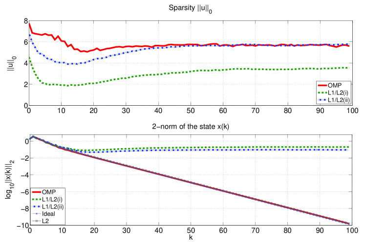
Figure 2: Averaged sparsity $\|{\boldsymbol{u}}({\boldsymbol{x}}(k))\|_{0}$ of the control vectors (top) and averaged 2-norm of the state ${\boldsymbol{x}}(k)$ (bottom).

With these parameters, we run 500 simulations with randomly generated packet-dropouts as described above, and with initial vector ${\boldsymbol{x}}_{0}$ in which each element is independently sampled from the normal distribution with mean 0 and variance 1. The top figure in Fig. 2 shows the averaged sparsity of the obtained control vectors. The $\ell^{1}\text{-}\ell^{2}$ optimization with $\mu=10.7167$, labeled by L1/L2 (i), always produces sparser control vectors than OMP. Clearly, this property depends on how the regularization parameter $\mu>0$ is chosen. In fact, if we choose the smaller value, $\mu=3.3$, then the sparsity approximates that of OMP, as the curve labeled by L1/L2 (ii) in Fig. 2. On the other hand, if we use a sufficiently large $\mu>0$, then the control vector becomes ${\boldsymbol{0}}$. This is indeed the sparsest control, but leads to very poor control performance: the state diverges until the control vector becomes nonzero (in accordance with the stability results established in Section IV). The bottom figure in Fig. 2 shows the averaged 2-norm of the state ${\boldsymbol{x}}(k)$ as a function of $k$ for all 5 designs.

We see that, with exception of the $\ell^{1}\text{-}\ell^{2}$ optimization based PPC, the NCSs are all asymptotically stable. (Our simulation results even suggest exponential stability.) In contrast, if the $\ell^{1}\text{-}\ell^{2}$ optimization of[26] is used, then only practical stability is observed. Note that the $\ell^{1}\text{-}\ell^{2}$ optimization with $\mu=3.3$ has almost the same sparsity as OMP, but the response does not show asymptotic stability while OMP does. The simulation results are consistent with Theorem 9 and Theorem 14.

VI Conclusions

We have studied packetized predictive control formulations with sparsity-promoting cost functions (i.e., $\ell^{1}\text{-}\ell^{2}$ and $\ell^{2}$-constrained $\ell^{0}$ optimizations) for networked control systems with packet dropouts. We have established sufficient conditions for practical stability of $\ell^{1}\text{-}\ell^{2}$-optimal PPC and for asymptotic stability of $\ell^{2}$-constrained $\ell^{0}$-optimal PPC, when the number of successive packet dropouts is bounded. Simulation results indicate that the proposed controllers provide, not only stabilizing but also sparse control packets.

Future work may include obtaining analytical bounds on the sparsity of solutions. It is also of interest to apply the proposed control methods to constrained nonlinear plant models with disturbances, and to channels with bit-rate limitations and unbounded packet-dropouts. We foresee that this will require extending results in[29, 4] and also the development of fast algorithms to solve the associated optimization problems.

References

• [1] G. N. Nair, F. Fagnani, S. Zampieri, and R. J. Evans, “Feedback control under data rate constraints: An overview,” Proc. IEEE, vol. 95, pp. 108–137, Jan. 2007.
• [2] A. Bemporad, “Predictive control of teleoperated constrained systems with unbounded communication delays,” Proc. 37th IEEE CDC, pp. 2133–2138, 1998.
• [3] D. E. Quevedo and D. Nešić, “Input-to-state stability of packetized predictive control over unreliable networks affected by packet-dropouts,” IEEE Trans. Autom. Control, vol. 56, no. 2, pp. 370–375, Feb. 2011.
• [4] D. E. Quevedo, J. Østergaard, and D. Nešić, “Packetized predictive control of stochastic systems over bit-rate limited channels with packet loss,” IEEE Trans. Autom. Control, vol. 56, no. 11, 2011.
• [5] S. Tatikonda and S. Mitter, “Control under communication constraints,” IEEE Trans. Autom. Control, vol. 49, no. 7, pp. 1056–1068, Jul. 2004.
• [6] M. Elad, Sparse and Redundant Representations.   Springer, 2010.
• [7] G. K. Wallace, “The JPEG still picture compression standard,” Commun. ACM, vol. 34, no. 4, pp. 30–44, Apr. 1991.
• [8] J. Benesty, M. M. Sondhi, and Y. Huang, Springer Handbook of Speech Processing.   Springer, 2008.
• [9] H. Ohlsson, F. Gustafsson, L. Ljung, and S. Boyd, “Trajectory generation using sum-of-norms regularization,” in Proc. 49th IEEE CDC, Dec. 2010, pp. 540–545.
• [10] M. Wakin, B. Sanandaji, and T. Vincent, “On the observability of linear systems from random, compressive measurements,” in Proc. 49th IEEE CDC, Dec. 2010, pp. 4447–4454.
• [11] S. Bhattacharya and T. Başar, “Sparsity based feedback design: a new paradigm in opportunistic sensing,” in Proc. Amer. Contr. Conf., Jun.–Jul. 2011, pp. 3704–3709.
• [12] O. I. Kostyukova, E. A. Kostina, and N. M. Fedortsova, “Parametric optimal control problems with weighted $l_{1}$-norm in the cost function,” Automatic Control and Computer Sciences, vol. 44, no. 4, pp. 179–190, 2010.
• [13] S. Schuler, C. Ebenbauer, and F. Allgöwer, “$\ell_{0}$-system gain and $\ell_{1}$-optimal control,” in IFAC 18th World Congress, Aug.–Sept. 2011, pp. 9230–9235.
• [14] M. Fardad, L. Fu, and M. R. Jovanovic, “Sparsity-promoting optimal control for a class of distributed systems,” in Proc. Amer. Contr. Conf., Jun.–Jul. 2011, pp. 2050–2055.
• [15] L. Mathelin, L. Pastur, and L. Maitre, “A compressed-sensing approach for closed-loop optimal control of nonlinear systems,” Theoretical and computational fluid dynamics, vol. 26, no. 1-4, pp. 319–337, 2012.
• [16] M. Gallieri and J. M. Maciejowski, “$\ell_{\rm asso}$ MPC: Smart regulation of over-actuated systems,” in Proc. Amer. Contr. Conf., Jun. 2012, pp. 1217–1222.
• [17] G. Goodwin, H. Haimovich, D. Quevedo, and J. Welsh, “A moving horizon approach to networked control system design,” IEEE Trans. Autom. Control, vol. 49, no. 9, pp. 1427–1445, Sep. 2004.
• [18] D. E. Quevedo, E. I. Silva, and D. Nešić, “Design of multiple actuator-link control systems with packet dropouts,” in Proc. IFAC World Congr., Seoul, Korea, July 2008, pp. 6642–6647.
• [19] M. Nagahara, D. E. Quevedo, J. Østergaard, T. Matsuda, and K. Hayashi, “Sparse command generator for remote control,” in 9th IEEE International Conf.  Control and Automation, Dec. 2011, pp. 1055–1059.
• [20] M. Nagahara, D. E. Quevedo, T. Matsuda, and K. Hayashi, “Compressive sampling for networked feedback control,” in Proc. IEEE ICASSP, Mar. 2012, pp. 2733–2736.
• [21] M. Nagahara, T. Matsuda, and K. Hayashi, “Compressive sampling for remote control systems,” IEICE Trans. on Fundamentals, vol. E95-A, no. 4, pp. 713–722, Apr. 2012.
• [22] B. K. Natarajan, “Sparse approximate solutions to linear systems,” SIAM J. Comput., vol. 24, no. 2, pp. 227–234, 1995.
• [23] K. Hayashi, M. Nagahara, and T. Tanaka, “A user’s guide to compressed sensing for communications systems,” IEICE Trans. on Communications, vol. E96-B, no. 3, pp. 685–712, Mar. 2013.
• [24] A. Beck and M. Teboulle, “A fast iterative shrinkage-thresholding algorithm for linear inverse problems,” SIAM J. Imaging Sci., vol. 2, no. 1, pp. 183–202, Jan. 2009.
• [25] Y. C. Pati, R. Rezaiifar, and P. S. Krishnaprasad, “Orthogonal matching pursuit: Recursive function approximation with applications to wavelet decomposition,” in Proc.  the 27th Annual Asilomar Conf. on Signals, Systems and Computers, Nov. 1993, pp. 40–44.
• [26] M. Nagahara and D. E. Quevedo, “Sparse representations for packetized predictive networked control,” in IFAC 18th World Congress, Aug.–Sept. 2011, pp. 84–89.
• [27] M. Nagahara, D. E. Quevedo, and J. Østergaard, “Sparsely-packetized predictive control by orthogonal matching pursuit (extended abstract),” in 20th International Symposium on Mathematical Theory of Networks and Systems (MTNS), Jul. 2012.
• [28] ——, “Packetized predictive control for rate-limited networks via sparse representation,” in Proc. 51st IEEE CDC, Dec. 2012, pp. 1362–1367.
• [29] D. E. Quevedo and D. Nešić, “Robust stability of packetized predictive control of nonlinear systems with disturbances and Markovian packet dropouts,” Automatica, vol. 48, no. 8, pp. 1803–1811, Aug. 2012.
• [30] O. Imer and T. Başar, “Optimal control with limited controls,” in Proc. Amer. Contr. Conf., 2006, pp. 298–303.
• [31] N. D. Shemonski, “Limiting controls in vector state space systems,” Master Thesis, University of Illinois at Urbana-Champaign, 2012.
• [32] L. Shi, Y. Yuan, and J. Chen, “Finite horizon LQR control with limited controller-system communication,” IEEE Trans. Autom. Control, vol. 58, no. 7, pp. 1835–1841, Jul. 2013.
• [33] D. Needell and J. A. Tropp, “CoSaMP: iterative signal recovery from incomplete and inaccurate samples,” Appl. Comput. Harmonic Anal., vol. 26, no. 3, pp. 301–321, 2008.
• [34] J.-J. Fuchs, “On the application of the global matched filter to DOA estimation with uniform circular arrays,” IEEE Trans. Signal Process., vol. 49, no. 4, pp. 702–709, 2001.
• [35] D. S. Bernstein, Matrix Mathematics.   Princeton University Press, 2009.
• [36] J.-J. Fuchs, “On sparse representations in arbitrary redundant bases,” IEEE Trans. Inf. Theory, vol. 50, no. 6, pp. 1341–11 344, Jun. 2004.
• [37] M. Lazar, “Predictive control algorithms for nonlinear systems,” Doctoral Thesis, Technical University of Iasi, Romana, 2009.
• [38] D. P. Bertsekas, Dynamic Programming and Stochastic Control.   Academic Press, 1976.