On Finding a Subset of Non-Defective Items from a Large Population

Abstract

In this paper, we derive mutual information based upper and lower bounds on the number of nonadaptive group tests required to identify a given number of “non-defective” items from a large population containing a small number of “defective” items. We show that a reduction in the number of tests is achievable compared to the approach of first identifying all the defective items and then picking the required number of non-defective items from the complement set. In the asymptotic regime with the population size $N\rightarrow\infty$, to identify $L$ non-defective items out of a population containing $K$ defective items, when the tests are reliable, our results show that $\frac{C_{s}K}{1-o(1)}(\Phi(\alpha_{0},\beta_{0})+o(1))$ measurements are sufficient, where $C_{s}$ is a constant independent of $N,K$ and $L$, and $\Phi(\alpha_{0},\beta_{0})$ is a bounded function of $\alpha_{0}\triangleq\lim_{N\rightarrow\infty}\frac{L}{N-K}$ and $\beta_{0}\triangleq\lim_{N\rightarrow\infty}\frac{K}{N-K}$. Further, in the nonadaptive group testing setup, we obtain rigorous upper and lower bounds on the number of tests under both dilution and additive noise models. Our results are derived using a general sparse signal model, by virtue of which, they are also applicable to other important sparse signal based applications such as compressive sensing.

I Introduction

Sparse signal models are of great interest due to their applicability in a variety of areas such as compressive sensing[2], group testing[3, 4], signal de-noising[5], subset selection[6], etc. Generally speaking, in a sparse signal model, out of a given number $N$ of input variables, only a small subset of size $K$ contributes to the observed output. For example, in a non-adaptive group testing setup, the output depends only on whether the items from the defective set participate or not participate in the group test. Similarly, in a compressive sensing setup, the output signal is a set of random projections of the signal corresponding to the non-zero entries (support set) of the input vector. This salient subset of inputs is referred to by different names, e.g., defective items, sick individuals, support set, etc. In the sequel, we will refer to it as the active set, and its complement as the inactive set. In this paper, we address the issue of the inactive subset recovery. That is, we focus on the task of finding an $L~{}(\leq N-K)$ sized subset of the inactive set (of size $N-K$), given the observations from a sparse signal model with $N$ inputs, out of which $K$ are active.

The problem of finding a subset of items belonging to the inactive set is of interest in many applications. An example is the spectrum hole search problem in the cognitive radio (CR) networks[7]. It is well known that the primary user occupancy (active set) is sparse in the frequency domain over a wide band of interest[8, 9]. To setup a CR network, the secondary users need to find an appropriately wide unoccupied (inactive) frequency band. Thus, the main interest here is the identification of only a sub-band out of the total available unoccupied band, i.e., it is an inactive subset recovery problem. Furthermore, the required bandwidth of the spectrum hole will typically be a small fraction of the entire bandwidth that is free at any point of time[10]. Another example is a product manufacturing plant, where a small shipment of non-defective (inactive) items has to be delivered on high priority. Once again, the interest here is on the identification of a subset of the non-defective items using as few tests as possible.

Related work: In the group testing literature, the problem of bounding the number of tests required to identify the defective items in a large pool has been studied, both in the noiseless and noisy settings, both for tractable decoding algorithms as well as under general information theoretic models [11, 12, 13, 14, 15, 16, 17, 18, 19, 20, 21, 22, 23, 24, 25]. A combinatorial approach has been adopted in [11, 12, 13], where explicit constructions for the test matrices are used, e.g., using superimposed codes, to design matrices with properties that lead to guaranteed detection of a small number of defective items. Two such properties were considered: disjunctness and separability[4]. A probabilistic approach was adopted in[14, 15, 16, 17], where random test matrix designs were considered, and upper and lower bounds on the number of tests required to satisfy the properties of disjunctness or separability with high probability were derived. In particular, [17] analyzed the performance of group testing under the so-called dilution noise. Another study [22] uses random test designs, and develops computationally efficient algorithms for identifying defective items from the noisy test outcomes by exploiting the connection with compressive sensing. A very recent work [25] uses novel information theoretic techniques, based on information density, to study the phase transitions for Bernoulli test matrix designs and measurement-optimal recovery algorithms. A general sparse signal model for studying group testing problems, that turns out to be very useful in dealing with noisy settings, was proposed and used in [18, 19, 20, 21]. In this framework, the group testing problem was formulated as a detection problem and a one-to-one correspondence was established with a communication channel model. Using information theoretic arguments, mutual information based expressions (that are easily computable for a wide variety of noisy channels) for upper and lower bounds on the number of tests were obtained[21]. In the related field of compressive sensing, an active line of research has focused on the conditions under which reliable signal recovery from observations drawn from a linear sparse signal model is possible, for example, conditions on the number of measurements required and on isometry properties of the measurement matrix (​​[26, 27], and references therein). In particular, there exists a good understanding of the bounds on the number of measurements required for support recovery from noisy linear projections (e.g., [28, 29, 30, 31, 32]).

Thus, to the best of our knowledge, fundamental bounds on the number of tests needed to find $L$ non-defective items, which is the focus of this paper, have not been derived in the existing literature. A recent work [33] studies the problem of finding zeros in a sparse vector in the framework of compressive sensing. The authors propose computationally efficient recovery algorithms and study their performance through simulations. In contrast, our work builds on our earlier work [1], and focuses on deriving information theoretic upper and lower bounds on the number of measurements needed for identifying a given number of inactive items in a large population with arbitrarily small probability of error.

In this paper, we consider the general sparse signal model employed in [18, 21] in context of a support recovery problem. The model consists of $N$ input covariates, out of which, an unknown subset $S$ of size $K$ are “active”; in the sense that, only the active variables, i.e., the variables from the set $S$, are relevant to the output. Mathematically, this is modeled by assuming that, given the active set $S$, the output $Y$ is independent of remaining input variables. Further, the probability distribution of the output conditioned on a given active set, is assumed to be known for all possible active sets. Given multiple observations from the this model, we propose and analyze decoding schemes to identify a set of $L$ inactive variables. We compare two alternative decoding schemes: (a) Identify the active set and then choose $L$ inactive covariates randomly from the complement set, and, (b) Decode the inactive subset directly from the observations. Our main contributions are as follows:

1. We analyze the average probability of error for both the decoding schemes. We use the analysis to obtain mutual information based upper bounds on the number of observations required to identify a set of $L$ inactive variables with the probability of error decreasing exponentially with the number of observations.

2. We specialize the above bounds to various noisy non-adaptive group testing scenarios, and characterize the number of tests required to identify $L$ non-defective items, in terms of $L$, $N$ and $K$.

3. We also derive a lower bound, based on Fano’s inequality, characterizing the number of observations required to identify $L$ inactive variables.

Our results show that, compared to the conventional approach of identifying the inactive subset by first identifying the active set, directly searching for an $L$-sized inactive subset offers a reduction in the number of observations (tests/measurements), especially when $L$ is small compared to $N-K$. When the tests are reliable, in the asymptotic regime as $N\rightarrow\infty$, if $\frac{L}{N-K}\rightarrow\alpha_{0}$ and $\frac{K}{N-K}\rightarrow\beta_{0}$, $\frac{C_{s}K}{1-o(1)}(\Phi(\alpha_{0},\beta_{0})+o(1))$ measurements are sufficient, where $C_{s}$ is a constant independent of $N,K$ and $L$, and $\Phi(\alpha_{0},\beta_{0})$ is a bounded function of $\alpha_{0}$ and $\beta_{0}$. We show that this improves on the number of observations required by the conventional approach, in the sequel.

The rest of the paper is organized as follows. Section II describes the signal model and problem setup. We present our upper and lower bounds on the number of observations in Sections III and IV, respectively. An application of the bounds to group testing is described in Section V. The proofs for the main results are provided in Section VI, and concluding remarks are offered in Section VII.

Notation: For any positive integer $a$, $[a]\triangleq\{1,2,\ldots,a\}$. For any set $A$, $A^{c}$ denotes complement operation and $|A|$ denotes the cardinality of the set. For any two sets $A$ and $B$, $A\backslash B=A\cap B^{c}$, i.e., elements of $A$ that are not in $B$. $\{\emptyset\}$ denotes the null set. Scalar random variables (RVs) are represented by capital non-bold alphabets, e.g., $\{Z_{1},Z_{3},Z_{5},Z_{8}\}$ represent a set of $4$ scalar RVs. If the index set is known, we also use the index set as sub-script, e.g., $Z_{S}$, where $S=\{1,3,5,8\}$. Bold-face letters represent random matrices (or a set of vector random variables). We use an index set to specify a subset of columns from the given random matrix. For example, let $\mathbf{Z}$ denote a random matrix with $n$ columns. For any $S\subset[n]$, $\mathbf{Z}_{S}$ denotes a set of $|S|$ columns of $\mathbf{Z}$. Similarly, for any $S_{1},S_{2}\subset[n]$, $\mathbf{Z}_{S_{1}\cup S_{2}}$ denotes a set of columns of $\mathbf{Z}$ specified by the index set $S_{1}\cup S_{2}$. Individual vector RVs are also denoted using an underline, e.g., $\underline{\mathbf{z}}$ represents a single random vector. For any discrete random variable $Z$, $\{Z\}$ represents the set of all realizations of $Z$. Similarly, for a random matrix $\mathbf{Z}$, whose entries are discrete random variables, $\{\mathbf{Z}\}$ represents the set of all realizations of $\mathbf{Z}$. For any two jointly distributed random variables $\underline{\mathbf{z}}_{1}$ and $\underline{\mathbf{z}}_{2}$, with a slight abuse of notation, let $P(\underline{\mathbf{z}}_{1}|\underline{\mathbf{z}}_{2})$ denote the conditional probability distribution of $\underline{\mathbf{z}}_{1}$ given “a realization $\underline{\mathbf{z}}_{2}$” of the random variable $\underline{\mathbf{z}}_{2}$. Similarly $P(\underline{\mathbf{z}}_{1}|\mathbf{Z})$ denote the conditional probability distribution of $\underline{\mathbf{z}}_{1}$, given a realization $\mathbf{Z}$ of the random matrix $\mathbf{Z}$. $\mathcal{B}(q),q\in[0~{}1]$ denotes the Bernoulli distribution with parameter $q$. $\mathbb{I}_{\mathcal{A}}$ denotes the indicator function, which returns $1$ if the event $\mathcal{A}$ is true, and returns $0$ otherwise. Note that, $x(n)=O(y(n))$ implies that $\exists~{}B>0$ and $n_{0}>0$, such that $|x(n)|\leq B|y(n)|$ for all $n>n_{0}$. Similarly, $x(n)=\Omega(y(n))$ implies that $\exists~{}B>0$ and $n_{0}>0$, such that $|x(n)|\geq B|y(n)|$ for all $n>n_{0}$. Also, $x(n)=o(y(n))$ implies that for every $\epsilon>0$, there exists an $n_{0}>0$ such that $|x(n)|\leq\epsilon|y(n)|$ for all $n>n_{0}$. In this work, unless otherwise specified, all logarithms to the base $e$. For any $p\in[0,1]$, $H_{b}(p)$ denotes the binary entropy in nats, i.e., $H_{b}(p)\triangleq-p\log(p)-(1-p)\log(1-p)$.

II Problem Setup

In this section, we describe the signal model and problem setup. Let $X_{[N]}=\bigl{[}X_{1},X_{2},\ldots,X_{N}\bigr{]}$ denote a set of $N$ independent and identically distributed input random variables (or items). Let each $X_{j}$ belong to a finite alphabet denoted by $\mathcal{X}$ and be distributed as $\text{Pr}\{X_{j}=x\}=Q(x),x\in\mathcal{X}$, $j=1,2,\ldots,N$. For a group of input variables, e.g., $X_{[N]}$, $Q(X_{[N]})=\prod_{j\in[N]}Q(X_{j})$ denotes the known joint distribution for all the input variables. We consider a sparse signal model where only a subset of the input variables are active (or defective), in the sense that only a subset of the input variables contribute to the output. Let $S\subset[N]$ denote the set of input variables that are active, with $|S|=K$. We assume that $K$, i.e., the size of the active set, is known. Let $S^{c}\triangleq[N]\backslash S$ denote the set of variables that are inactive (or non-defective). Let the output belong to a finite alphabet denoted by $\mathcal{Y}$. We assume that $Y$ is generated according to a known conditional distribution $P(Y|X_{[N]})$. Then, in our observation model, we assume that given the active set, $S$, the output signal, $Y$, is independent of the other input variables. That is, $~{}\forall~{}Y\in\mathcal{Y}$,

$$P(Y|X_{[N]})=P(Y|X_{S}).$$ (1)

We observe the outputs corresponding to $M$ independent realizations of the input variables, and denote the inputs and the corresponding observations by $\{\mathbf{X},\underline{\mathbf{y}}\}$. Here, $\mathbf{X}$ is an $M\times N$ matrix, with its $i^{\text{th}}$ row representing the $i^{\text{th}}$ realization of the input variables, and $\underline{\mathbf{y}}$ is an $M\times 1$ vector, with its $i^{\text{th}}$ component representing the $i^{\text{th}}$ observed output. Note that, the independence assumption across the input variables and across different observations implies that each entry in $\mathbf{X}$ is independent and identically distributed (i.i.d.). Let $L\leq N-K$. We consider the problem of finding a set of $L$ inactive variables given the observation set, $\{\mathbf{X},\underline{\mathbf{y}}\}$. That is, we wish to find an index set $S_{H}\subset S^{c}$ such that $|S_{H}|=L$. In particular, our goal is to derive information theoretic bounds on the number of observations (measurements/group tests) required to find a set of $L$ inactive variables with the probability of error exponentially decreasing with the number of observations. Here, an error event occurs if the chosen inactive set contains one or more active variables. Now, one way to find $L$ inactive variables is to find all the active variables and then choose any $L$ variables from the complement set. Thus, existing bounds on $M$ for finding the active set are an upper bound on the number of observations required for solving our problem. However, intuitively speaking, fewer observations should suffice to find $L$ inactive variables, since we do not need to find the full active set. This is confirmed by our results presented in the next section.

The above signal model can be equivalently described, see Figure 1, using Shannon’s random codebook based channel coding framework. The active set $S$, that corresponds to one of the ${N\choose K}$ possible active sets with $K$ variables, constitutes the input message. Let $\mathbf{X}\in\mathcal{X}^{M\times N}$ be a random codebook consisting of $N$ codewords of length $M$; each associated with one of the $N$ input variables. Let $\underline{\mathbf{x}}_{i}$ denote the codeword associated with $i^{\text{th}}$ input variable. The encoder encodes the message as a length-$M$ message $\mathbf{X}_{S}\in\mathcal{X}^{M\times K}$, that comprises of $K$ codewords, each of length $M$, chosen according to the index set $S$ from $\mathbf{X}$. That is, $\mathbf{X}_{S}=[\underline{\mathbf{x}}_{i_{1}}~{}\underline{\mathbf{x}}_{i_{2}}\ldots\underline{\mathbf{x}}_{i_{K}}]$, for each $i_{l}\in S$. Let $\mathbf{X}_{S}^{(i)}$ denote the $i^{\text{th}}$ row of the matrix $\mathbf{X}_{S}$ and let $\underline{\mathbf{y}}(i)$ denote its $i^{\text{th}}$ component. The encoded message is transmitted through a discrete memoryless channel[34, 35], denoted by $(\mathcal{X}^{M},P(\underline{\mathbf{y}}|\mathbf{X}_{S}),\mathcal{Y}^{M})$, where $P(\underline{\mathbf{y}}|\mathbf{X}_{S})=\prod_{i=1}^{M}P(\underline{\mathbf{y}}(i)|\mathbf{X}_{S}^{(i)})$ and the distribution function $P(\underline{\mathbf{y}}(i)|\mathbf{X}_{S}^{(i)})$ is known for each active set $S$. Given the codebook $\mathbf{X}$ and the output message $\underline{\mathbf{y}}$, our goal is to find a set of $L$ variables not belonging to the active set $S$. We would like to mention briefly that the above signal model, proposed and used earlier in [21, 18], is a generalization of the signal models employed in some of the popular non-adaptive measurement system signal models such as compressed sensing and non-adaptive group testing. Thus, the general mutual information based bounds on number of observations to find a set of inactive items obtained using the above model are applicable in a variety of practical scenarios.

We now discuss the above signal model in context of a specific non-adaptive measurement system, namely the random pooling based, noisy non-adaptive group testing framework[21, 4]. In a group testing framework[21, 4, 18], we have a population of $N$ items, out of which $K$ are defective. Let $\mathcal{G}\subset[N]$ denote the defective set, such that $|\mathcal{G}|=K$. The group tests are defined by a boolean matrix, $\mathbf{X}\in\{0,1\}^{M\times N}$, that assigns different items to the $M$ group tests (pools). In the $i^{\text{th}}$ test, the items corresponding to the columns with $1$ in the $i^{\text{th}}$ row of $\mathbf{X}$ are tested. Thus, $M$ tests are specified. As in [21], we consider an i.i.d. random Bernoulli measurement matrix, where each $X_{ij}\sim\mathcal{B}(p)$ for some $0<p<1$. Here, $p$ is a design parameter that controls the average group size. If the tests are completely reliable, then the output of the $M$ tests is given by the boolean OR of the columns of $\mathbf{X}$ corresponding to the defective set $\mathcal{G}$. We consider the following two different noise models[17, 21]: (a) An additive noise model, where there is a probability, $q\in(0,1]$, that the outcome of a group test containing only non-defective items comes out positive; (b) A dilution model, where there is a probability, $u\in(0,1]$, that a given item does not participate in a given group test. We would like to mention that although we consider the two popular noise models mentioned above, the results of this paper can be adapted to other noise models also. Let $\underline{d}_{i}\in\{0,1\}^{M}$. Let $\underline{d}_{i}(j)\sim\mathcal{B}(1-u)$ be chosen independently for all $j=1,2,\ldots M$ and for all $i=1,2,\ldots N$. Let $\mathbf{D}_{i}\triangleq\text{diag}(\underline{d}_{i})$. Let “$\bigvee$” denote the boolean OR operation. The output vector $\underline{y}\in\{0,1\}^{M}$ can be represented as

$$\underline{y}=\bigvee_{i\in\mathcal{G}}\mathbf{D}_{i}\underline{x}_{i}\bigvee\underline{w},$$ (2)

where $\underline{x}_{i}\in\{0,1\}^{M}$ is the $i^{\text{th}}$ column of $\mathbf{X}$, $\underline{w}\in\{0,1\}^{M}$ is the additive noise with the $i^{\text{th}}$ component $\underline{w}(i)\sim\mathcal{B}(q)$. For the noiseless case, $u=0,q=0$. In an additive model, $u=0,q>0$. In a dilution model, $u>0,q=0$.

The above “logical-OR” signal model represents many practical non-adaptive group testing measurement systems. For example, consider a medical screening application, where a large number of individuals need to be tested for the presence of a specific antigen in their blood. The blood samples drawn from the different individuals are pooled together, according to a randomly generated test matrix $\mathbf{X}$ (as described above), into multiple pools. Each pool is tested for the presence of the specific antigen. This test is well modeled by the OR-operation described above, i.e., when the tests are reliable, a test outcome is positive if one or more samples in the pool contain the antigen, and, a test outcome is negative only if none of the samples in the pool contain the antigen. Note that, given the knowledge of the set of individuals with the presence of the antigen, the test outcome does not depend upon whether the blood sample from any other individual is included in the pool or not. For several other examples of the above described measurement system, see [38, 17, 39, 40, 4].

We now relate this model with the general sparse signal model described above. Note that, $\mathcal{X}=\{0,1\}$, $\mathcal{Y}=\{0,1\}$. Each item in the group testing framework corresponds to one of the $N$ input covariates. The $i^{\text{th}}$ row of the test matrix, which specifies the $i^{\text{th}}$ random pool, corresponds to the $i^{\text{th}}$ realization of the input covariates. From (2), given the defective set $\mathcal{G}$, the $i^{\text{th}}$ test outcome $\underline{\mathbf{y}}(i)$ is independent of values of input variables from the set $[N]\backslash\mathcal{G}$. That is, with regards to test outcome, it is irrelevant whether the items from the set $[N]\backslash\mathcal{G}$ are included in the test or not. Thus, $\mathcal{G}$ corresponds to the active set $S$. Further, with regards to the channel coding setup, the test matrix $\mathbf{X}$ corresponds to the random codebook, and each column specifies the $M$ length random code with the associated item. The channel model, i.e., the probability distribution functions $P(\underline{\mathbf{y}}|\mathbf{X}_{\mathcal{G}})$ for any $\mathcal{G}$, is fully determined from (2) and the statistical models for the dilution and additive noise. Thus, it is easy to see that the group testing framework is a special case of the general sparse model that we have considered, and, the number of group tests correspond directly to the number of observations in the context of sparse models.

We now define two quantities that are very useful in the development to follow. Let $S$ be a given active set. For any $1\leq j\leq K$, let $S^{(j)}$ and $S^{(K-j)}$ represent a partition of $S$ such that $S^{(j)}\cup S^{(K-j)}=S$, $S^{(j)}\cap S^{(K-j)}=\{\emptyset\}$ and $|S^{(j)}|=j$. Define

$$E_{0}(\rho,j,n) =-\log\sum_{Y\in\mathcal{Y}}~{}~{}\sum_{X_{S^{(K-j)}}\in\mathcal{X}^{K-j}}\left\{\sum_{X_{S^{(j)}}\in\mathcal{X}^{j}}Q(X_{S^{(j)}})\left(P(Y,X_{S^{(K-j)}}|X_{S^{(j)}})\right)^{\frac{1}{1+\rho n}}\right\}^{1+\rho n}$$ (3)

for any positive integer $n$ and any $\rho\in[0,1]$. Define $I^{(j)}\triangleq I(Y,X_{S^{(K-j)}};X_{S^{(j)}})=I(Y;X_{S^{(j)}}|X_{S^{(K-j)}})$ as the mutual information between $\{Y,X_{S^{(K-j)}}\}$ and $X_{S^{(j)}}$[34, 35]. Mathematically,

$$I^{(j)}=\sum_{Y\in\mathcal{Y}}\sum_{X_{S^{(K-j)}}\in\mathcal{X}^{K-j}}\sum_{X_{S^{(j)}}\in\mathcal{X}^{j}}P(Y,X_{S^{(K-j)}}|X_{S^{(j)}})Q(X_{S^{(j)}})\log\frac{P(Y,X_{S^{(K-j)}}|X_{S^{(j)}})}{P(Y,X_{S^{(K-j)}})}.$$ (4)

Using the independence assumptions in the signal model, by the symmetry of the codebook construction, for a given $j$, $E_{0}(\rho,j,n)$ and $I^{(j)}$ are independent of the specific choice of $S$, and of the specific partitions of $S$. It is easy to verify that $\dfrac{dE_{0}(\rho,j,n)}{d\rho}|_{\rho=0}=nI^{(j)}$. Furthermore, it can be shown that $E_{0}(\rho,j,n)$ is a concave function of $\rho$[34].

Figure 1: Sparse signal model: An equivalent random codebook based channel coding model.

III Sufficient Number of Observations

We first present results on the sufficient number of observations to find a set of $L$ inactive variables. The general methodology used to find the upper bounds is as follows: (a) Given a set of inputs and observations, $\{\mathbf{X},\underline{\mathbf{y}}\}$, we first propose a decoding algorithm to find an $L$-sized inactive set, $S_{H}$; (b) For the given decoding scheme, we find (or upper bound) the average probability of error, where the error probability is averaged over the random set $\{\mathbf{X},\underline{\mathbf{y}}\}$ as well as over all possible choices for the active set. An error event occurs when the decoded set of $L$ inactive variables contains one or more active variables. That is, with $S$ as the active set and $S_{H}$ as the decoded inactive set, an error occurs if $S\cap S_{H}\neq\{\emptyset\}$; (c) We find the relationships between $M$, $N$, $L$ and $K$ that will drive the average probability of error to zero. Section III-A describes the straightforward decoding scheme where we find the inactive variables by first isolating the active set followed by choosing the inactive set randomly from the complement set. This is followed by the analysis of a new decoding scheme we propose in Section III-B, where we directly search for an inactive subset of the required cardinality.

III-A Decoding scheme 1: Look into the Complement Set

One way to find a set of inactive (or non-defective) variables is to first decode the active (defective) set and then pick a set of $L$ variables uniformly at random from the complement set. Here, we employ maximum likelihood based optimal decoding [21] to find the active set. Intuitively, even if we choose a wrong active set, there is still a nonzero probability of picking a correct inactive set, since there remain only a few active variables in the complement set. We refer to this decoding scheme as the “indirect” decoding scheme. The probability of error in identifying the active set was analyzed in [21]. The error probability when the same decoding scheme is employed to identify a inactive subset is similar, with an extra term to account for the probability of picking an incorrect set of $L$ variables from the complement set. For this decoding scheme, we present the following result, without proof, as a corollary to (Lemma III.I, [21]).

Corollary 1.

Let $N$, $M$, $L$ and $K$ be as defined above. For any $\rho\in[0~{}1]$, with the above decoding scheme, the average probability of error, $P_{e}$, in finding $L$ inactive variables is upper bounded as

$$P_{e} \leq\max_{1\leq j\leq K}\exp\left\{-\left(ME_{0}(\rho,j,1)-{\rho\log\left[{N-K\choose j}C_{0}(j)\right]}-\log\left[K{K\choose j}\right]\right)\right\},$$ (5)

where $C_{0}(j)\triangleq 1-\mathop{\prod}_{l=0}^{L-1}\left(1-\frac{j}{N-L-l}\right)$ denotes the probability of error in choosing a set of $L$ inactive variables uniformly at random from a set of $N-K$ variables containing $j$ active variables.

From above, by lower bounding $E_{0}(\rho,j,1)$ for any specific signal model, we can obtain a bound that gives us the sufficient number of observations to find a set of $L$ inactive variables. We obtain the corresponding bound in the context of non-adaptive group testing in Section V (see Corollary 2). Since $C_{0}\leq 1$, this bound is tighter than the bound obtained by using the same number of observations as is required to find the active set [21].

III-B Decoding Scheme 2: Find the Inactive Subset Directly

For simplicity of exposition, we describe this decoding scheme in two stages: First, we present the result for the $K=1$ case, i.e., when there is only one active variable. This case brings out the fundamental difference between finding active and inactive variables. We then generalize our decoding scheme to $K>1$.

III-B1 The $K=1$ Case

We start by proposing the following decoding scheme:

• Given $\{\mathbf{X},\underline{\mathbf{y}}\}$, compute $P(\underline{\mathbf{y}}|\underline{\mathbf{x}}_{i})$ for all $i\in[N]$ and sort them in descending order. Since $K=1$, we know $P(Y|X_{i})$ for all $i\in[N]$, and hence $P(\underline{\mathbf{y}}|\underline{\mathbf{x}}_{i})$ can be computed using the independence assumption across different observations.

• Pick the last $L$ indices in the sorted array as the set of $L$ inactive variables.

Note that, in contrast to finding active set, the problem of finding $L$ inactive variables does not have unique solution (except for $L=N-K$). The proposed decoding scheme provides a way to pick a solution, and the probability of error analysis take into account the fact that an error event happens only when the inactive set chosen by the decoding algorithm contains an active variable.

Theorem 1.

Let $N$, $M$, $L$ and $K$ be as defined above. Let $K=1$. Let $E_{0}$ and $I^{(j)}$ be as defined in (3) and (4). Let $\rho\in[0~{}1]$. With the above decoding scheme, the average probability of error, $P_{e}$, in finding $L$ inactive variables is upper bounded as

$$P_{e}\leq\exp\left[-\left(ME_{0}(\rho,1,N-L)-{\rho\log{N-1\choose L-1}}\right)\right].$$ (6)

Further, for any $\epsilon_{0}>0$, if

$$M >(1+\epsilon_{0})\frac{\log{N-1\choose L-1}}{(N-L)I^{(1)}},$$ (7)

then there exists $\epsilon_{1}>0$, independent of $N$ and $L$, such that $P_{e}\leq\exp\left(-\epsilon_{1}\log{N-1\choose L-1}\right)$.

Proof: See Sec. VI-A.

We make the following observations:

1. Figure 2 compares the above bound on the number of observations with the bounds for the decoding scheme presented in Section III-A and in Theorem III.I[21], for the $K=1$ case.

2. Consider the case $L=N-1$, i.e., we want to find all the inactive variables. This task is equivalent to finding the active variable. The above decoding scheme for finding $N-1$ inactive variables is equivalent to the maximum likelihood criterion based decoding scheme used in Theorem III.I in [21] for finding $1$ active variable. This is also reflected in the above result, as the number of observations sufficient for finding $N-1$ inactive variables matches exactly with the number of observations sufficient for finding $1$ active variable (see Figure 2).

III-B2 $K>1$ Case

For $K>1$, by arranging $P(\underline{\mathbf{y}}|\mathbf{X}_{S_{i}})$ in decreasing order for all $S_{i}\subset[N]$ such that $|S_{i}|=K$, it is possible for the sets $S_{i}$ towards the end of the sorted list to have overlapping entries. Thus, in this case the decoding algorithm proceeds by picking up just the sufficient number of $K$-sized sets from the end that provides us with a set of $L$ inactive variables. We propose the following decoding scheme:

Decoding Scheme:

1. Given $\{\mathbf{X},\underline{\mathbf{y}}\}$, compute $P(\underline{\mathbf{y}}|\mathbf{X}_{S_{i}})$ for all $S_{i}\subset[N]$ such that $|S_{i}|=K$, and sort these in descending order. Let the ordering be denoted by $\{S_{i_{1}},S_{i_{2}},\ldots,S_{i_{N\choose K}}\}$.

2. Choose $n_{0}$ sets from the end such that

   $$|\mathop{\bigcup}_{l=1}^{n_{0}}S_{i_{{N\choose K}-l+1}}|\geq L~{}~{}~{}\text{and}~{}~{}~{}|\mathop{\bigcup}_{l=1}^{n_{0}-1}S_{i_{{N\choose K}-l+1}}|<L.$$ (8)

3. Let $\Omega_{\text{last}}\triangleq\{i_{N\choose K},i_{{N\choose K}-1},\ldots,i_{{N\choose K}-n_{0}+1}\}$ denote this set of last $n_{0}$ indices. Declare $S_{H}\triangleq{\bigcup}_{j\in\Omega_{\text{last}}}S_{j}$ as the decoded set of inactive variables.

That is, choose the minimum number of $K$-sized sets with least likelihoods such that we get $L$ distinct variables and declare these as the decoded set of inactive variables. We refer to this decoding scheme as the “direct” decoding scheme. We note that $S_{H}$ might contain more than $L$ items. In particular, $L\leq|S_{H}|\leq L+K-1$. Further, for all values of $L$ such that $L<(N-K)-(K-1)$, the complement set of $S_{H}$, i.e., $[N]\backslash S_{H}$, will contain at least $L_{0}\triangleq(N-L-2K+1)$ variables from inactive set ($[N]\backslash S_{1}$). This fact will be useful in achieving an upper bound on the decoding error probability for this algorithm. We summarize the probability of error analysis of the above algorithm in the following theorem.

Theorem 2.

Let $N$, $M$, $L$ and $K$ be as defined above. Let $L_{0}\triangleq(N-L-2K+1)$. For any $\rho\in[0~{}1]$ and any $1\leq L<(N-K)-(K-1)$, with the above decoding scheme, the average probability of error, $P_{e}$, in finding $L$ inactive variables is upper bounded as

$$P_{e} \leq\exp\left[-\left\{ME_{0}(\rho,1,L_{0})-{\rho\log{N-K\choose L_{0}}}-{\log\left[K{N-1-L_{0}\choose K-1}\right]}\right\}\right].$$ (9)

Proof: See Sec. VI-B.

The above result is applicable to the abstract sparse signal model specified in Section II. It can be specialized to any particular sparse signal model, for example, that of non-adaptive group testing, by lower bounding $E_{0}(\rho,1,L_{0})$, to obtain a relationship between $M$ and the average probability of error for the decoding algorithm. We present the results for the case of the non-adaptive group testing in Section V.

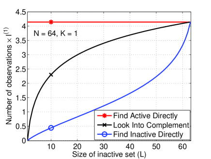
Figure 2: Sufficiency bounds on the number of observations required to find $L$ inactive variables for $K=1$ case. The comparison is presented with respect to the value of $MI^{(1)}$, as the application-dependent mutual information term $I^{(1)}$ is common to all the bounds. The approach of finding the $L$ inactive variables directly, especially for small values of $L$, requires significantly fewer number of observations compared to the approach of finding the inactive variables indirectly, after first identifying the active variables. The plot corresponding to the curve labeled Find Active Directly refers to the number of observations that are sufficient for finding the $K$ active variables[21].

IV Necessary Number of Observations

In this section, we derive lower bounds on the number of observations required to find a set of $L$ inactive variables, in the sense that if the number of observations is lower than the bound, the probability of error will be bounded strictly away from zero, regardless of the decoding algorithm used. Here, we need to lower bound the probability of error in choosing a set of $L$ inactive variables. To this end, we employ an adaptation of Fano’s inequality [34, 35].

Let $\mathcal{I}^{d}\triangleq\left\{\omega_{1},\omega_{2},\ldots,\omega_{N\choose K}\right\}$ be the collection of all $K$ sized subsets of $[N]$ such that $|S_{\omega_{i}}|=K$ for $i=1,2,\ldots,{N\choose K}$. For each $\omega\in\mathcal{I}^{d}$ let us associate a collection of sets, $\mathcal{I}^{h}_{\omega}\triangleq\left\{\alpha_{1},\alpha_{2},\ldots,\alpha_{N-K\choose L}\right\}$, such that $|S_{\alpha_{i}}|=L$ and $S_{\alpha_{i}}\cap S_{\omega}=\{0\}$, $i=1,2,\ldots,{N-K\choose L}$. That is, $\mathcal{I}^{h}_{\omega}$ is the collection of all $L$-sized subsets of all-inactive variables when $S_{\omega}$ represents the active set. Also, let $\mathcal{I}^{H}$ denote the set of all $L$-sized subsets of $[N]$. Note that $|\mathcal{I}^{H}|={N\choose L}$. Given the observation vector, $\underline{\mathbf{y}}\in\mathcal{Y}^{M}$, let $\phi:\mathcal{Y}^{M}\rightarrow\mathcal{I}^{H}$ denote a decoding function, such that $\hat{\alpha}=\phi(\underline{\mathbf{y}})$ is the decoded set of $L$ inactive variables. Given an active set $\omega$ and an observation vector $\underline{\mathbf{y}}$, an error occurs if $\hat{\alpha}\notin\mathcal{I}^{h}_{\omega}$. Define,

$$P_{e}=P(\hat{\alpha}\notin\mathcal{I}^{h}_{\omega}).$$ (10)

Define a binary error RV, $E$, as $E\triangleq\mathbb{I}_{\left\{\hat{\alpha}\notin\mathcal{I}^{h}_{\omega}\right\}}$. Note that $P_{e}=\text{Pr}(E=1)$. We state a necessary condition on the number of observations in the following theorem.

Theorem 3.

Let $N$, $M$, $L$ and $K$ be as defined before. Let $I^{(j)}$ and $P_{e}$ be as defined in (4) and (10), respectively. A necessary condition on the number of observations $M$ required to find $L$ inactive variables with asymptotically vanishing probability of error, i.e., $\lim_{N\rightarrow\infty}P_{e}=0$, is given by

$$M \geq\max_{1\leq j\leq K}\frac{\Gamma_{l}(L,N,K,j)}{I^{(j)}}(1-\eta),~{}~{}\mbox{where}~{}~{}~{}\Gamma_{l}(L,N,K,j)\triangleq\log\left[\frac{{N-K+j\choose j}}{{N-K+j-L\choose j}}\right],$$ (11)

for some $\eta>0$.

Proof: See Sec. VI-C.

That is, any sequence of random codebooks, that achieves $\lim_{N\rightarrow\infty}P_{e}=0$, must satisfy the above bound on the length of the codewords. Given a specific application, we can bound $I^{(j)}$ for each $j=1,2,\ldots,K$, and obtain a characterization on the necessary number of observations, as we show in the next section.

V Finding Non-Defective Items Via Group Testing

In this section, we apply the above mutual information based results to the specific case of non-adaptive group testing, and characterize the number of tests to identify a subset of non-defective items in a large population. We consider a random pooling based, noisy non-adaptive group testing framework[21, 4], as described in detail in Section II. Our goal here is to find upper and lower bounds on the number of tests required to identify an $L$ sized subset belonging to $[N]\backslash\mathcal{G}$ using the observations $\underline{y}$, with vanishing probability of error as $N\rightarrow\infty$. We focus on the regime where $K,L,N\rightarrow\infty$ with $\frac{L}{N-K}\rightarrow\alpha_{0}$, $\frac{K}{N-K}\rightarrow\beta_{0}$ for some fixed $\alpha_{0},\beta_{0}\in(0,1)$.

To compute the lower bounds on the number of tests, using the results of Theorem 3, we need to upper bound the mutual information term, $I^{(j)}$, for the group testing signal model given in (2). Using the bounds on $I^{(j)}$[41], with $p=\frac{1}{K}$ and $u\leq 0.5$, we summarize the order-accurate lower bounds on the number of tests to find a set of $L$ non-defective items in Table I. A brief sketch of the derivation of these results is provided in Appendix -B.

To compute the upper bounds on the number of tests, we need to lower bound $E_{0}(\rho,1,n)$ for some $\rho\in[0,1]$ and show that the negative exponent in the probability of error term in (9) can be made strictly greater than $0$ by choosing $M$ sufficiently large. We first present the lower bounds on $E_{0}(\rho,1,n)$ in the following lemma.

Lemma 1.

Let $N$, $M$, $L$ and $K$ be as defined above. Let $L_{0}=(N-L-2K+1)$. Let $E_{0}(\rho,j,n)$ be as defined in (3) and define $\rho_{0}\triangleq\frac{K-1}{L_{0}}$. For the non-adaptive group testing model with $p=\frac{1}{K}$ and for all values of $L\leq(N-3K+1)$, we have

1. For the noiseless case ($u=0,q=0$):

   $$E_{0}(\rho_{0},1,L_{0})\geq\frac{(1-e^{-1})-(\frac{1}{K})^{K}}{e}$$ (12)

2. For the additive noise only case ($u=0,q>0$):

   $$E_{0}(\rho_{0},1,L_{0})\geq\frac{e^{-2}}{4}(1-q)$$ (13)

3. For the dilution noise only case ($u>0,q=0$):

   $$E_{0}(\rho_{0},1,L_{0})\geq\frac{e^{-2}}{4}(1-u^{\frac{1}{K}})$$ (14)

The proof of the above lemma is presented in Appendix -A. For notational convenience, we let $E_{0}^{(lb)}$ denote a common lower bound on $E_{0}(\rho_{0},1,L_{0})$, as derived above. The following lemma presents an upper bound on the number of tests required to identify $L$ non-defective items in a non-adaptive group testing setup.

Theorem 4.

Let $P_{e}$ be the average probability of error in finding $L$ inactive variables under the decoding scheme described in Section III-B2, which is upper bounded by (9). Let $L_{0}\triangleq(N-L-2K+1)$ and let $\theta_{0}\triangleq\frac{L+K-1}{N-K}$. Then, for any $\epsilon_{0}>0$ and all values of $L\leq(N-3K+1)$, if $M$ is chosen as

$$M>(1+\epsilon_{0})\frac{K-1}{E_{0}^{(lb)}}\left[\frac{H_{b}(\theta_{0})}{1-\theta_{0}}+\log\left(2+\frac{L}{K-1}\right)+1+\frac{\log K}{K-1}\right],$$ (15)

then $P_{e}\leq\exp\left(-\epsilon_{0}(K-1)\log\frac{N-K}{L_{0}}\right)$.

An outline of the proof is presented in Section VI-D. In the regime where $L,K\rightarrow\infty$ as $N\rightarrow\infty$, it follows from the above lemma that $\lim_{N\rightarrow\infty}P_{e}=0$.

Finally, we present an upper bound on the number of tests obtained for the indirect decoding scheme presented in Section III-A for the noiseless case. Using [21, Lemma VII.$1$ and VII.$3$] to lower bound $E_{0}(\rho,j,1)$ for the noiseless case, and noting that, from the union bound, we have $C_{0}(j)\leq\frac{j{N-K-1\choose L-1}}{{N-K\choose L}}=j\frac{L}{N-K}$, the following corollary builds on the results presented in Corollary 1.

Corollary 2.

Let $P_{e}$ be the average probability of error in finding $L$ inactive variables under the decoding scheme described in Section III-A, which is upper bounded by (5). For any $\epsilon_{0}>0$, there exists absolute constant $c_{0}>2$, independent of $N$, $K$ and $L$, such that if $M$ is chosen as

$$M>(1+\epsilon_{0})c_{0}K\log L\log^{2}K,$$ (16)

then $P_{e}\leq\exp\left(-\epsilon_{0}(K\log L)\right)$.

We now make following observations about the results presented in this section. We consider the regime where for some fixed $\alpha_{0},\beta_{0}\in(0,1)$, $\frac{L}{N-K}\rightarrow\alpha_{0}$, $\frac{K}{N-K}\rightarrow\beta_{0}$ as $N\rightarrow\infty$. Further, as we are typically interested in $L\geq K$ and, also since our results apply for $L\leq N-3K+1$, we only consider $\alpha_{0}$, $\beta_{0}$ such that $\beta_{0}\leq\alpha_{0}$ and $\alpha_{0}+2\beta_{0}\leq 1$. For the indirect decoding scheme presented in Section III-B, we summarize the upper bounds on the number of tests to find a set of $L$ non-defective items in Table II.

1. We first consider the noiseless case.

   1. For the direct decoding scheme, $O(K)$ number of tests are sufficient. In comparison, using results from Corollary 2, $O(K\log L\log^{2}K)$ tests are sufficient for the indirect decoding scheme. Also, from [21, Theorem V.2], $O(K\log N\log^{2}K)$ tests are sufficient for finding all the defective items. Thus, in this case, the direct decoding scheme for finding non-defective items performs better compared to the indirect decoding schemes by a poly-log factor of the number of defective items, $K$. Further, from Table I, we observe that the upper bound on the number of tests for the direct decoding scheme is within a $c\log K$ factor of the lower bound, where $c$ is a constant independent of $N$, $L$ and $K$.

   2. The size of non-defective set, $L$, impacts the upper bound on the number of tests only through $\alpha_{0}$, i.e., the fraction of non-defective items that need to be found. From Table II, $\Phi(\alpha_{0},\beta_{0})$ is an increasing function of $\alpha_{0}$. That is, a higher $\alpha_{0}$ results in a higher rate at which the upper bound on the number of tests increases with $K$.

2. Performance under noisy observations:

   1. For the additive noise, $O(\frac{K}{1-q})$ number of tests are sufficient for the direct decoding scheme The indirect scheme (as well as finding the defective items) also show similar $\frac{1}{1-q}$ factor increase in the number of tests under additive noise scenario (see, e.g., [21, Theorem VI.2]). Further, from Table I, we observe that for fixed $\alpha_{0},\beta_{0}$ and $q$, the upper bound on the number of tests for the direct decoding scheme is within a constant factor of the lower bound.

   2. For dilution noise, $O\left(\frac{K}{1-u^{\frac{1}{K}}}\right)$ are sufficient for the direct decoding scheme. Another characterization for the sufficient number of tests for the direct decoding scheme, based on the remark at the end of Appendix -A, is $O\left(\frac{K^{2}}{1-u^{\frac{1}{2}}}\right)$ number of tests. The direct decoding scheme shows high sensitivity to the dilution noise. This behavior is in sharp contrast to the indirect scheme, where the dilution noise parameter $u$ leads to an increase in the number of tests only by a factor of $\frac{c}{1-u}$ (see, e.g., [21, Theorem VI.5]). From Table I, the lower bounds also show an increase in the number of tests by a factor $\frac{1}{1-u}$ for the dilution noise scenario. The conservativeness of the upper bound for the direct decoding scheme in the presence of dilution noise appears to be due to the following factors: (a) The lower bound on $E_{0}$ is $\Omega(\frac{1}{K})$, which underscores the general fact that the group testing system is more sensitive to the diluton noise, and (b) The term $\log{N-1-L_{0}\choose K-1}$ in (9), which might be due to the particular decoding scheme employed or the specific technique employed in bounding the error exponent.

TABLE I: Finding a subset of $L$ non-defective items: Results for necessary number of group tests which hold asymptotically as $(N,K,L)\rightarrow\infty$, $\frac{L}{N-K}\rightarrow\alpha_{0}$ with $0<\alpha_{0}<1$. The constants $C_{n},C_{n}^{\prime},C_{n}^{\prime\prime}>0$ are independent of $N,L,K,u$ and $q$.

No Noise	$\dfrac{C_{n}K}{\log K}\log\dfrac{1}{[1-\alpha_{0}+o(1)]}$
Additive Noise	$\dfrac{C_{n}^{\prime}K}{\log\frac{1}{q}}\log\dfrac{1}{[1-\alpha_{0}+o(1)]}$
Dilution Noise	$\dfrac{C_{n}^{\prime\prime}K}{(1-u)\log K}\log\dfrac{1}{[1-\alpha_{0}+o(1)]}$

TABLE II: Finding a subset of $L$ non-defective items: Results for sufficient number of group tests which hold asymptotically as $(N,K,L)\rightarrow\infty$, $\frac{L}{N-K}\rightarrow\alpha_{0}$ and $\frac{K}{N-K}\rightarrow\beta_{0}$ with $0<\beta_{0}\leq\alpha_{0}<1$ such that $\alpha_{0}+2\beta_{0}<1$. Define $\Phi(\alpha_{0},\beta_{0})\triangleq\left(\frac{H_{b}(\gamma_{0})}{1-\gamma_{0}}+\log\frac{\alpha_{0}}{\beta_{0}}\right)$, where $\gamma_{0}=\alpha_{0}+\beta_{0}$. The constants $C_{s},C_{s}^{\prime},C_{s}^{\prime\prime}>0$ are independent of $N,L,K,u$ and $q$.

No Noise	$\dfrac{C_{s}K}{(1-o(1))}\left[\Phi(\alpha_{0},\beta_{0})+o(1)\right]$
Additive Noise	$\dfrac{C_{s}^{\prime}K}{(1-q)}\left[\Phi(\alpha_{0},\beta_{0})+o(1)\right]$
Dilution Noise	$\dfrac{C_{s}^{\prime\prime}K}{(1-u^{\frac{1}{K}})}\left[\Phi(\alpha_{0},\beta_{0})+o(1)\right]$

VI Proofs of the Main Results

We now present the proofs of Theorems 1, 2 and 3, which constitute the main results in this paper.

VI-A Proof of Theorem 1: Sufficient Number of Observations, $K=1$ Case

At the heart of the proof of this theorem is the derivation of an upper bound on the average probability of error in finding $L$ inactive variables using the decoding scheme described in Section III-B1. In turn, the upper bound is obtained by characterizing the error exponents on the average probability of error [34]. Without loss of generality, due to the symmetry in the model, we can assume that the RV $X_{1}$ is active. Given that $X_{1}$ is the active variable, the decoding algorithm will make an error if $P(\underline{\mathbf{y}}|\mathbf{X}_{1})$ falls within the last $L$ entries of the sorted array generated as described in the decoding scheme. Let $\underline{\mathbf{y}}$ be the observed output, and let $\mathcal{E}$ denote the event that an error has occurred, when item $X_{1}$ is the active variable and $\mathbf{X}_{1}$ is the first column of $\mathbf{X}$. Further, let $\text{Pr}(\mathcal{E})$ be a shorthand for $\text{Pr}\{\text{error}|X_{1}\text{ is active},\mathbf{X}_{1},\underline{\mathbf{y}}\}$. The overall average probability of error, $P_{e}$, can be expressed as

$$P_{e} =\sum_{\underline{\mathbf{y}},\mathbf{X}_{1}}P(\underline{\mathbf{y}}|\mathbf{X}_{1})Q(\mathbf{X}_{1})\text{Pr}(\mathcal{E}).$$ (17)

Let $S_{z}\subset[N]\backslash 1$ be a set of $N-L$ items, i.e., $|S_{z}|=N-L$. Let $\mathbf{\mathcal{S}_{z}}$ denote the set of all possible $S_{z}$. Further, let $\mathcal{A}_{S_{z}}\subset\{\mathbf{X}_{S_{z}}\}$ be such that, $\mathcal{A}_{S_{z}}=\{\{\mathbf{X}_{S_{z}}\}:P(\underline{\mathbf{y}}|\mathbf{X}_{j})~{}\geq~{}P(\underline{\mathbf{y}}|\mathbf{X}_{1})~{}\forall~{}j\in S_{z}\}$. That is, $\mathcal{A}_{S_{z}}$ represents all those realizations of the random variable $\mathbf{X}_{S_{z}}$ which satisfy the above condition, which states that each variable in $S_{z}$ is more likely than the active variable, $X_{1}$. It is easy to see that $\mathcal{E}\subset\mathcal{A}\triangleq\bigcup_{{S_{z}}\in\mathcal{S}_{z}}\mathcal{A}_{S_{z}}$, i.e., an error event implies that there exists at least one set of $N-L$ variables, $S_{z}$, such that $P(\underline{\mathbf{y}}|\mathbf{X}_{j})~{}\geq~{}P(\underline{\mathbf{y}}|\mathbf{X}_{1})~{}\forall~{}j\in S_{z}$. Thus, $\text{Pr}(\mathcal{E})\leq\text{Pr}(\mathcal{A})$. Let $s$ be an optimization variable such that $0\leq s\leq 1$. The following set of inequalities upper bound $\text{Pr}(\mathcal{E})$:

$$\text{Pr}(\mathcal{E}) \leq\sum_{S_{z}\in\mathbf{\mathcal{S}_{z}}}~{}\sum_{\mathbf{X}_{S_{z}}\in\mathcal{A}_{S_{z}}}Q(\mathbf{X}_{S_{z}})$$

$$\mathrel{\overset{\textrm{(a)}}{\vphantom{\leq}{\leq}}}\sum_{S_{z}\in\mathbf{\mathcal{S}_{z}}}~{}\sum_{\mathbf{X}_{S_{z}}\in\mathcal{A}_{S_{z}}}Q(\mathbf{X}_{S_{z}})\prod_{j\in S_{z}}\left[\frac{P(\underline{\mathbf{y}}|\mathbf{X}_{j})}{P(\underline{\mathbf{y}}|\mathbf{X}_{1})}\right]^{s}$$

$$\mathrel{\overset{\textrm{(b)}}{\vphantom{\leq}{\leq}}}\sum_{S_{z}\in\mathbf{\mathcal{S}_{z}}}~{}\sum_{\mathbf{X}_{S_{z}}}~{}\prod_{j\in S_{z}}Q(\mathbf{X}_{j})\left[\frac{P(\underline{\mathbf{y}}|\mathbf{X}_{j})}{P(\underline{\mathbf{y}}|\mathbf{X}_{1})}\right]^{s}$$

$$\mathrel{\overset{\textrm{(c)}}{\vphantom{\leq}{=}}}\sum_{S_{z}\in\mathbf{\mathcal{S}_{z}}}~{}\prod_{j\in S_{z}}~{}\sum_{\mathbf{X}_{j}}Q(\mathbf{X}_{j})\left[\frac{P(\underline{\mathbf{y}}|\mathbf{X}_{j})}{P(\underline{\mathbf{y}}|\mathbf{X}_{1})}\right]^{s}$$

$$\mathrel{\overset{\textrm{(d)}}{\vphantom{\leq}{=}}}{N-1\choose L-1}\left\{\sum_{\mathbf{X}_{j}}Q(\mathbf{X}_{j})\left[\frac{P(\underline{\mathbf{y}}|\mathbf{X}_{j})}{P(\underline{\mathbf{y}}|\mathbf{X}_{1})}\right]^{s}\right\}^{N-L}.$$ (18)

In the above, (a) follows since we are multiplying with terms that are all greater than $1$ and $(b)$ follows since we are adding extra nonnegative terms by summing over all $\mathbf{X}_{S_{z}}$. $(c)$ follows by using the independence of the codewords, i.e., $Q(\mathbf{X}_{S_{z}})=\prod_{j\in S_{z}}Q(\mathbf{X}_{j})$, and simplifying further. $(d)$ follows since the value of the expression inside the product term does not depend upon any particular $j$.

Let $0\leq\rho\leq 1$. If the R.H.S. in (18) is less than $1$, then raising it to the power $\rho$ makes it bigger, and if it is greater than $1$, it remains greater than $1$ after raising it to the power $\rho$. Thus, we get the following upper bound on $\text{Pr}(\mathcal{E})$:

$$\text{Pr}(\mathcal{E}) \leq{N-1\choose L-1}^{\rho}\left\{\sum_{\mathbf{X}_{j}}Q(\mathbf{X}_{j})\left[\frac{P(\underline{\mathbf{y}}|\mathbf{X}_{j})}{P(\underline{\mathbf{y}}|\mathbf{X}_{1})}\right]^{s}\right\}^{\rho(N-L)}.$$ (19)

Substituting this into (17) and simplifying, we get

$$P_{e}\leq{N-1\choose L-1}^{\rho}\sum_{\underline{\mathbf{y}}}\sum_{\mathbf{X}_{1}}Q(\mathbf{X}_{1})P(\underline{\mathbf{y}}|\mathbf{X}_{1})^{1-\rho(N-L)s}\left\{\sum_{\mathbf{X}_{j}}Q(\mathbf{X}_{j})P(\underline{\mathbf{y}}|\mathbf{X}_{j})^{s}\right\}^{\rho(N-L)}.$$ (20)

Putting $s=1/(1+\rho(N-L))$, we get

$$P_{e}\leq{N-1\choose L-1}^{\rho}\sum_{\underline{\mathbf{y}}}\left\{\sum_{\mathbf{X}_{j}}Q(\mathbf{X}_{j})P(\underline{\mathbf{y}}|\mathbf{X}_{j})^{\frac{1}{1+\rho(N-L)}}\right\}^{1+\rho(N-L)}.$$ (21)

Finally, using the independence across observations and using the definition of $E_{0}(\rho,j,n)$ from (3) with $j=1$ and $n=N-L$, we get

$$P_{e} \leq{N-1\choose L-1}^{\rho}\left[\sum_{Y\in\mathcal{Y}}\left\{\sum_{X_{j}\in\mathcal{X}}Q(X_{j})P(Y|X_{j})^{\frac{1}{1+\rho(N-L)}}\right\}^{1+\rho(N-L)}\right]^{M}$$

$$=\exp^{\left[-MF(\rho)\right]},~{}\mbox{where}~{}F(\rho)=E_{0}(\rho,1,N-L)-\frac{\rho\log{N-1\choose L-1}}{M}.$$ (22)

Hence (6) follows.

For the following discussion, we treat $F$ and $E_{0}$ as functions of $\rho$ only and all the derivatives are with respect to $\rho$. Note that $F^{{}^{\prime}}(\rho)=E_{0}^{{}^{\prime}}(\rho)-\frac{\log{N-1\choose L-1}}{M}$. It is easy to see that $E_{0}(0)=0$ and hence $F(0)=0$. With some calculation, we get,

$$\left.E_{0}^{{}^{\prime}}(\rho)\right|_{\rho=0}=(N-L)\sum_{Y,X}P(Y,X)\log\frac{P(Y|X)}{P(Y)}=(N-L)I^{(1)}.$$ (23)

Using the Taylor series expansion of $E_{0}(\rho)$, and following similar analysis as in [21, Section III.D], it is easy to show that there exists a $\rho\in(0,1]$, sufficiently small, such that if $M$ is chosen as in (7), then $MF(\rho)>\epsilon_{1}(N-L)\log{N-1\choose L-1}$ for some $\epsilon_{1}>0$, independent of $N$ and $L$. This completes the proof.

Remark: For the decoding scheme described in III-A, for the $K=1$ case, using similar arguments as the above, if $M>(1+\epsilon_{0})\frac{\log(L-1)}{I^{(1)}}$ for any $\epsilon_{0}>0$, then there exists $\epsilon_{1}>0$, and independent of $N$ and $L$, such that $P_{e}\leq\exp(-\epsilon_{1}\log L)$, i.e., $P_{e}\rightarrow 0$, as $L\rightarrow\infty$.

VI-B Proof of Theorem 2: Sufficient Number of Observations, $K>1$ Case

The decoding algorithm outputs a set, $S_{H}$, of at least $L$ inactive variables. A decoding error happens if the set $S_{H}$ contains one or more variables from the active set. We now upper bound the average probability of error of the proposed decoding algorithm. The probability is averaged over all possible instantiations of $\{\mathbf{X},\underline{\mathbf{y}}\}$ as well as over all possible active sets. By symmetry of the codebook ($\mathbf{X}$) construction, the average probability of error is the same for all the active sets. Hence, we fix the active set and then compute average probability of error with this set. Let $S_{1}\subset[N]$ be the active set such that $|S_{1}|=K$. We also define the following notation: For any set $S_{\omega}\subset[N]$ such that $|S_{\omega}|=K$ and for any item $j\in S_{\omega}$, let $S_{\omega j^{c}}\triangleq S_{\omega}\backslash j$. Note that $|S_{\omega j^{c}}|=K-1$.

For any $d\in S_{1}$, define $\mathcal{E}_{d}$ to be the error event such that $d$ belongs to $S_{H}$. The overall average probability of error, $P_{e}$, in finding $L$ inactive variables can thus be upper bounded as

$$P_{e}\leq\sum_{d\in S_{1}}\text{Pr}({\mathcal{E}_{d}}).$$ (24)

Further,

$$\text{Pr}({\mathcal{E}_{d}})=\sum_{\underline{\mathbf{y}}}\sum_{\mathbf{X}_{S_{1}}}P(\underline{\mathbf{y}}|\mathbf{X}_{S_{1}})Q(\mathbf{X}_{S_{1}})\left[\text{Pr}\{\mathcal{E}_{d}|S_{1}~{}\mbox{is the active set},\underline{\mathbf{y}},\mathbf{X}_{S_{1}}\}\right].$$ (25)

We now upper bound $\text{Pr}\{\mathcal{E}_{d}|S_{1}~{}\mbox{is the active set},\underline{\mathbf{y}},\mathbf{X}_{S_{1}}\}$. Let $S_{z}\subset[N]\backslash S_{1}$ be such that $|S_{z}|=L_{0}$. Let $S_{\omega}\subset[N]$ be a $K$ sized index set such that $S_{\omega}=\{d\cup S_{\omega d^{c}}\}$, where $S_{\omega d^{c}}\subset[N]\backslash\{d\}\backslash S_{z}$ and $d\in S_{1}$. Further, let $\mathbf{\mathcal{S}_{z}}$ and $\mathbf{\mathcal{S}_{\omega d^{c}}}$ be the collection of all possible sets $S_{z}$ and $S_{\omega d^{c}}$, respectively. It is easy to see that $|\mathbf{\mathcal{S}_{z}}|={N-K\choose L_{0}}$ and $|\mathbf{\mathcal{S}_{\omega d^{c}}}|={N-1-L_{0}\choose K-1}$. With $S_{1}$ as the active set, $d\in S_{1}$, the observed output $\underline{\mathbf{y}}$ and the codebook entries corresponding to set $S_{1}$ as $\mathbf{X}_{S_{1}}$, define $\mathcal{A}_{d}({S_{z},S_{\omega d^{c}}})\subset\{\mathbf{X}_{S_{z}\cup S_{\omega d^{c}}}\}$ and $\mathcal{A}_{d}$ as follows:

$$\mathcal{A}_{d}({S_{z},S_{\omega d^{c}}}) =\{\{\mathbf{X}_{S_{z}},\mathbf{X}_{S_{\omega d^{c}}}\}:~{}P(\underline{\mathbf{y}}|\mathbf{X}_{\alpha},\mathbf{X}_{S_{\omega d^{c}}})\geq P(\underline{\mathbf{y}}|\mathbf{X}_{d},\mathbf{X}_{S_{\omega d^{c}}})~{}\forall~{}{\alpha}\in S_{z}\},$$ (26)

$$\mathcal{A}_{d} =\bigcup_{S_{z}\in\mathcal{S}_{z}}\bigcup_{S_{\omega d^{c}}\in\mathcal{S}_{\omega d^{c}}}\mathcal{A}_{d}({S_{z},S_{\omega d^{c}}}).$$ (27)

That is, $\mathcal{A}_{d}(S_{z},S_{\omega d^{c}})$ represents a set of the those realizations of the random variables $\mathbf{X}_{S_{z}}$ and $\mathbf{X}_{S_{\omega d^{c}}}$ which satisfy the condition in (26).

Proposition 1.

$\text{Pr}\{\mathcal{E}_{d}|S_{1}~{}\mbox{is the active set},\underline{\mathbf{y}},\mathbf{X}_{S_{1}}\}\leq\text{Pr}(\mathcal{A}_{d})$

Proof.

We will show that given the active set $S_{1}$, $d\in S_{1}$, $\underline{\mathbf{y}}$ and $\mathbf{X}_{S_{1}}$, the event $\{d\in S_{H}\}$, i.e., the decoded set of inactive variables contains $d$, implies the event $\mathcal{A}_{d}$. We first note that, since $|S_{H}|\leq L+K-1$, there exists a set of $L_{0}=N-K-(L+K-1)$ inactive variables that do not belong to $S_{H}$. Let $S_{z}\subset[N]\backslash S_{1}$ be such a set of inactive variables such that $|S_{z}|=L_{0}$ and $S_{z}\cap S_{H}=\{\emptyset\}$.

Further, since $d\in S_{H}$, this implies that there exits an $\omega\in\Omega_{\text{last}}$ such that $d$ belongs to $S_{\omega}$, where $\Omega_{\text{last}}$ is as defined in the decoding scheme for $K>1$ (see Section III-B2). With the notation described above, we can represent such $S_{\omega}$ as $\{d\cup S_{\omega d^{c}}\}$, where $S_{\omega d^{c}}\subset[N]\backslash\{d\}\backslash S_{z}$ such that $|S_{\omega d^{c}}|=K-1$. For any $\alpha\in S_{z}$, if we replace $d\in S_{\omega}$ with $\alpha$ and evaluate $P(\underline{\mathbf{y}}|\mathbf{X}_{\alpha},\mathbf{X}_{S_{\omega d^{c}}})$, it cannot be smaller than $P(\underline{\mathbf{y}}|\mathbf{X}_{d},\mathbf{X}_{S_{\omega d^{c}}})$ or else the decoding algorithm would have chosen $\alpha$ as belonging to $S_{H}$. This implies that, there exists a realization of $\mathbf{X}_{S_{z}}$ and $\mathbf{X}_{S_{\omega d^{c}}}$ such that $P(\underline{\mathbf{y}}|\mathbf{X}_{\alpha},\mathbf{X}_{S_{\omega d^{c}}})\geq P(\underline{\mathbf{y}}|\mathbf{X}_{d},\mathbf{X}_{S_{\omega d^{c}}})~{}\forall~{}{\alpha}\in S_{z}$, i.e., ${\mathcal{A}_{d}}$ occurs. ∎

We now upper bound $\text{Pr}(\mathcal{A}_{d})$ as follows:

$$\text{Pr}(\mathcal{A}_{d})\leq\sum_{S_{z}\in\mathbf{\mathcal{S}_{z}}}~{}\sum_{S_{\omega d^{c}}\in\mathbf{\mathcal{S}_{\omega d^{c}}}}~{}q_{d},$$ (28)

where $q_{d}\triangleq\text{Pr}\{\mathcal{A}_{d}(S_{z},S_{\omega d^{c}})|S_{1}~{}\mbox{is active set},\underline{\mathbf{y}},\mathbf{X}_{S_{1}}\}$. Here, the randomness comes from the set of variables in $S_{z}$ and $S_{\omega d^{c}}$, i.e., $\mathbf{X}_{S_{z}}$ and $\mathbf{X}_{S_{\omega d^{c}}}$. Let $s$ be such that $0\leq s\leq 1$. We have

$$q_{d} =\sum_{\mathbf{X}_{S_{z}},\mathbf{X}_{S_{\omega d^{c}}}\in\mathcal{A}_{d}({S_{z},S_{\omega d^{c}}})}Q(\mathbf{X}_{S_{z}},\mathbf{X}_{S_{\omega d^{c}}})$$

$$\mathrel{\overset{\textrm{(a)}}{\vphantom{\leq}{\leq}}}\sum_{\mathbf{X}_{S_{\omega d^{c}}},\mathbf{X}_{S_{z}}\in\mathcal{A}_{d}({S_{z},S_{\omega d^{c}}})}Q(\mathbf{X}_{S_{z}},\mathbf{X}_{S_{\omega d^{c}}})\prod_{S_{\alpha}\in S_{z}}\left[\frac{P(\underline{\mathbf{y}}|\mathbf{X}_{\alpha},\mathbf{X}_{S_{\omega d^{c}}})}{P(\underline{\mathbf{y}}|\mathbf{X}_{d},\mathbf{X}_{S_{\omega d^{c}}})}\right]^{s}$$

$$\mathrel{\overset{\textrm{(b)}}{\vphantom{\leq}{\leq}}}\sum_{\mathbf{X}_{S_{\omega d^{c}}}}~{}Q(\mathbf{X}_{S_{\omega d^{c}}})~{}\sum_{\mathbf{X}_{S_{z}}}~{}Q(\mathbf{X}_{S_{z}})\prod_{S_{\alpha}\in S_{z}}\left[\frac{P(\underline{\mathbf{y}}|\mathbf{X}_{\alpha},\mathbf{X}_{S_{\omega d^{c}}})}{P(\underline{\mathbf{y}}|\mathbf{X}_{d},\mathbf{X}_{S_{\omega d^{c}}})}\right]^{s}$$

$$\mathrel{\overset{\textrm{(c)}}{\vphantom{\leq}{=}}}\sum_{\mathbf{X}_{S_{\omega d^{c}}}}Q(\mathbf{X}_{S_{\omega d^{c}}})\prod_{l=1}^{L_{0}}\sum_{\mathbf{X}_{S_{\alpha}}}Q(\mathbf{X}_{S_{\alpha}})\left[\frac{P(\underline{\mathbf{y}}|\mathbf{X}_{\alpha},\mathbf{X}_{S_{\omega d^{c}}})}{P(\underline{\mathbf{y}}|\mathbf{X}_{d},\mathbf{X}_{S_{\omega d^{c}}})}\right]^{s}$$

$$\mathrel{\overset{\textrm{(d)}}{\vphantom{\leq}{=}}}\sum_{\mathbf{X}_{S_{\omega d^{c}}}}Q(\mathbf{X}_{S_{\omega d^{c}}})\left\{\sum_{\mathbf{X}_{S_{\alpha}}}Q(\mathbf{X}_{S_{\alpha}})\left[\frac{P(\underline{\mathbf{y}}|\mathbf{X}_{\alpha},\mathbf{X}_{S_{\omega d^{c}}})}{P(\underline{\mathbf{y}}|\mathbf{X}_{d},\mathbf{X}_{S_{\omega d^{c}}})}\right]^{s}\right\}^{L_{0}}$$

$$=\sum_{\mathbf{X}_{S_{\omega d^{c}}}}Q(\mathbf{X}_{S_{\omega d^{c}}})\underbrace{\left\{\sum_{\mathbf{X}_{S_{\alpha}}}Q(\mathbf{X}_{S_{\alpha}})\left[\frac{P(\underline{\mathbf{y}},\mathbf{X}_{S_{\omega d^{c}}}|\mathbf{X}_{\alpha})}{P(\underline{\mathbf{y}},\mathbf{X}_{S_{\omega d^{c}}}|\mathbf{X}_{d})}\right]^{s}\right\}^{L_{0}}}_{\triangleq\mathcal{P}_{0}(\underline{\mathbf{y}},\mathbf{X}_{d},\mathbf{X}_{S_{\omega d^{c}}})}.$$ (29)

In the above, (a)-(d) follow using the same reasoning as in (18) in the proof of Theorem 1 (Section VI-A). We note that, due to symmetry in the construction of codebook, $\mathcal{P}_{0}(\underline{\mathbf{y}},\mathbf{X}_{d},\mathbf{X}_{S_{\omega d^{c}}})$ does not depend upon the index set $S_{z}$ or $\mathbf{X}_{S_{z}}$. In fact, it depends only upon the given realizations of $\mathbf{X}_{S_{\omega d^{c}}}$, $\mathbf{X}_{d}$ and not on the particular index sets $S_{\omega d^{c}}$ and $d$, respectively. Thus, from (28), and for some $0\leq\rho\leq 1$, we get

$$\text{Pr}(\mathcal{A}_{d}) \leq\sum_{S_{\omega d^{c}}\in\mathbf{\mathcal{S}_{\omega d^{c}}}}\sum_{\mathbf{X}_{S_{\omega d^{c}}}}Q(\mathbf{X}_{S_{\omega d^{c}}})\left[\sum_{S_{z}\in\mathcal{S}_{z}}\mathcal{P}_{0}(\underline{\mathbf{y}},\mathbf{X}_{d},\mathbf{X}_{S_{\omega d^{c}}})\right]$$ (30)

$$\leq\sum_{S_{\omega d^{c}}\in\mathbf{\mathcal{S}_{\omega d^{c}}}}\sum_{\mathbf{X}_{S_{\omega d^{c}}}}Q(\mathbf{X}_{S_{\omega d^{c}}})\left[\sum_{S_{z}\in\mathcal{S}_{z}}\mathcal{P}_{0}(\underline{\mathbf{y}},\mathbf{X}_{d},\mathbf{X}_{S_{\omega d^{c}}})\right]^{\rho}$$ (31)

$$\leq{N-1-L_{0}\choose K-1}\sum_{\mathbf{X}_{S_{\omega d^{c}}}}Q(\mathbf{X}_{S_{\omega d^{c}}})\left[{N-K\choose L_{0}}\mathcal{P}_{0}(\underline{\mathbf{y}},\mathbf{X}_{d},\mathbf{X}_{S_{\omega d^{c}}})\right]^{\rho}.$$ (32)

The second inequality above follows since the expression inside the square brackets represents the probability of a union of events and thus, as in $K=1$ case, by raising it to a power $0<\rho\leq 1$, we still get an upper bound [34, Section 5.6]. Let $C_{2}\triangleq{N-K\choose L_{0}}^{\rho}{N-1-L_{0}\choose K-1}$. Using proposition 1, we substitute the above expression into (24) to get:

$$\text{Pr}({\mathcal{E}_{d}}) \leq~{}C_{2}\sum_{\underline{\mathbf{y}}}\sum_{\mathbf{X}_{S_{1}}}Q(\mathbf{X}_{S_{1}})P(\underline{\mathbf{y}}|\mathbf{X}_{S_{1}})\sum_{\mathbf{X}_{S_{\omega d^{c}}}}Q(\mathbf{X}_{S_{\omega d^{c}}})\left[\mathcal{P}_{0}(\underline{\mathbf{y}},\mathbf{X}_{d},\mathbf{X}_{S_{\omega d^{c}}})\right]^{\rho}$$

$$\mathrel{\overset{\textrm{(a)}}{\vphantom{\leq}{\leq}}}~{}C_{2}\sum_{\underline{\mathbf{y}}}\sum_{\mathbf{X}_{S_{1}}}\sum_{\mathbf{X}_{S_{\omega d^{c}}}}Q(\mathbf{X}_{S_{1}})P(\underline{\mathbf{y}},\mathbf{X}_{S_{\omega d^{c}}}|\mathbf{X}_{S_{1}})\left[\mathcal{P}_{0}(\underline{\mathbf{y}},\mathbf{X}_{d},\mathbf{X}_{S_{\omega d^{c}}})\right]^{\rho}$$

$$\mathrel{\overset{\textrm{(b)}}{\vphantom{\leq}{\leq}}}~{}C_{2}\sum_{\underline{\mathbf{y}}}\sum_{\mathbf{X}_{d}}\sum_{\mathbf{X}_{1d^{c}}}\sum_{\mathbf{X}_{S_{\omega d^{c}}}}Q(\mathbf{X}_{d})P(\underline{\mathbf{y}},\mathbf{X}_{S_{\omega d^{c}}},\mathbf{X}_{S_{1d^{c}}}|\mathbf{X}_{d})\left[\mathcal{P}_{0}(\underline{\mathbf{y}},\mathbf{X}_{d},\mathbf{X}_{S_{\omega d^{c}}})\right]^{\rho}$$

$$\mathrel{\overset{\textrm{(c)}}{\vphantom{\leq}{\leq}}}~{}C_{2}\sum_{\underline{\mathbf{y}}}\sum_{\mathbf{X}_{S_{\omega d^{c}}}}\sum_{\mathbf{X}_{d}}Q(\mathbf{X}_{d})~{}P(\underline{\mathbf{y}},\mathbf{X}_{S_{\omega d^{c}}}|\mathbf{X}_{d})\left\{\sum_{\mathbf{X}_{S_{\alpha}}}Q(\mathbf{X}_{S_{\alpha}})\left[\frac{P(\underline{\mathbf{y}},\mathbf{X}_{S_{\omega d^{c}}}|\mathbf{X}_{\alpha})}{P(\underline{\mathbf{y}},\mathbf{X}_{S_{\omega d^{c}}}|\mathbf{X}_{d})}\right]^{s}\right\}^{\rho L_{0}}$$

$$\mathrel{\overset{\textrm{(d)}}{\vphantom{\leq}{\leq}}}~{}C_{2}\sum_{\underline{\mathbf{y}}}\sum_{\mathbf{X}_{S_{\omega d^{c}}}}\left\{\sum_{\mathbf{X}_{S_{\alpha}}}Q(\mathbf{X}_{S_{\alpha}})P(\underline{\mathbf{y}},\mathbf{X}_{S_{\omega d^{c}}}|\mathbf{X}_{\alpha})^{\frac{1}{1+\rho L_{0}}}\right\}^{1+\rho L_{0}}.$$ (33)

In the above equation, (a) follows by using the fact that given the active set $S_{1}$, $\underline{\mathbf{y}}$ is independent of the other input variables. Thus, $P(\underline{\mathbf{y}},\mathbf{X}_{S_{\omega d^{c}}}|\mathbf{X}_{S_{1}})=P(\underline{\mathbf{y}}|\mathbf{X}_{S_{1}})Q(\mathbf{X}_{S_{\omega d^{c}}})$. (b) follows since $S_{1}=\{d\cup S_{1d^{c}}\}$. (c) follows by substituting the expression for $\mathcal{P}_{0}$ and by averaging out $\mathbf{X}_{S_{1d^{c}}}$, since the expression for $\mathcal{P}_{0}$ does not depend upon $\mathbf{X}_{S_{1d^{c}}}$. In (c), the term $[P(\underline{\mathbf{y}},\mathbf{X}_{S_{\omega d^{c}}}|\mathbf{X}_{d})]^{s\rho L_{0}}$ can be factored out from expression inside the curly braces. Finally, (d) is obtained by choosing $s=\frac{1}{1+\rho L_{0}}$ and simplifying further. Next, the above upper bound for $\text{Pr}(\mathcal{E}_{d})$ depends only on $\mathbf{X}_{d}$ and not on any particular value of $d$. Thus, from (24) and (33) we get:

$$P_{e} \leq KC_{2}\sum_{\underline{\mathbf{y}}}\sum_{\mathbf{X}_{S_{\omega d^{c}}}}\left\{\sum_{\mathbf{X}_{S_{\alpha}}}Q(\mathbf{X}_{S_{\alpha}})P(\underline{\mathbf{y}},\mathbf{X}_{S_{\omega d^{c}}}|\mathbf{X}_{\alpha})^{\frac{1}{1+\rho L_{0}}}\right\}^{1+\rho L_{0}}$$

$$\leq\exp\left[-M\left(E_{0}(\rho,1,L_{0})-\frac{\log(KC_{2})}{M}\right)\right].$$ (34)

The inequality above is obtained by further simplifying using independence across different observations and writing the bound in the exponential form, as in the $K=1$ case. The upper bound on $P_{e}$ given in (9) now follows by substituting the value of $C_{2}$ in the above. Hence the proof. $\blacksquare$

VI-C Proof of Theorem 3: Necessary Number of Observations

For the purpose of this proof, recall that $P_{e}$ was defined in (10). We need to prove that $\lim_{N\rightarrow\infty}P_{e}=0$ implies the bound on the number of observations as given by (11). Towards that end, we first find, by lower bounding $P_{e}$, the conditions on $M$ that will lead to the error probability being bounded away from zero. We consider a genie-aided lower bound, where we assume that the active set is partially known. Let us define a partition for $S_{\omega}$ as $S_{\omega}=S^{(j)}\cup S^{(K-j)}$, where $|S^{(j)}|=j$ and $|S^{(K-j)}|=K-j$ and $S^{(j)}\cap S^{(K-j)}=\{\emptyset\}$. We assume that $S^{(K-j)}$ (and hence, for a given code, the matrix $\mathbf{X}_{S^{(K-j)}}$) is known to us. For the result to follow, by symmetry of the codebook construction, it does not matter which of the $K-j$ indices in the defective set are assumed to be known. Now consider $H(\omega,E|\underline{\mathbf{y}},\mathbf{X}_{S^{(K-j)}})$:

$$H(\omega,E|\underline{\mathbf{y}},\mathbf{X}_{S^{(K-j)}}) =H(E|\underline{\mathbf{y}},\mathbf{X}_{S^{(K-j)}})+H(\omega|E,\underline{\mathbf{y}},\mathbf{X}_{S^{(K-j)}})$$ (35)

$$\mathrel{\overset{\textrm{(a)}}{\vphantom{\leq}{\leq}}}H_{b}(P_{e})+(1-P_{e})H(\omega|E=0,\underline{\mathbf{y}},\mathbf{X}_{S^{(K-j)}})+P_{e}H(\omega|E=1,\underline{\mathbf{y}},\mathbf{X}_{S^{(K-j)}})$$ (36)

$$\mathrel{\overset{\textrm{(b)}}{\vphantom{\leq}{\leq}}}H_{b}(P_{e})+(1-P_{e})\log{N-K+j-L\choose j}+P_{e}H(\omega|\mathbf{X}_{S^{(K-j)}})$$ (37)

$$\mathrel{\overset{\textrm{(c)}}{\vphantom{\leq}{\leq}}}H_{b}(P_{e})+(1-P_{e})\log{N-K+j-L\choose j}+P_{e}\log{N-K+j\choose j}.$$ (38)

In the above, (a) follows since $E$ is a binary RV and $H(E|\underline{\mathbf{y}},\mathbf{X}_{S^{(K-j)}})\leq H(E)=H_{b}(P_{e})\leq 1$. Since the entropy of any RV is bounded by the logarithm of the alphabet size, (b) follows by considering the cardinality of the remaining number of outcomes conditioned on the outcome of $E$. For example, when $E=0$, i.e., when there is no error, the number of ways of choosing the set $S^{(j)}$ is ${N-K+j-L\choose j}$. (c) follows by using a trivial bound on $H(\omega|\mathbf{X}_{S^{(K-j)}})$. Also,

$$H(\omega,E|\underline{\mathbf{y}},\mathbf{X}_{S^{(K-j)}}) =H(\omega|\underline{\mathbf{y}},\mathbf{X}_{S^{(K-j)}})+H(E|\omega,\underline{\mathbf{y}},\mathbf{X}_{S^{(K-j)}})=H(\omega|\underline{\mathbf{y}},\mathbf{X}_{S^{(K-j)}}).$$ (39)

For a given $\mathbf{X}$, the mapping from $\omega$ to $\mathbf{X}_{S_{\omega}}$ is one-one and onto. Thus, $H(\omega|\mathbf{X}_{S^{(K-j)}})=H(\mathbf{X}_{S_{\omega}}|\mathbf{X}_{S^{(K-j)}})$ and similarly $H(\omega|\underline{\mathbf{y}},\mathbf{X}_{S^{(K-j)}})=H(\mathbf{X}_{S_{\omega}}|\underline{\mathbf{y}},\mathbf{X}_{S^{(K-j)}})$. Using the above and the fact that $H(\omega|\mathbf{X}_{S^{(K-j)}})=\log{N-K+j\choose j}$ in (38) and (39), we get

$$\log{N-K+j\choose j} =H(\mathbf{X}_{S_{\omega}}|\underline{\mathbf{y}},\mathbf{X}_{S^{(K-j)}})+I(\mathbf{X}_{S_{\omega}};\underline{\mathbf{y}}|\mathbf{X}_{S^{(K-j)}})$$ (40)

$$\leq H_{b}(P_{e})+\log{N-K+j-L\choose j}+P_{e}\Gamma_{l}(L,N,K,j)+I(\mathbf{X}_{S_{\omega}};\underline{\mathbf{y}}|\mathbf{X}_{S^{(K-j)}}).$$ (41)

Note that $I(\mathbf{X}_{S_{\omega}};\underline{\mathbf{y}}|\mathbf{X}_{S^{(K-j)}})=I(\mathbf{X}_{S^{(j)}};\underline{\mathbf{y}}|\mathbf{X}_{S^{(K-j)}})$ and using basic properties of entropy, mutual information and the i.i.d. assumption across observations, it can be shown that [21]:

$$I(\mathbf{X}_{S^{(j)}};\underline{\mathbf{y}}|\mathbf{X}_{S^{(K-j)}})\leq MI(X_{S^{(j)}};Y|X_{S^{(K-j)}})=MI^{(j)}.$$ (42)

Thus, we get a genie aided lower bound on the probability of error as

$$P_{e} \geq 1-\frac{H_{b}(P_{e})+MI^{(j)}}{\Gamma_{l}(L,N,K,j)}~{}~{}~{}\forall~{}j=1,2,\ldots,K.$$ (43)

This further implies

$$M \geq\frac{(1-P_{e})\Gamma_{l}(L,N,K,j)-H_{b}(P_{e})}{I^{(j)}}~{}~{}~{}\forall~{}j=1,2,\ldots,K.$$ (44)

The above equation holds for all $j=1,2,\ldots,K$ and thus, the lower bound on the number of observations follow easily by noting that $H_{b}(P_{e})\rightarrow 0$ as $P_{e}\rightarrow 0$. Hence the proof.

VI-D Proof of Theorem 4

In (9), consider the term $\mathcal{T}(\rho)\triangleq\left(ME_{0}(\rho,1,L_{0})-{\rho\log{N-K\choose L_{0}}}-{\log\left[K{N-1-L_{0}\choose K-1}\right]}\right)$. Using the results of Lemma 1, for any $\epsilon_{0}>0$, at $\rho=\rho_{0}$ where $\rho_{0}=\frac{K-1}{L_{0}}$, if $M$ is chosen as

$$M>(1+\epsilon_{0})\left[\frac{\rho_{0}\log{N-K\choose L_{0}}}{E_{0}^{(lb)}}+\frac{\log\left[{L+2(K-1)\choose K-1}\right]}{E_{0}^{(lb)}}+\frac{\log K}{E_{0}^{(lb)}}\right],$$ (45)

then, $\mathcal{T}(\rho)>\epsilon_{0}(K-1)\left(\log\frac{N-K}{L_{0}}+\log(2+\frac{L}{K-1})\right)>\epsilon_{0}(K-1)\log\frac{N-K}{L_{0}}>0$.

Using Stirling’s formula, for any $n\in\mathbb{Z}_{+}$: $\sqrt{2\pi}n^{n+1/2}e^{-n}\leq n!\leq en^{n+1/2}e^{-n}$, we note

$$\log{N-K\choose L_{0}} \leq L_{0}\log(\frac{N-K}{L_{0}})+(L+K-1)\log(\frac{N-K}{L+K-1})+\frac{1}{2}\log\frac{N-K}{L_{0}(L+K-1)}$$ (46)

$$\leq L_{0}\log(\frac{N-K}{L_{0}})+(L+K-1)\log(\frac{N-K}{L+K-1}).$$ (47)

The second inequality follows since under the assumptions on the range of $L$, $\frac{N-K}{L_{0}(L+K-1)}<1$. Thus, with $\theta_{0}\triangleq\frac{L+K-1}{N-K}$, we get $\frac{\log{N-K\choose L_{0}}}{L_{0}}\leq\frac{H_{b}(\theta_{0})}{1-\theta_{0}}$. Finally, the bound in (15) results by using the inequality ${m\choose n}\leq\left(\frac{em}{n}\right)^{n}$ to upper bound the second term in (45).

VII Conclusions

In this paper, we considered the problem of identifying $L$ non-defective items out of a large population of $N$ items containing $K$ defective items in a general sparse signal modeling setup. We contrasted two approaches: identifying the defective items using the observations followed by picking $L$ items from the complement set, and directly identifying non-defective items from the observations. We derived upper and lower bounds on the number of observations required for identifying the $L$ non-defective items. We showed that a gain in the number of observations is obtainable by directly identifying the non-defective items. We also applied the results in a nonadaptive group testing setup. We characterized the number of tests that are sufficient to identify a subset of non-defective items in a large population, under both dilution and additive noise models. Our results were information theoretic in nature, without considering the practicability of the decoding algorithms. Our companion study looks at finding computationally tractable algorithms for directly identifying a subset of inactive variables, in the context of non-adaptive group testing. Future work could focus on tightening the upper bounds on the sufficient number of tests, thereby obtaining order-optimal results.

-A Proof of Lemma 1

From (3), it follows that:

$$E_{0}(\rho,j,n) =-\log\sum_{Y\in\mathcal{Y}}\sum_{X_{S^{(K-j)}}\in\mathcal{X}^{K-j}}Q\left(X_{S^{(K-j)}}\right)\left\{\sum_{X_{S^{(j)}}\in\mathcal{X}^{j}}Q(X_{S^{(j)}})\left(P(Y|X_{S^{(K-j)}},X_{S^{(j)}})\right)^{\frac{1}{1+\rho n}}\right\}^{1+\rho n}$$ (48)

In the above, we substitute $j=1$, $n=L_{0}$ and $\rho=\rho_{0}$. Let $w(X_{S^{(K-1)}})$ denote the number of $1$’s in $X_{S^{(K-1)}}\in\{0,1\}^{(K-1)}$. Let $n_{0}\triangleq 1+\rho_{0}L_{0}$ and further, note that $n_{0}=K$. For the non-adaptive group testing signal model, using (2), we have computed the posterior probability $P(Y|X_{S^{(K-1)}},X_{S^{(1)}})$ for different scenarios and summarized it in Table III.

TABLE III: $P(Y|X_{S^{(K-1)}},X_{S^{(1)}})$ values under different scenarios for the non-adaptive group testing signal model.

	$w(X_{S^{(K-1)}})=0$		$w(X_{S^{(K-1)}})=l,1\leq l\leq K-1$
	$X_{S^{(1)}}=0$	$X_{S^{(1)}}=1$	$X_{S^{(1)}}=0$	$X_{S^{(1)}}=1$
$P(Y=0|X_{S^{(K-1)}},X_{S^{(1)}})$	$(1-q)$	$(1-q)u$	$(1-q)u^{l}$	$(1-q)u^{l+1}$
$P(Y=1|X_{S^{(K-1)}},X_{S^{(1)}})$	$q$	$(1-(1-q)u)$	$1-(1-q)u^{l}$	$1-(1-q)u^{l+1}$

1. Noiseless case: Using $q=0$, $u=0$ in Table III and substituting in (48) we get:

   $$E_{0}(\rho,1,L_{0})=-\log\left[1-(1-p)^{(K-1)}\left(1-(1-p)^{n_{0}}-p^{n_{0}}\right)\right].$$ (49)

   Using, (i) the inequality $-\log(1-x)\geq x$ for $x<1$, (ii) For $p=\frac{1}{K}$, $(1-p)^{(K-1)}>e^{-1}$ and $(1-p)^{K}<e^{-1}$, (12) results.

2. Additive noise case: Using $u=0$ in Table III and substituting in (48) we get:

   $$E_{0}(\rho,1,L_{0})=-\log\left[1-(1-p)^{(K-1)}\left(1-(1-q)(1-p)^{n_{0}}-\left\{(1-p)q^{\frac{1}{n_{0}}}+p\right\}^{n_{0}}\right)\right].$$ (50)

   To lower bound $E_{0}$, we first upper bound the term $t_{0}\triangleq\left\{(1-p)q^{\frac{1}{n_{0}}}+p\right\}^{n_{0}}$. For any $n\geq 1$, $x^{n}$ is a convex function and hence, using Jensen’s inequality we get $t_{0}\leq(1-p)q+p$. Substituting and further simplifying we get:

   $$E_{0}(\rho,1,L_{0}) \geq-\log\left[1-(1-p)^{K}(1-q)\left(1-(1-p)^{(n_{0}-1)}\right)\right].$$ (51)

   The bound in (13) now results by using the inequality $-\log(1-x)\geq x$ for $x<1$ and noting the following: For $p=\frac{1}{K}$, using the inequality, $1-x\leq e^{-x}\leq 1-\frac{x}{2}$ for $0\leq x\leq 1$, we get $(1-p)^{K}\geq e^{-2}$ and $1-(1-p)^{(n_{0}-1)}\geq\frac{n_{0}-1}{2K}\geq\frac{1}{4}$ for $K\geq 2$.

3. Dilution noise case: Let $G_{l}\triangleq{K-1\choose l}p^{l}(1-p)^{(K-1-l)}$. Using $q=0$ in Table III and substituting in (48) we get:

   $$E_{0}(\rho,1,L_{0}) =-\log\left[T_{0}+T_{1}\right],~{}~{}\mbox{where},$$ (52)

   $$T_{0}\triangleq\sum_{l=0}^{K-1}G_{l}u^{l}\left((1-p)+pu^{\frac{1}{n_{0}}}\right)^{n_{0}}~{} \mbox{and}~{}T_{1}\triangleq\sum_{l=0}^{K-1}G_{l}{\left((1-p)(1-u^{l})^{\frac{1}{n_{0}}}+p(1-u^{l+1})^{\frac{1}{n_{0}}}\right)^{n_{0}}}.$$

   Using Jensen’s inequality to upper bound $T_{1}$, we get

   $$T_{1} \leq\sum_{l=0}^{K-1}G_{l}\left((1-p)(1-u^{l})+p(1-u^{l+1})\right)$$ (53)

   $$=1-\zeta_{0}\sum_{l=0}^{K-1}G_{l}u^{l},$$ (54)

   where $\zeta_{0}\triangleq(1-(1-u)p)$ and we have made use of the fact that $\sum_{l=0}^{K-1}G_{l}=1$. Further, since $\sum_{l=0}^{K-1}G_{l}u^{l}=\zeta_{0}^{(K-1)}$, we get

   $$E_{0}(\rho,1,L_{0}) \geq-\log\left[1-(\zeta_{0}-\psi_{0})\zeta_{0}^{(K-1)}\right],$$ (55)

   where $\psi_{0}\triangleq\left(1-(1-u^{\frac{1}{n_{0}}})p\right)^{n_{0}}$. Using the inequality $-\log(1-x)\geq x$ for $x<1$, we get:

   $$E_{0}(\rho,1,L_{0}) \geq(\zeta_{0}-\psi_{0})\zeta_{0}^{(K-1)}\geq\left[1-\left(1-(1-u^{\frac{1}{n_{0}}})p\right)^{n_{0}-1}\right]\zeta_{0}^{K},$$ (56)

   where the second inequality follows since $(1-(1-u^{\frac{1}{n_{0}}})p)\geq\zeta_{0}$. The bound in (14) now results by noting the following: For $p=\frac{1}{K}$, using the inequality, $1-x\leq e^{-x}\leq 1-\frac{x}{2}$ for $0\leq x\leq 1$, we get $\zeta_{0}^{K}\geq e^{-2(1-u)}\geq e^{-2}$ and $\left[1-\left(1-(1-u^{\frac{1}{n_{0}}})p\right)^{n_{0}-1}\right]\geq(1-u^{\frac{1}{n_{0}}})\frac{n_{0}-1}{2K}\geq\frac{1}{4}(1-u^{\frac{1}{n_{0}}})$ for $K\geq 2$.

   Remark: For $\rho_{0}=\frac{a}{L_{0}}$ for any $a$, $n_{0}=1+a$. Thus, $E_{0}(\rho_{0},1,L_{0})\geq\frac{(1-u^{\frac{1}{1+a}})a}{2K}$. In particular, with $a=1$, $E_{0}(\rho_{0},1,L_{0})\geq\frac{(1-u^{\frac{1}{2}})}{2K}$.

-B Order-Tight Results for Necessary and Sufficient Number of Tests with Group Testing

In this section, we present a brief sketch of the derivation of the order results for the necessary number of tests presented in Table I. We first note that $I^{(j)}=H(Y|X_{S^{(K-j)}})-H(Y|X_{S^{(K-j)}},X_{S^{(j)}})$ [21], where $H(\cdot|\cdot)$ represents the entropy function[35]. From (2), we have

$$H(Y|X_{S^{(K-j)}}) =\sum_{l=0}^{K-j}\left[{K-j\choose l}p^{l}(1-p)^{K-j-l}H_{b}\left((1-q)u^{l}(1-p(1-u))^{j}\right)\right]$$ (57)

$$H(Y|X_{S^{(K-j)}},X_{S^{(j)}}) =\sum_{i=0}^{K}\left[{K\choose i}p^{i}(1-p)^{K-i}H_{b}\left((1-q)u^{i}\right)\right].$$ (58)

We use the results from [41] for bounding the mutual information term. We collect the required results from [41] in the following lemma.

Lemma 2.

Bounds on $I^{(j)}$[41]: Let $p=\frac{\delta}{K}$. $I^{(j)}$ can be expressed as $I_{1}^{(j)}+I_{2}^{(j)}$, where

$$I_{1}^{(j)}=\delta e^{-\delta(1-u)}(1-q)\left(u\log u+1-u\right)\frac{j}{K}+O\left(\frac{1}{K^{2}}\right).$$ (59)

For the case with $u=0$ and $q>0$ we have:

$$I_{2}^{(j)}=\delta e^{-\delta}\left(\log(\frac{1}{q})-(1-q)\right)\frac{j}{K}+O\left(\frac{1}{K^{2}}\right),$$ (60)

and for $q=0$, $u\geq 0$ we have:

$$\delta e^{-\delta} \left((1-u)\left[\log\frac{K}{j\delta(1-u)}\right]-u\right)\frac{j}{K}+O\left(\frac{1}{K^{2}}\right)~{}\leq~{}I_{2}^{(j)}$$

$$\leq~{}\delta e^{-\delta(1-u^{2})}\left((1-u)\left[\log\frac{K}{j\delta(1-u)}\right]-u+u^{2}\right)\frac{j}{K}+O\left(\frac{1}{K^{2}}\right).$$ (61)

Thus, with $\delta=1$ and large $K$, neglecting $O(1/K^{2})$ terms, we get: (a) For $u=0$, $q>0$ case, $I^{(j)}\approx\frac{j}{eK}\log(\frac{1}{q})$. (b) For $q=0$, $0\leq u\leq 0.5$ case, simplifying further, we get

$$\frac{j}{eK}(1-u)\log\frac{K}{j}\lessapprox I^{(j)}\lessapprox\frac{j}{e^{1/2}K}(1-u)\left(\log\frac{K}{j}+1\right).$$ (62)

In the above, we have used the notation “$\approx$” and “$\lessapprox$” to highlight the fact that $O(\frac{1}{K^{2}})$ terms have been neglected in the above expressions for $I^{(j)}$. The order results for lower bounds now follow by first noting that $\max_{1\leq j\leq K}\frac{\Gamma_{l}(L,N,K,j)}{I^{(j)}}\geq\frac{\Gamma_{l}(L,N,K,1)}{I^{(1)}}$, and, for the scaling regimes under consideration the combinatorial term, $\Gamma_{l}(L,N,K,1)$ can be asymptotically bounded as $\lim_{N\rightarrow\infty}\Gamma_{l}(L,N,K,1)\geq\log\frac{1}{1-\alpha_{0}}$.

References

- [1] A. Sharma and C. R. Murthy, “On finding a set of healthy individuals from a large population,” in Information Theory and Applications Workshop, San Diego, CA, USA, 2013, pp. 1–5.
- [2] E. J. Candés and T. Tao, “Decoding by linear programming,” IEEE Trans. Inf. Theory, vol. 51, no. 12, pp. 4203–4215, Dec. 2005.
- [3] R. Dorfman, “The Detection of Defective Members of Large Populations,” The Annals of Mathematical Statistics, vol. 14, no. 4, Dec. 1943.
- [4] D. Du and F. Hwang, Pooling designs and non-adaptive group testing: Important tools for DNA sequencing, World Scientific, 2006.
- [5] A. M. Bruckstein, D. L. Donoho, and M. Elad, “From sparse solutions of systems of equations to sparse modeling of signals and images,” SIAM Rev., vol. 51, no. 1, pp. 34–81, Feb. 2009.
- [6] J. A. Tropp, “Just relax: convex programming methods for identifying sparse signals in noise,” IEEE Trans. Inf. Theory, vol. 52, no. 3, pp. 1030–1051, Mar. 2006.
- [7] S. Haykin, “Cognitive radio: brain-empowered wireless communications,” IEEE J. Sel. Areas Commun., vol. 23, no. 2, pp. 201–220, Feb. 2005.
- [8] D. Cabric, S. M. Mishra, D. Willkomm, R. Brodersen, and A. Wolisz, “A cognitive radio approach for usage of virtual unlicensed spectrum,” in Proc. of 14th IST Mobile Wireless Communications Summit, 2005.
- [9] FCC, “Et docket no. 02-155,” Spectrum policy task force report, Nov. 2002.
- [10] A. Sharma and C. R. Murthy, “A group testing based spectrum hole search using a simple sub-nyquist sampling scheme,” in Proc. Globecom. 2012, pp. 1–6, IEEE.
- [11] W. Kautz and R. Singleton, “Nonrandom binary superimposed codes,” IEEE Trans. Inf. Theory, vol. 10, no. 4, pp. 363–377, 1964.
- [12] P. Erdos, P. Frankl, and Z. Furedi, “Families of finite sets in which no set is covered by the union of others,” Israel Journal of Mathematics, vol. 51, no. 1-2, pp. 79–89, 1985.
- [13] M. Ruszinkó, “On the upper bound of the size of the -cover-free families,” J. Comb. Theory, Ser. A, vol. 66, no. 2, pp. 302–310, 1994.
- [14] A. G. Dyachkov and V. V. Rykov, “Bounds on the length of disjunctive codes,” Problems of Information Transmission, vol. 18, no. 3, pp. 7–13, 1982.
- [15] A. Sebo, “On two random search problems,” Journal of Statistical Planning and Inference, vol. 11, no. 1, pp. 23–31, Jan. 1985.
- [16] A. C. Gilbert, M. A. Iwen, and M. J. Strauss, “Group testing and sparse signal recovery,” in Proc. Asilomar Conf. on Signals, Syst., and Comput., Oct. 2008, pp. 1059–1063.
- [17] M. Cheraghchi, A. Hormati, A. Karbasi, and M. Vetterli, “Group testing with probabilistic tests: Theory, design and application,” IEEE Trans. Inf. Theory, vol. 57, no. 10, pp. 7057–7067, Oct. 2011.
- [18] M. B. Malyutov, “The separating property of random matrices,” Mat. Zametki, vol. 23, no. 1, pp. 155–167, 1978.
- [19] M. B. Malyutov, “On the maximal rate of screening designs,” Theory Probab. and Appl., vol. 24, pp. 655–667, 1979.
- [20] M. B. Malyutov and P. S. Mateev, “Planning of screening experiments for a nonsymmetric response function,” Mat. Zametki, vol. 27, no. 1, pp. 109–127, 1980.
- [21] G. Atia and V. Saligrama, “Boolean compressed sensing and noisy group testing,” IEEE Trans. Inf. Theory, vol. 58, no. 3, pp. 1880–1901, 2012.
- [22] C. L. Chan, S. Jaggi, V. Saligrama, and S. Agnihotri, “Non-adaptive group testing: Explicit bounds and novel algorithms,” eprint arXiv:1202.0206, 2012.
- [23] L. Baldassini, O. Johnson, and M. Aldridge, “The capacity of adaptive group testing,” in Information Theory Proceedings (ISIT), 2013 IEEE International Symposium on, July 2013, pp. 2676–2680.
- [24] M. Aldridge, L. Baldassini, and K. Gunderson, “Almost Separable Matrices,” ArXiv e-prints, Oct. 2014.
- [25] Jonathan Scarlett and Volkan Cevher, “Phase transitions in group testing,” in Proc. Twenty-Seventh Annual ACM-SIAM Symposium on Discrete Algorithms, SODA, Jan. 2016, pp. 40–53.
- [26] E. J. Candés, J. K. Romberg, and T. Tao, “Stable signal recovery from incomplete and inaccurate measurements,” Communications on Pure and Applied Mathematics, vol. 59, no. 8, pp. 1207–1223, 2006.
- [27] M. J. Wainwright, “Sharp thresholds for high-dimensional and noisy sparsity recovery using -constrained quadratic programming (LASSO),” IEEE Trans. Inf. Theory, vol. 55, no. 5, pp. 2183–2202, May 2009.
- [28] S. Aeron, V. Saligrama, and M. Zhao, “Information theoretic bounds for compressed sensing,” IEEE Trans. Inf. Theory, vol. 56, no. 10, pp. 5111–5130, Oct. 2010.
- [29] A. K. Fletcher, S. Rangan, and V. K. Goyal, “Necessary and sufficient conditions for sparsity pattern recovery,” IEEE Trans. Inf. Theory, vol. 55, no. 12, pp. 5758–5772, 2009.
- [30] G. Reeves and M. Gastpar, “A note on optimal support recovery in compressed sensing,” in Proc. Asilomar Conf. on Signals, Syst., and Comput., Nov. 2009, pp. 1576–1580.
- [31] Y. Jin, Y Kim, and B. D. Rao, “Limits on support recovery of sparse signals via multiple-access communication techniques,” IEEE Trans. Inf. Theory, vol. 57, no. 12, pp. 7877–7892, 2011.
- [32] M. J. Wainwright, “Information-theoretic limits on sparsity recovery in the high-dimensional and noisy setting,” IEEE Trans. Inf. Theory, vol. 55, no. 12, pp. 5728–5741, 2009.
- [33] J. Yoo, Y. Xie, A. Harms, W. U. Bajwa, and R. A. Calderbank, “Finding zeros: Greedy detection of holes,” eprint arXiv:1303.2048, 2013.
- [34] R. G. Gallager, Information Theory and Reliable Communication, John Wiley & Sons, Inc., New York, NY, USA, 1968.
- [35] T. M. Cover and J. A. Thomas, Elements of Information Theory, Wiley-Interscience, New York, NY, USA, 1991.
- [36] G. Atia and V. Saligrama, “A mutual information characterization for sparse signal processing,” in The 38th International Colloquium on Automata, Languages and Programming (ICALP), Switzerlnd, 2011.
- [37] C. Aksoylar, G. Atia, and V. Saligrama, “Sparse signal processing with linear and non-linear observations: A unified shannon theoretic approach,” eprint arXiv:1304.0682, Apr. 2013.
- [38] A. C. Gilbert and M. J. Strauss, “Analysis of data streams: Computational and algorithmic challenges,” Technometrics, vol. 49, no. 3, pp. 346–356, 2007.
- [39] A. J. Macula and L. J. Popyack, “A group testing method for finding patterns in data,” Discrete Appl. Math., vol. 144, no. 1-2, pp. 149–157, 2004.
- [40] J. Wolf, “Born again group testing: Multiaccess communications,” IEEE Trans. Inf. Theory, vol. 31, no. 2, pp. 185–191, Mar 1985.
- [41] D. Sejdinovic and O. Johnson, “Note on noisy group testing: Asymptotic bounds and belief propagation reconstruction,” in Proc. Allerton Conf. on Commun., Control and Comput., 2010, pp. 998–1003.