Maximum-Hands-Off Control and $L^{1}$ Optimality

Abstract

In this article, we propose a new paradigm of control, called a maximum-hands-off control. A hands-off control is defined as a control that has a much shorter support than the horizon length. The maximum-hands-off control is the minimum-support (or sparsest) control among all admissible controls. We first prove that a solution to an $L^{1}$-optimal control problem gives a maximum-hands-off control, and vice versa. This result rationalizes the use of $L^{1}$ optimality in computing a maximum-hands-off control. The solution has in general the ”bang-off-bang” property, and hence the control may be discontinuous. We then propose an $L^{1}$/$L^{2}$-optimal control to obtain a continuous hands-off control. Examples are shown to illustrate the effectiveness of the proposed control method.

1 Introduction

In practical control systems, we often need to minimize the control effort so as to achieve control objectives under limitations in equipment such as actuators, sensors, and networks. For example, the energy (or $L^{2}$-norm) of a control signal is minimized to prevent engine overheating or to reduce transmission cost with a standard LQ (linear quadratic) control problem; see e.g., [1]. Another example is the minimum-fuel control, discussed in e.g., [2, 3], in which the total expenditure of fuel is minimized with the $L^{1}$ norm of the control.

Alternatively, in some situations, the control effort can be dramatically reduced by holding the control value exactly zero over a time interval. We call such control a hands-off control. A motivation for hands-off control is a stop-start system in automobiles. It is a hands-off control; it automatically shuts down the engine to avoid it idling for long periods of time. By this, we can reduce CO or CO2 emissions as well as fuel consumption [8]. This strategy is also used in hybrid vehicles [6]; the internal combustion engine is stopped when the vehicle is at a stop or the speed is lower than a preset threshold, and the electric motor is alternatively used. Thus hands-off control is also available for solving environmental problems. Hands-off control is also desirable for networked and embedded systems since the communication channel is not used during a period of zero-valued control. This property is advantageous in particular for wireless communications [12, 13]. In other words, hands-off control is the least attention in such periods. From this point of view, hands-off control that maximizes the total time of no attention is somewhat related to the concept of minimum attention control [4]. Motivated by these applications, we propose a new paradigm of control, called maximum-hands-off control that maximizes the time interval over which the control is exactly zero.

The hands-off property is related to sparsity, or the $L^{0}$ “norm” (the quotation marks indicate that this is not a norm; see Section 2 below) of a signal, defined by the total length of the intervals over which the signal takes non-zero values. The maximum-hands-off control, in other words, seeks the sparsest (or $L^{0}$-optimal) control among all admissible controls. This problem is however hard to solve since the cost function is non-convex and discontinuous. To overcome the difficulty, one can adopt $L^{1}$ optimality as a convex approximation of the problem, as often used in compressed sensing, which has recently attracted significant attention in signal processing; see [9, 10, 11] for details. Compressed sensing has shown by theory and experiments that sparse high-dimensional signals can be reconstructed from incomplete measurements by using $L^{1}$ optimization; see e.g., [7, 5].

Interestingly, an $L^{1}$-optimal (or minimum-fuel) control has been known to have such a sparsity property, traditionally called ”bang-off-bang” as in [3]. Although advantage has implicitly taken of the sparsity property for minimizing the fuel consumption, there has been no research on the theoretical connection between sparsity and $L^{1}$ optimality of the control. In this article, we prove that a solution to an $L^{1}$-optimal control problem gives a maximum-hands-off control, and vice versa. As a result, the sparsest solution (i.e., the maximum-hands-off control) can be obtained by solving an $L^{1}$-optimal control problem.

A consequence of our result is that maximum hands-off control necessarily has a ”bang-off-bang” property; the control abruptly changes its values between $0$ and $\pm u_{\max}$ at switching times ($u_{\max}$ is the admissible maximum absolute value of control). In some applications, this feature should be avoided. To make the control continuous in time, we propose a new type of control, namely, $L^{1}$/$L^{2}$-optimal control. We show that the $L^{1}$/$L^{2}$-optimal control is an intermediate control between the maximum-hands-off (or $L^{1}$-optimal) and the minimum energy (or $L^{2}$-optimal) controls, in the sense that the $L^{1}$ and $L^{2}$ controls are the limiting instances of the $L^{1}$/$L^{2}$-optimal control.

The remainder of this article is organized as follows. In Section 2, we give mathematical preliminaries for our subsequent discussion. In Section 3, we define two control problems: maximum-hands-off control and $L^{1}$-optimal control. In Section 4, we briefly review $L^{1}$-optimal control. Section 5 gives the main theorem, establishing the theoretical connection between the $L^{1}$-optimal control and the maximum-hands-off one. In Section 6, we propose a mixed $L^{1}$/$L^{2}$-optimal control that gives a continuous hands-off control. Section 7 presents control design examples to illustrate the effectiveness of our method. In Section 8, we offer concluding remarks.

2 Mathematical Preliminaries

For a vector ${\boldsymbol{v}}=[v_{1},v_{2},\dots,v_{m}]^{\top}$, we define the $\ell^{1}$, $\ell^{2}$, and $\ell^{\infty}$ norms respectively by

$$\begin{split}&\|{\boldsymbol{v}}\|_{1}\triangleq\sum_{i=1}^{m}|v_{i}|,\quad\|{\boldsymbol{v}}\|_{2}\triangleq\sqrt{\sum_{i=1}^{m}|v_{i}|^{2}},\\ &\|{\boldsymbol{v}}\|_{\infty}\triangleq\max_{i=1,\dots,m}|v_{i}|.\end{split}$$

For a continuous-time signal $u(t)$ over a time interval $[0,T]$, we define its $L^{p}$ norm ($p>0$) by

$$\|u\|_{L^{p}}\triangleq\left(\int_{0}^{T}|u(t)|^{p}dt\right)^{1/p}.$$

Note that if $p\in(0,1)$, then $\|\cdot\|_{L^{p}}$ is not a norm (It fails to satisfy the triangle inequality.). We define the support set of $u$, denoted by $\operatorname*{supp}(u)$, by the closure of the set

$$\{t\in[0,T]:u(t)\neq 0\}.$$

Then we define the $L^{0}$ “norm” of $u$ as the length of its support, that is,

$$\|u\|_{L^{0}}\triangleq\mu\bigl{(}\operatorname*{supp}(u)\bigr{)},$$

where $\mu$ is the Lebesgue measure on $\mathbb{R}$. Note that the $L^{0}$ “norm” is not a norm since it fails to satisfy the positive homogeneity, that is, for any non-zero scalar $\alpha$ such that $|\alpha|\neq 1$, we have

$$\|\alpha u\|_{L^{0}}=\|u\|_{L^{0}}\neq|\alpha|\|u\|_{L^{0}},\quad\forall u\neq 0.$$

The notation $\|\cdot\|_{L^{0}}$ may be however justified from the fact that if $u$ is integrable on $[0,T]$, then $u\in L^{p}$ for any $p\in(0,1)$ and

$$\lim_{p\rightarrow 0}\|u\|_{L^{p}}^{p}=\|u\|_{L^{0}},$$

which is proved by using Hölder’s inequality; see [17] for details. A continuous-time signal $u$ over $[0,T]$ is called sparse if $\|u\|_{L^{0}}$ is “much smaller” than $T$.

For a function ${\boldsymbol{f}}=[f_{1},\dots,f_{n}]^{\top}:\mathbb{R}^{n}\rightarrow\mathbb{R}^{n}$, the Jacobian ${\boldsymbol{f}}^{\prime}$ is defined by

$${\boldsymbol{f}}^{\prime}({\boldsymbol{x}})\triangleq\begin{bmatrix}\frac{\partial f_{1}}{\partial x_{1}}&\dots&\frac{\partial f_{1}}{\partial x_{n}}\\ \vdots&\ddots&\vdots\\ \frac{\partial f_{n}}{\partial x_{1}}&\dots&\frac{\partial f_{n}}{\partial x_{n}}\\ \end{bmatrix},$$

where ${\boldsymbol{x}}=[x_{1},\dots,x_{n}]^{\top}$.

3 Optimal Control Problems

We here consider nonlinear plant models of the form

$$\frac{d{\boldsymbol{x}}(t)}{dt}={\boldsymbol{f}}\bigl{(}{\boldsymbol{x}}(t)\bigr{)}+\sum_{i=1}^{m}{\boldsymbol{g}}_{i}\bigl{(}{\boldsymbol{x}}(t)\bigr{)}u_{i}(t),\quad t\in[0,T],$$ (1)

where ${\boldsymbol{x}}$ is the state, $u_{1},\dots,u_{m}$ are the control inputs, ${\boldsymbol{f}}$ and ${\boldsymbol{g}}_{i}$ are functions on $\mathbb{R}^{n}$. We assume that ${\boldsymbol{f}}({\boldsymbol{x}})$, ${\boldsymbol{g}}_{i}({\boldsymbol{x}})$, and their Jacobians ${\boldsymbol{f}}^{\prime}({\boldsymbol{x}})$, ${\boldsymbol{g}}_{i}^{\prime}({\boldsymbol{x}})$ are continuous in ${\boldsymbol{x}}$. We use the vector representation ${\boldsymbol{u}}\triangleq[u_{1},\dots,u_{m}]^{\top}$.

The control $\{{\boldsymbol{u}}(t):t\in[0,T]\}$ is chosen to drive the state ${\boldsymbol{x}}(t)$ from a given initial state

$${\boldsymbol{x}}(0)={\boldsymbol{x}}_{0},$$ (2)

to the origin by a fixed final time $T>0$, that is,

$${\boldsymbol{x}}(T)={\boldsymbol{0}}.$$ (3)

Also, the control ${\boldsymbol{u}}(t)$ is constrained in magnitude by

$$\|{\boldsymbol{u}}(t)\|_{\infty}\leq 1,\quad\forall t\in[0,T].$$ (4)

We call a control $\{{\boldsymbol{u}}(t):t\in[0,T]\}$ admissible if it satisfies (4) and the resultant state ${\boldsymbol{x}}(t)$ from (1) satisfies boundary conditions (2) and (3). We denote by ${\mathcal{U}}$ the set of all admissible controls.

The maximum-hands-off control is a control that maximizes the time interval over which the control ${\boldsymbol{u}}(t)$ is exactly zero. In other words, we try to find the sparsest control among all admissible controls in ${\mathcal{U}}$.

We state the associated optimal control problem as follows:

Problem 1 (Maximum-Hands-Off Control)

Find an admissible control $\{{\boldsymbol{u}}(t):t\in[0,T]\}\in{\mathcal{U}}$ that minimizes

$$J_{0}({\boldsymbol{u}})\triangleq\sum_{i=1}^{m}\lambda_{i}\|u_{i}\|_{L^{0}},$$ (5)

where $\lambda_{1}>0,\dots,\lambda_{m}>0$ are given weights.

On the other hand, if we replace $\|u_{i}\|_{L^{0}}$ in (5) with the $L^{1}$ norm $\|u_{i}\|_{L^{1}}$, we obtain the following $L^{1}$-optimal control problem, also known as minimum fuel control discussed in e.g. [2, 3].

Problem 2 ($L^{1}$-Optimal Control)

Find an admissible control $\{{\boldsymbol{u}}(t):t\in[0,T]\}\in{\mathcal{U}}$ that minimizes

$$J_{1}({\boldsymbol{u}})\triangleq\sum_{i=1}^{m}\lambda_{i}\|u_{i}\|_{L^{1}}=\int_{0}^{T}\sum_{i=1}^{m}\lambda_{i}|u_{i}(t)|dt,$$ (6)

where $\lambda_{1}>0,\dots,\lambda_{m}>0$ are given weights.

Remark 3 (Minimum time)

For the existence of the solution of both problems above, the final time $T$ must be sufficiently large. More precisely, $T$ must be larger than the minimum time $T^{\ast}$ required to force the initial state ${\boldsymbol{x}}_{0}$ to the origin. $T^{\ast}$ is obtained by solving the minimum-time problem; see [3, Chap. 6] for details.

4 Review of $L^{1}$-Optimal Control

Here we briefly review the $L^{1}$-optimal (or minimum-fuel) control problem (Problem 2) based on the discussion in [3, Sec. 6-13].

Let us first form the Hamiltonian function for the $L^{1}$-optimal control problem as

$$H({\boldsymbol{x}},{\boldsymbol{p}},{\boldsymbol{u}})=\sum_{i=1}^{m}\lambda_{i}|u_{i}|+{\boldsymbol{p}}^{\top}\biggl{(}{\boldsymbol{f}}\bigl{(}{\boldsymbol{x}}\bigr{)}+\sum_{i=1}^{m}{\boldsymbol{g}}_{i}({\boldsymbol{x}})u_{i}\biggr{)},$$ (7)

where ${\boldsymbol{p}}$ is the costate (or adjoint) vector. Assume that ${\boldsymbol{u}}^{\ast}=[u_{1}^{\ast},\dots,u_{m}^{\ast}]^{\top}$ is an $L^{1}$-optimal control and ${\boldsymbol{x}}^{\ast}$ is the resultant trajectory. According to the minimum principle, there exists a costate ${\boldsymbol{p}}^{\ast}$ such that the optimal control ${\boldsymbol{u}}^{\ast}$ satisfies

$$H({\boldsymbol{x}}^{\ast},{\boldsymbol{p}}^{\ast},{\boldsymbol{u}}^{\ast})\leq H({\boldsymbol{x}}^{\ast},{\boldsymbol{p}}^{\ast},{\boldsymbol{u}}),$$

for all admissible ${\boldsymbol{u}}$. The optimal state ${\boldsymbol{x}}^{\ast}$ and costate ${\boldsymbol{p}}^{\ast}$ satisfies the canonical equations

$$\begin{split}\frac{d{\boldsymbol{x}}^{\ast}(t)}{dt}&={\boldsymbol{f}}\bigl{(}{\boldsymbol{x}}^{\ast}(t)\bigr{)}+\sum_{i=1}^{m}{\boldsymbol{g}}_{i}\bigl{(}{\boldsymbol{x}}^{\ast}(t)\bigr{)}u_{i}^{\ast}(t),\\ \frac{d{\boldsymbol{p}}^{\ast}(t)}{dt}&=-{\boldsymbol{f}}^{\prime}\bigl{(}{\boldsymbol{x}}^{\ast}(t)\bigr{)}^{\top}{\boldsymbol{p}}^{\ast}(t)\\ &\qquad-\sum_{i=1}^{m}u_{i}^{\ast}(t){\boldsymbol{g}}_{i}^{\prime}\bigl{(}{\boldsymbol{x}}^{\ast}(t)\bigr{)}^{\top}{\boldsymbol{p}}^{\ast}(t),\end{split}$$

with boundary conditions

$${\boldsymbol{x}}^{\ast}(0)={\boldsymbol{x}}_{0},\quad{\boldsymbol{x}}^{\ast}(T)={\boldsymbol{0}}.$$

The minimizer ${\boldsymbol{u}}^{\ast}=[u_{1}^{\ast},\dots,u_{m}^{\ast}]^{\top}$ of the Hamiltonian given in (7) is given by

$$u_{i}^{\ast}(t)=-\operatorname{{\mathcal{D}}}_{\lambda_{i}}\left({\boldsymbol{g}}_{i}\bigl{(}{\boldsymbol{x}}^{\ast}(t)\bigr{)}^{\top}{\boldsymbol{p}}^{\ast}(t)\right),\quad t\in[0,T],$$

where $\operatorname{{\mathcal{D}}}_{\lambda}(\cdot):\mathbb{R}^{n}\rightarrow[-1,1]$ is the dead-zone function defined by

$$\begin{split}\operatorname{{\mathcal{D}}}_{\lambda}(w)&=\begin{cases}-1,&\text{~{}if~{}}w<-\lambda,\\ 0,&\text{~{}if~{}}-\lambda<w<\lambda,\\ 1,&\text{~{}if~{}}\lambda<w,\\ \end{cases}\\ \operatorname{{\mathcal{D}}}_{\lambda}(w)&\in[-1,0],\text{~{}if~{}}w=-\lambda,\\ \operatorname{{\mathcal{D}}}_{\lambda}(w)&\in[0,1],\text{~{}if~{}}w=\lambda.\end{split}$$ (8)

See Fig. 1 for the graph of $\operatorname{{\mathcal{D}}}_{\lambda}(\cdot)$.

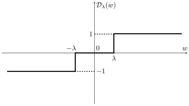
Figure 1: Dead-zone function $\operatorname{{\mathcal{D}}}_{\lambda}(w)$

If ${\boldsymbol{g}}_{i}({\boldsymbol{x}}^{\ast})^{\top}{\boldsymbol{p}}^{\ast}$ is equal to $-\lambda_{i}$ or $\lambda_{i}$ over a non-zero time interval, say $[t_{1},t_{2}]\subset[0,T]$, $t_{1}<t_{2}$, then the control $u_{i}$ (and hence ${\boldsymbol{u}}$) over $[t_{1},t_{2}]$ cannot be uniquely determined by the minimum principle. In this case, the interval $[t_{1},t_{2}]$ is called a singular interval, and a control problem that has at least one singular interval is called singular. If there is no singular interval, the problem is called normal:

Definition 4 (Normality)

The $L^{1}$-optimal control problem stated in Problem 2 is said to be normal if the set

$${\mathcal{T}}_{i}\triangleq\{t\in[0,T]:|\lambda_{i}^{-1}{\boldsymbol{g}}_{i}({\boldsymbol{x}}^{\ast}(t))^{\top}{\boldsymbol{p}}^{\ast}(t)|=1\}$$

is countable for $i=1,\dots,m$. If the problem is normal, the elements $t_{1},t_{2},\dots\in{\mathcal{T}}_{i}$ are called the switching times for the control $u_{i}(t)$. $\Box$

If the problem is normal, the components of the $L^{1}$-optimal control ${\boldsymbol{u}}^{\ast}(t)$ are piecewise constant and ternary, taking values $\pm 1$ or $0$ at almost all $t\in[0,T]$. This property, named ”bang-off-bang,” is key to connect the $L^{1}$-optimal control and the maximum-hands-off control as discussed in the next section.

5 Maximum-Hands-Off Control and $L^{1}$-Optimal Control

In this section, we consider a theoretical relation between maximum-hands-off control (Problem 1) and $L^{1}$-optimal control (Problem 2). The theorem below rationalizes the $L^{1}$ optimality in computing the maximum-hands-off control.

Theorem 5

Assume that the $L^{1}$-optimal control problem stated in Problem 2 is normal and has at least one solution. Let ${\mathcal{U}}_{0}^{\ast}$ and ${\mathcal{U}}_{1}^{\ast}$ be the sets of the optimal solutions of Problem 1 ($L^{0}$-optimal control problem) and Problem 2 ($L^{1}$-optimal control problem) respectively. Then we have ${\mathcal{U}}_{0}^{\ast}={\mathcal{U}}_{1}^{\ast}$.

Proof. Let ${\mathcal{U}}$ be the set of all admissible controls for the $L^{1}$-optimal control problem (Problem 2). By assumption, ${\mathcal{U}}_{1}^{\ast}$ is non-empty, and so is ${\mathcal{U}}$. The set ${\mathcal{U}}$ is also the admissible control set for the $L^{0}$-optimal control problem (Problem 1), and hence ${\mathcal{U}}_{0}^{\ast}\subset{\mathcal{U}}$. We first show that ${\mathcal{U}}_{0}^{\ast}$ is non-empty, and then prove ${\mathcal{U}}_{0}^{\ast}={\mathcal{U}}_{1}^{\ast}$.

First, for any ${\boldsymbol{u}}\in{\mathcal{U}}$, we have

$$\begin{split}J_{1}({\boldsymbol{u}})&=\sum_{i=1}^{m}\lambda_{i}\int_{0}^{T}|u_{i}(t)|~{}dt\\ &=\sum_{i=1}^{m}\lambda_{i}\int_{\operatorname*{supp}(u_{i})}|u_{i}(t)|~{}dt\\ &\leq\sum_{i=1}^{m}\lambda_{i}\int_{\operatorname*{supp}(u_{i})}1~{}dt=J_{0}({\boldsymbol{u}}).\end{split}$$ (9)

Now take an arbitrary ${\boldsymbol{u}}^{\ast}_{1}\in{\mathcal{U}}_{1}^{\ast}$. Since the problem is normal by assumption, each control $u_{1i}^{\ast}(t)$ in ${\boldsymbol{u}}_{1}^{\ast}(t)$ takes values $-1$, $0$, or $1$, at almost all $t\in[0,T]$. This implies that

$$\begin{split}J_{1}({\boldsymbol{u}}^{\ast}_{1})&=\sum_{i=1}^{m}\lambda_{i}\int_{0}^{T}|u_{1i}^{\ast}(t)|~{}dt\\ &=\sum_{i=1}^{m}\lambda_{i}\int_{\operatorname*{supp}(u_{1i}^{\ast})}1~{}dt=J_{0}({\boldsymbol{u}}^{\ast}_{1}).\end{split}$$ (10)

From (9) and (10), ${\boldsymbol{u}}^{\ast}_{1}$ is a minimizer of $J_{0}$, that is, ${\boldsymbol{u}}_{1}^{\ast}\in{\mathcal{U}}_{0}^{\ast}$. Thus, ${\mathcal{U}}_{0}^{\ast}$ is non-empty and ${\mathcal{U}}_{1}^{\ast}\subset{\mathcal{U}}_{0}^{\ast}$.

Conversely, let ${\boldsymbol{u}}^{\ast}_{0}\in{\mathcal{U}}_{0}^{\ast}\subset{\mathcal{U}}$. Take independently ${\boldsymbol{u}}^{\ast}_{1}\in{\mathcal{U}}_{1}^{\ast}\subset{\mathcal{U}}$. From (10) and the optimality of ${\boldsymbol{u}}^{\ast}_{1}$, we have

$$J_{0}({\boldsymbol{u}}^{\ast}_{1})=J_{1}({\boldsymbol{u}}^{\ast}_{1})\leq J_{1}({\boldsymbol{u}}^{\ast}_{0}).$$ (11)

On the other hand, from (9) and the optimality of ${\boldsymbol{u}}^{\ast}_{0}$, we have

$$J_{1}({\boldsymbol{u}}^{\ast}_{0})\leq J_{0}({\boldsymbol{u}}^{\ast}_{0})\leq J_{0}({\boldsymbol{u}}^{\ast}_{1}).$$ (12)

It follows from (11) and (12) that $J_{1}({\boldsymbol{u}}^{\ast}_{1})=J_{1}({\boldsymbol{u}}^{\ast}_{0})$, and hence ${\boldsymbol{u}}^{\ast}_{0}$ achieves the minimum value of $J_{1}$. That is, ${\boldsymbol{u}}_{0}^{\ast}\in{\mathcal{U}}_{1}^{\ast}$ and ${\mathcal{U}}_{0}^{\ast}\subset{\mathcal{U}}_{1}^{\ast}$. $\Box$

Theorem 5 suggests that $L^{1}$ optimization can be used for the maximum-hands-off (or the sparsest) solution. This is analogous to the situation in compressed sensing, where $L^{1}$ optimality is often used to obtain the sparsest vector; see [9, 10, 11] for details.

6 $L^{1}$/$L^{2}$-Optimal Control

In the previous section, we have shown that the maximum-hands-off control problem can be solved via $L^{1}$-optimal control. From the ”bang-off-bang” property of the $L^{1}$-optimal control, the control changes its value at switching times discontinuously. This is undesirable for some applications in which the actuators cannot move abruptly. In this case, one may want to make the control continuous. For this purpose, we add a regularization term to the $L^{1}$ cost $J_{1}({\boldsymbol{u}})$ defined in (6). More precisely, we consider the following mixed $L^{1}$/$L^{2}$-optimal control problem.

Problem 6 ($L^{1}$/$L^{2}$-Optimal Control)

Find an admissible control $\{{\boldsymbol{u}}(t):t\in[0,T]\}\in{\mathcal{U}}$ that minimizes

$$\begin{split}J_{12}({\boldsymbol{u}})&\triangleq\sum_{i=1}^{m}\biggl{(}\lambda_{i}\|u_{i}\|_{L^{1}}+\frac{1}{2}r_{i}\|u_{i}\|_{L^{2}}^{2}\biggr{)}\\ &=\int_{0}^{T}\sum_{i=1}^{m}\biggl{(}\lambda_{i}|u_{i}(t)|+\frac{1}{2}r_{i}|u_{i}(t)|^{2}\biggr{)}dt,\end{split}$$ (13)

where $\lambda_{i}>0$ and $r_{i}>0$, $i=1,\dots,m$, are given weights.

To discuss the optimal solution(s) of the above problem, we next give necessary conditions for the $L^{1}$/$L^{2}$-optimal control using the minimum principle of Pontryagin.

The Hamiltonian function is given by

$$\begin{split}H({\boldsymbol{x}},{\boldsymbol{p}},{\boldsymbol{u}})&=\sum_{i=1}^{m}\biggl{(}\lambda_{i}|u_{i}|+\frac{1}{2}r_{i}|u_{i}|^{2}\biggr{)}\\ &\quad+{\boldsymbol{p}}^{\top}\biggl{(}{\boldsymbol{f}}({\boldsymbol{x}})+\sum_{i=1}^{m}{\boldsymbol{g}}_{i}({\boldsymbol{x}})u_{i}\biggr{)}\end{split}$$

where ${\boldsymbol{p}}$ is the costate vector. Let ${\boldsymbol{u}}^{\ast}$ denote the optimal control and ${\boldsymbol{x}}^{\ast}$ and ${\boldsymbol{p}}^{\ast}$ the resultant optimal state and costate, respectively. Then we have the following result.

Lemma 7

The $i$-th element $u_{i}^{\ast}(t)$ of the $L^{1}$/$L^{2}$-optimal control ${\boldsymbol{u}}^{\ast}(t)$ satisfies

$$u_{i}^{\ast}(t)=-\operatorname{sat}\left\{\operatorname{{\mathcal{S}}}_{\lambda_{i}/r_{i}}\left(r_{i}^{-1}{\boldsymbol{g}}_{i}\bigl{(}{\boldsymbol{x}}^{\ast}(t)\bigr{)}^{\top}{\boldsymbol{p}}^{\ast}(t)\right)\right\},$$ (14)

where $\operatorname{{\mathcal{S}}}_{\lambda/r}(\cdot)$ is the shrinkage function defined by

$$\operatorname{{\mathcal{S}}}_{\lambda/r}(v)\triangleq\begin{cases}v+\lambda/r&{\rm{if~{}}}v<-\lambda/r,\\ 0,&{\rm{if~{}}}-\lambda/r\leq v\leq\lambda/r,\\ v-\lambda/r,&{\rm{if~{}}}\lambda/r<v,\\ \end{cases}$$

and $\operatorname{sat}(\cdot)$ is the saturation function defined by

$$\operatorname{sat}(v)\triangleq\begin{cases}-1,&\text{\rm if~{}}v<-1,\\ v,&\text{\rm if~{}}-1\leq v\leq 1,\\ 1,&\text{\rm if~{}}1<v.\\ \end{cases}$$

See Figs. 2 and 3 for the graphs of $\operatorname{{\mathcal{S}}}_{\lambda/r}(\cdot)$ and $\operatorname{sat}\!\left(\operatorname{{\mathcal{S}}}_{\lambda/r}(\cdot)\right)$, respectively.

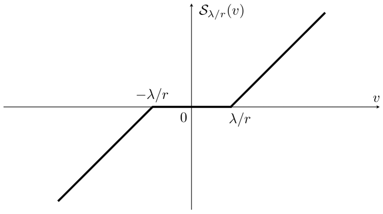
Figure 2: Shrinkage function $\operatorname{{\mathcal{S}}}_{\lambda/r}(v)$

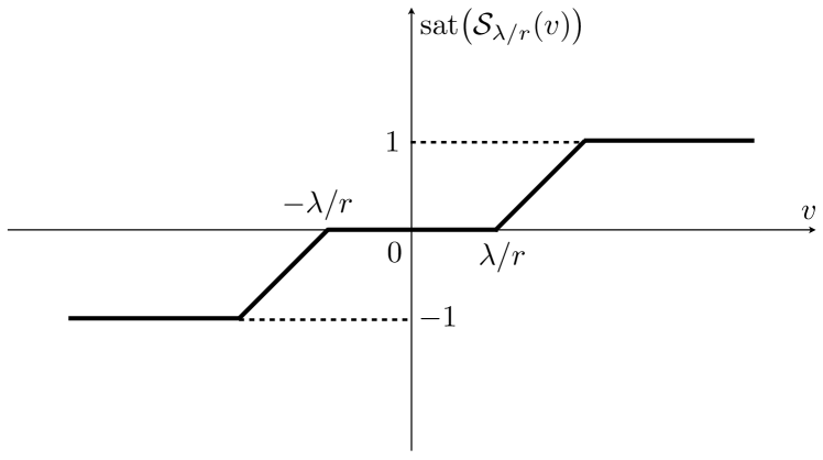
Figure 3: Saturated shrinkage function $\operatorname{sat}\!\left(\operatorname{{\mathcal{S}}}_{\lambda/r}(v)\right)$

Proof. The result is easily obtained from the fact that

$$-\operatorname{sat}\left\{\operatorname{{\mathcal{S}}}_{\lambda/r}\left(r^{-1}a\right)\right\}=\operatorname*{arg\,min}_{|u|\leq 1}\lambda|u|+\frac{1}{2}r|u|^{2}+au,$$

for any $\lambda>0$, $r>0$, and $a\in\mathbb{R}$. $\Box$

From Lemma 7, we have the following proposition.

Proposition 8 (Continuity)

The $L^{1}$/$L^{2}$-optimal control ${\boldsymbol{u}}^{\ast}(t)$ is continuous in $t$ over $[0,T]$.

Proof. Without loss of generality, we assume $m=1$ (a single input plant), and omit subscripts for $u$, $r$, $\lambda$, and so on. Let

$$\bar{u}({\boldsymbol{x}},{\boldsymbol{p}})\triangleq-\operatorname{sat}\left\{\operatorname{{\mathcal{S}}}_{\lambda/r}\left(r^{-1}{\boldsymbol{g}}_{i}({\boldsymbol{x}})^{\top}{\boldsymbol{p}}\right)\right\}.$$

Since functions $\left(\operatorname{sat}\circ\operatorname{{\mathcal{S}}}_{\lambda/r}\right)(\cdot)$ and ${\boldsymbol{g}}(\cdot)$ are continuous, $\bar{u}({\boldsymbol{x}},{\boldsymbol{p}})$ is also continuous in ${\boldsymbol{x}}$ and ${\boldsymbol{p}}$. It follows from Lemma 7 that the optimal control $u^{\ast}$ given in (14) is continuous in ${\boldsymbol{x}}^{\ast}$ and ${\boldsymbol{p}}^{\ast}$. Hence, $u^{\ast}(t)$ is continuous if ${\boldsymbol{x}}^{\ast}(t)$ and ${\boldsymbol{p}}^{\ast}(t)$ are continuous in $t$ over $[0,T]$.

The canonical system for the $L^{1}$/$L^{2}$-optimal control is given by

$$\begin{split}\frac{d{\boldsymbol{x}}^{\ast}(t)}{dt}&={\boldsymbol{f}}\bigl{(}{\boldsymbol{x}}^{\ast}(t)\bigr{)}+{\boldsymbol{g}}\bigl{(}{\boldsymbol{x}}^{\ast}(t)\bigr{)}\bar{u}\bigl{(}{\boldsymbol{x}}^{\ast}(t),{\boldsymbol{p}}^{\ast}(t)\bigr{)},\\ \frac{d{\boldsymbol{p}}^{\ast}(t)}{dt}&=-{\boldsymbol{f}}^{\prime}\bigl{(}{\boldsymbol{x}}^{\ast}(t)\bigr{)}^{\top}{\boldsymbol{p}}^{\ast}(t)\\ &\qquad-\bar{u}\bigl{(}{\boldsymbol{x}}^{\ast}(t),{\boldsymbol{p}}^{\ast}(t)\bigr{)}{\boldsymbol{g}}^{\prime}\bigl{(}{\boldsymbol{x}}^{\ast}(t)\bigr{)}^{\top}{\boldsymbol{p}}^{\ast}(t).\end{split}$$

Since ${\boldsymbol{f}}({\boldsymbol{x}})$, ${\boldsymbol{g}}({\boldsymbol{x}})$, ${\boldsymbol{f}}^{\prime}({\boldsymbol{x}})$, and ${\boldsymbol{g}}^{\prime}({\boldsymbol{x}})$ are continuous in ${\boldsymbol{x}}$ by assumption, and so is $\bar{u}({\boldsymbol{x}},{\boldsymbol{p}})$ in ${\boldsymbol{x}}$ and ${\boldsymbol{p}}$, the right hand side of the canonical system is continuous in ${\boldsymbol{x}}^{\ast}$ and ${\boldsymbol{p}}^{\ast}$. From a continuity theorem of dynamical systems, e.g. [3, Theorem 3-14], it follows that the resultant trajectories ${\boldsymbol{x}}^{\ast}(t)$ and ${\boldsymbol{p}}^{\ast}(t)$ are continuous in $t$ over $[0,T]$. $\Box$

Proposition 8 motivates us to use $L^{1}/L^{2}$ optimization as in Problem 6 for continuous hands-off control.

In general, the degree of continuity (or smoothness) and the sparsity of the control input cannot be optimized at the same time. Then, the weights $\lambda_{i}$ or $r_{i}$ can be used for trading smoothness for sparsity. From Lemma 7, increasing the weight $\lambda_{i}$ (or decreasing $r_{i}$) makes the $i$-th input $u_{i}(t)$ sparser (see also Fig. 3). On the other hand, decreasing $\lambda_{i}$ (or increasing $r_{i}$) smoothens $u_{i}(t)$. Moreover, we have the following limiting properties.

Proposition 9 (Limiting property)

Assume the $L^{1}$-optimal control problem is normal. Let ${\boldsymbol{u}}_{1}({\boldsymbol{\lambda}})$ and ${\boldsymbol{u}}_{12}({\boldsymbol{\lambda}},{\boldsymbol{r}})$ be solutions to respectively Problems 2 and 6 with parameters

$${\boldsymbol{\lambda}}\triangleq(\lambda_{1},\dots,\lambda_{m}),\quad{\boldsymbol{r}}\triangleq(r_{1},\dots,r_{m}).$$

For any fixed ${\boldsymbol{\lambda}}>0$, we have

$$\lim_{{\boldsymbol{r}}\rightarrow{\boldsymbol{0}}}{\boldsymbol{u}}_{12}({\boldsymbol{\lambda}},{\boldsymbol{r}})={\boldsymbol{u}}_{1}({\boldsymbol{\lambda}}).$$

Moreover, for any fixed ${\boldsymbol{r}}>0$, we have

$$\lim_{{\boldsymbol{\lambda}}\rightarrow{\boldsymbol{0}}}{\boldsymbol{u}}_{12}({\boldsymbol{\lambda}},{\boldsymbol{r}})={\boldsymbol{u}}_{2}({\boldsymbol{r}}),$$

where ${\boldsymbol{u}}_{2}({\boldsymbol{r}})$ is an $L^{2}$-optimal (or minimum-energy) control discussed in [3, Chap. 6], that is, a solution to a control problem where $J_{1}({\boldsymbol{u}})$ in Problem 2 is replaced with

$$J_{2}({\boldsymbol{u}})=\int_{0}^{T}\sum_{i=1}^{m}\frac{1}{2}r_{i}|u_{i}(t)|^{2}dt.$$ (15)

Proof. The first statement follows directly from the fact that for any fixed $\lambda>0$, we have

$$\lim_{r\rightarrow 0}\operatorname{sat}\!\left({\mathcal{S}}_{\lambda/r}(r^{-1}w)\right)=\operatorname{{\mathcal{D}}}_{\lambda}(w),\quad\forall w\in\mathbb{R}\setminus\{\pm\lambda\},$$

where $\operatorname{{\mathcal{D}}}_{\lambda}(\cdot)$ is the dead-zone function defined in (8). The second statement derives from the fact that for any fixed $r>0$, we have

$$\lim_{\lambda\rightarrow 0}\operatorname{sat}\!\left({\mathcal{S}}_{\lambda/r}(v)\right)=\operatorname{sat}(v),\quad\forall v\in\mathbb{R}.$$

$\Box$

In summary, the $L^{1}$/$L^{2}$-optimal control is an intermediate control between the $L^{1}$-optimal control (or the maximum-hands-off control) and the $L^{2}$-optimal control.

7 Examples

We here consider the following 4th order system:

$$\frac{d{\boldsymbol{x}}(t)}{dt}=\begin{bmatrix}0&-1&0&0\\ 1&0&0&0\\ 0&1&0&0\\ 0&0&1&0\end{bmatrix}{\boldsymbol{x}}(t)+\begin{bmatrix}2\\ 0\\ 0\\ 0\end{bmatrix}u(t).$$

We set the final time $T=10$, and the initial and final states as

$${\boldsymbol{x}}(0)=[1,1,1,1]^{\top},\quad{\boldsymbol{x}}(10)={\boldsymbol{0}}.$$

Note that the system has poles at $s=0$, $0$, $\pm j$.

We first compute the maximum-hands-off control with $L^{1}$-optimal control as discussed in Section 5. We compute the optimal control input by a time discretization method, see e.g., [16, Sec. 2.3]. Fig. 4 shows the obtained control. The figure also shows the $L^{2}$-optimal control that minimizes $J_{2}(u)$ in (15) with $r_{1}=1$. We can see that the maximum-hands-off control is quite sparse. In fact, we have

$$\|u\|_{L^{0}}=1.92\text{~{}(sec)},$$

which is $19.2$% out of $10$ (sec). In other words, the control keeps hands-off over $80.8$% of the control period. On the other hand, the $L^{2}$ optimal control is not sparse, while its energy, $J_{2}(u)$, is smaller than that of maximum-hands-off control.

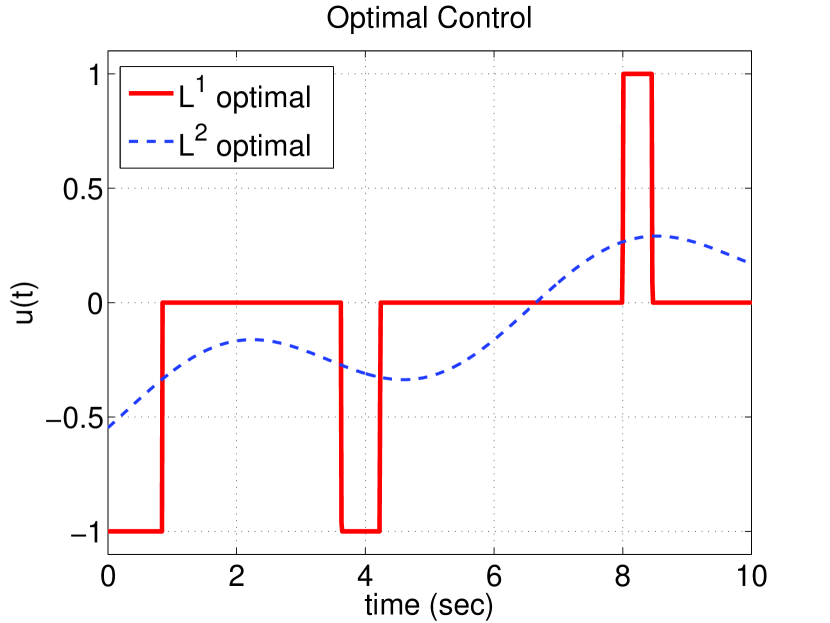
Figure 4: Maximum-hands-off control via $L^{1}$ optimization (solid) and $L^{2}$ optimal control (dashed).

Fig. 5 shows the state variables $x_{1}(t)$, $x_{2}(t)$, $x_{3}(t)$, and $x_{4}(t)$ along with the maximum-hands-off control $u(t)$ over time interval $[0,10]$.

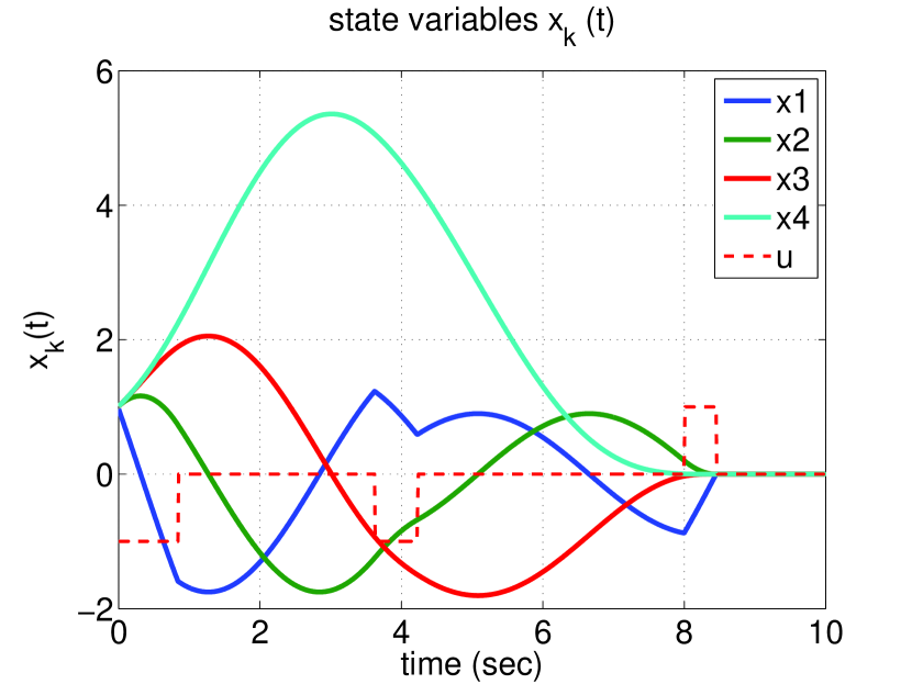
Figure 5: Maximum-hands-off control: state variables $x_{1}(t),\dots,x_{4}(t)$ (solid) and input $u(t)$ (dashed)

We can see that the states almost stay at the origin after the last switching time, $t=8.47$ (sec).

We next consider the $L^{1}$/$L^{2}$-optimal control method proposed in Section 6. We use the same parameters as above. The weights $\lambda_{1}$ and $r_{1}$ in (13) are chosen as $\lambda_{1}=r_{1}=1$. We solve the optimal control problem via a time discretization method. Fig. 6 shows the obtained $L^{1}$/$L^{2}$-optimal control. The figure also shows the maximum-hands-off control obtained above.

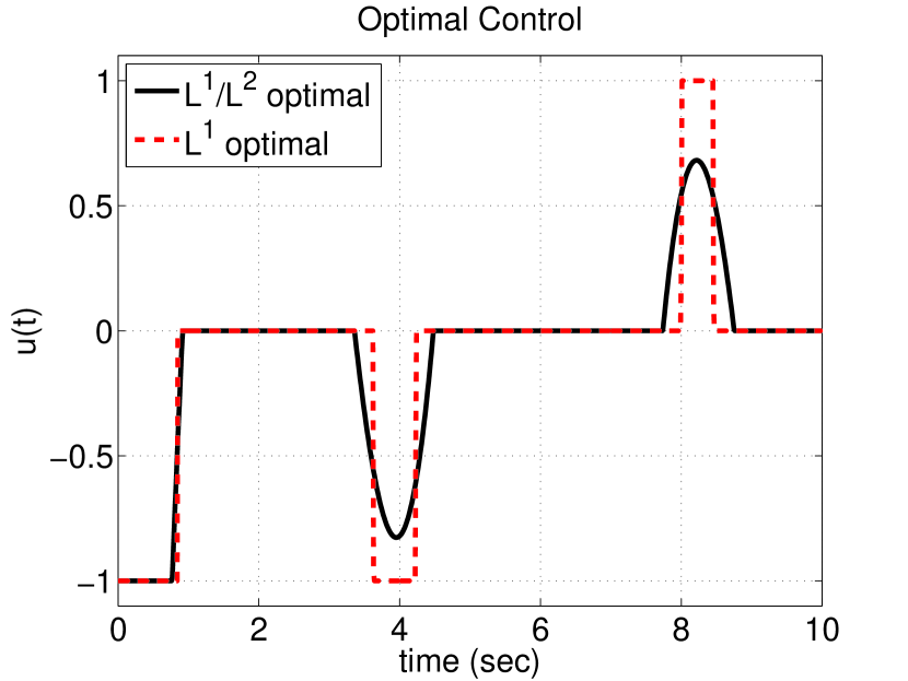
Figure 6: $L^{1}$/$L^{2}$-optimal control (solid) and maximum-hands-off control (dash).

We can see that the $L^{1}$/$L^{2}$-optimal control is continuous while the maximum-hands-off control exhibits the ”bang-off-bang” property. On the other hand, the $L^{1}$/$L^{2}$-optimal control has a longer support than the $L^{1}$-optimal control. To see the tradeoff property between sparsity and smoothness of control, we compute the $L^{0}$ norm, $\|u\|_{L^{0}}$, and the $L^{\infty}$ norm of the derivative of $u(t)$, that is,

$$\left\|\frac{du(t)}{dt}\right\|_{L^{\infty}}\triangleq\sup_{t\in[0,T]}\left|\frac{du(t)}{dt}\right|,$$

as a function of $r_{1}$ while $\lambda_{1}$ is fixed to be $1$. Fig. 7 shows the result.

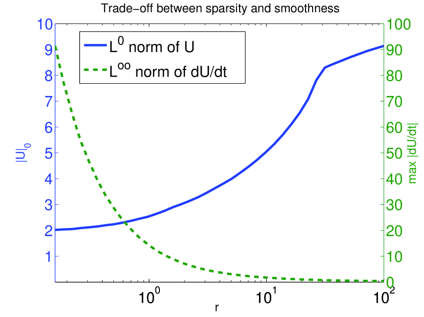
Figure 7: $L^{0}$ norm of $u(t)$ (solid) and $L^{\infty}$ norm of $du/dt$ (dash) versus weight $r$.

We can see that the weight $r$ can take account of the tradeoff between sparsity and smoothness in hands-off control.

8 Conclusion

In this article, we have presented maximum-hands-off control and shown that it is $L^{1}$ optimal. This shows that efficient optimization methods for $L^{1}$ problems can be used to obtain maximum-hands-off control. We have also proposed an $L^{1}$/$L^{2}$-optimal control to obtain smooth hands-off control, while the maximum-hands-off control is discontinuous due to the ”bang-off-bang” property. Numerical examples show the effectiveness of the proposed control. Future work may include adaptation of hands-off control to sparsely packetized predictive control as in [14, 15].

References

[1]
B. D. O. Anderson and J. B. Moore, Optimal Filtering. Dover Publications, 2005.
[2]
M. Athans, “Minimum-fuel feedback control systems: second-order case,”
IEEE Trans. Appl. Ind., vol. 82, pp. 8–17, 1963.
[3]
M. Athans and P. L. Falb, Optimal Control. Dover Publications, 1966.
[4]
W. Brockett, “Minimum attention control,” in 36th IEEE Conference on
Decision and Control (CDC), vol. 3, Dec. 1997, pp. 2628–2632.
[5]
E. J. Candes, “Compressive sampling,” Proc. International Congress of
Mathematicians, vol. 3, pp. 1433–1452, Aug. 2006.
[6]
C. Chan, “The state of the art of electric, hybrid, and fuel cell vehicles,”
Proc. IEEE, vol. 95, no. 4, pp. 704–718, Apr. 2007.
[7]
D. L. Donoho, “Compressed sensing,” IEEE Trans. Inf. Theory,
vol. 52, no. 4, pp. 1289–1306, Apr. 2006.
[8]
B. Dunham, “Automatic on/off switching gives 10-percent gas saving,”
Popular Science, vol. 205, no. 4, p. 170, Oct. 1974.
[9]
M. Elad, Sparse and Redundant Representations. Springer, 2010.
[10]
Y. C. Eldar and G. Kutyniok, Compressed Sensing: Theory and
Applications. Cambridge University
Press, 2012.
[11]
K. Hayashi, M. Nagahara, and T. Tanaka, “A user’s guide to compressed sensing
for communications systems,” IEICE Trans. on Communications, vol.
E96-B, no. 3, pp. 685–712, Mar. 2013.
[12]
D. Jeong and W. Jeon, “Performance of adaptive sleep period control for
wireless communications systems,” IEEE Trans. Wireless Commun.,
vol. 5, no. 11, pp. 3012–3016, Nov. 2006.
[13]
L. Kong, G. Wong, and D. Tsang, “Performance study and system optimization on
sleep mode operation in IEEE 802.16e,” IEEE Trans. Wireless
Commun., vol. 8, no. 9, pp. 4518–4528, Sep. 2009.
[14]
M. Nagahara and D. E. Quevedo, “Sparse representations for packetized
predictive networked control,” in IFAC 18th World Congress, Sep.
2011, pp. 84–89.
[15]
M. Nagahara, D. E. Quevedo, and J. Østergaard, “Packetized predictive
control for rate-limited networks via sparse representation,” in 51st
IEEE Conference on Decision and Control (CDC), Dec. 2012, pp. 1362–1367.
[16]
R. F. Stengel, Optimal Control and Estimation. Dover Publications, 1994.
[17]
T. Tao, An Epsilon of Room, I: Real Analysis. AMS, Feb. 2011.