Magnetic Susceptibility of Strongly Interacting Matter across the Deconfinement Transition

Abstract

We propose a method to determine the total magnetic susceptibility of strongly interacting matter by lattice QCD simulations, and present first numerical results for the theory with two light flavors, which suggest a weak magnetic activity in the confined phase and the emergence of strong paramagnetism in the deconfined, Quark-Gluon Plasma phase.

Introduction – Understanding the properties of strong interactions in the presence of strong magnetic backgrounds is a problem of the utmost phenomenological importance. The physics of compact astrophysical objects, like magnetars magnetars , of non-central heavy ion collisions hi1 ; hi2 ; hi3 ; hi4 and of the early Universe vacha ; grarub , involvs fields going from $10^{10}$ Tesla up to $10^{15-16}$ Tesla ($|e|B\sim 1$ GeV²). The problem is also relevant to a better comprehension of the non-perturbative properties of QCD and of the Stardard Model in general. That justifies the recent theoretical efforts on the subject (see, e.g., Ref. lecnotmag ).

Any material is characterized by the way it reacts to electromagnetic external sources. For strongly interacting matter, such as that present in the early Universe and in the core of compact astrophysical objects, or that created in heavy ion collisions, the same questions as for any other medium can be posed. Does it react linearly to magnetic backgrounds, at least for small fields, and is it a paramagnet or a diamagnet? How the magnetic susceptibility $\chi$ changes as a function of the temperature $T$ and/or chemical potentials?

Despite the clear-cut nature of such questions, a definite answer is still missing. Strong interactions in external fields can be conveniently explored by lattice QCD simulations; various investigations have focussed till now on partial aspects, like the magnetic properties of the spin component buivid ; reg1 and of the QCD vacuum reg2 . Most technical difficulties are related to the fact that in a lattice setup, which usually adopts toroidal geometries, the magnetic background is quantized.

In the following we propose a new method to overcome such difficulties and present a first investigation for QCD with 2 light flavors in the standard rooted staggered formulation, performed at various values of the lattice spacing $a$ and of the quark masses. Results show that $\chi$ is small (vanishing within present errors) in the confined phase, while it steeply rises above the transition, i.e. the Quark-Gluon Plasma is paramagnetic.

The method – The magnetic properties of a homogeneous medium at thermal equilibrium can be inferred from the change of its free energy density, $f=F/V$, in terms of an applied constant and uniform field:

$$\Delta f(B,T)=-\frac{T}{V}\log\left(\frac{Z(B,T,V)}{Z(0,T,V)}\right)$$ (1)

where $Z=\exp(-F/T)$ is the partition function of the system, $B$ is the magnetic field modulus and $V$ is the spatial volume. One usually deals directly with free energy derivatives, like the magnetization, which can be rewritten in terms of thermal expectation values and are extracted more easily than free energy differences, whose computation is notoriously difficult (see, e.g., Ref. umbrella ).

However, in lattice simulations the best way to deal with a finite spatial volume, while minimizing finite size effects and keeping a homogeneous background field, is to work on a compact manifold without boundaries, such as a 3D torus (cubic lattice with periodic boundary conditions). That leads to ambiguities in the presence of charged particles moving over the manifold, unless the total flux of the magnetic field, across a section orthogonal to it, is quantized in units of $2\pi/q$, where $q$ is the elementary electric particle charge. The same argument leads to Dirac quantization of the magnetic monopole charge, when considering a spherical surface around it. In the case of the 3D torus, assuming $\bm{B}=B\ \bm{\hat{z}}$ and considering that for quarks $q=|e|/3$, one has bound1 ; bound2 ; bound3 ; wiese

$$|e|B={6\pi b}/{(l_{x}l_{y})}$$ (2)

where $b$ is an integer and $l_{x}$, $l_{y}$ are the torus extensions in the $x,y$ directions.

Since $B$ is quantized, taking derivatives with respect to it is not well defined. New approaches can be found to get around the problem, like the anisotropy method reg2 . However, one can still go back to Eq. (1) and consider finite free energy differences: this is our strategy, as explained in the following. Let us first recall more details regarding the magnetic field on the lattice torus.

Electromagnetic fields enter the QCD lagrangian through the covariant derivative of quarks, $D_{\mu}=\partial_{\mu}+i\,gA^{a}_{\mu}T^{a}+i\,qA_{\mu}$, where $A_{\mu}$ is the electromagnetic gauge potential and $q$ is the quark electric charge. On the lattice, that corresponds to adding proper $U(1)$ phases $u_{\mu}(n)$ to the $SU(3)$ parallel transports entering the discretized Dirac operator, $U_{\mu}(n)\to u_{\mu}(n)U_{\mu}(n)$, where $n$ is a lattice site. A magnetic field $\bm{B}=B\ \bm{\hat{z}}$ can be realized, for instance, by a potential $A_{y}=Bx$ and $A_{\mu}=0\ {\rm for}\ \mu\neq y$. In the presence of periodic boundary conditions, $B$ must be quantized as in Eq. (2) and proper b.c. must be chosen for fermions, to preserve gauge invariance wiese . The corresponding $U(1)$ links are

$$u_{y}^{(q)}(n) =e^{i\,a^{2}qB\,n_{x}} = \ e^{i\,2\pi b\,n_{x}/(L_{x}L_{y})}$$ (3)

$$u_{x}^{(q)}(n)|_{n_{x}=L_{x}} =e^{-i\,a^{2}qL_{x}B\,n_{y}} = \ e^{-i\,2\pi b\,n_{y}/L_{y}}$$

and $u_{\nu}(n)=1$ otherwise, where $n_{\mu}\in\{1,\ldots,L_{\mu}\}$, $L_{\mu}$ being the lattice extension along $\mu$; $b$ gets a factor -2 for $u$ quarks with respect to $d$ quarks.

With this choice, a constant magnetic flux $a^{2}B$ goes through all plaquettes in the $xy$ plane, apart from a “singular” plaquette located at $n_{x}=L_{x}$ and $n_{y}=L_{y}$, which is pierced by a flux $(1-L_{x}L_{y})a^{2}B$, leading to a vanishing total flux through the $xy$ torus, as expected for a closed surface. In the continuum limit, that corresponds to a uniform magnetic field plus a Dirac string piercing the torus in one point: like for Dirac monopoles, the string carries all the flux away. However, if $B$ is quantized as in Eq. (2), the string becomes invisible to all particles carrying electric charges multiple of $q$, and the phase of the singular plaquette becomes equivalent, modulo $2\pi$, to that of all other plaquettes, i.e. the field is uniform.

Consider now the problem of computing finite free energy differences, $f(B_{2})-f(B_{1})=f(b_{2})-f(b_{1})$ where $b_{1}$ and $b_{2}$ are integers. Several methods are known to determine such differences in an efficient way (see, e.g., Ref. thooft ): the general idea is to divide them into a sum of smaller, easily computable differences. We will consider infinitesimal differences and rewrite

$$f(b_{2})-f(b_{1})=\int_{b_{1}}^{b_{2}}\frac{\partial f(b)}{\partial b}\mathrm{d}b\,,$$ (4)

the idea being to determine the integral after computing the integrand on a grid of points, fine enough to keep systematic errors under control.

Let us clarify the meaning of $\partial f/\partial b$. Generic real values of $b$ correspond to a uniform field plus a visible Dirac string: while this is not the physical situation we are interested in, it still represents a legitimate theory, interpolating between integer values of $b$. In practice, we are extending a function, originally defined on integers, to the real axis, and then we are integrating its derivative, $\partial f/\partial b$, between integer values to recover the original function: as long as the extension is analytic, as always possible on a finite lattice, the operation is well defined (see the Appendix for an explicit check).

Therefore, ${\partial f}/{\partial b}$ has no direct relation with the magnetization, even for integer $b$. For the particular interpolation adopted, a large contribution to it comes from the string itself, leading to a characteristic oscillating behavior; since $f(b)$ has a local minimum when the string becomes invisible, ${\partial f}/{\partial b}$ vanishes for integer $b$.

Renormalization – The procedure described above gives access to $\Delta f(B,T)$, defined in Eq. (1), however we have to take care of divergent contributions. Indeed, $B$-dependent divergences do not cancel when taking the difference $\Delta f$, and must be properly subtracted, with possible ambiguities related to the definition of the vacuum energy in the presence of a magnetic field. For $T=0$, the prescription of Ref. reg2 is to subtract all terms quadratic in $B$, so that, by definition, the magnetic properties of the QCD vacuum are of higher order in $B$.

In the following, we are not interested in the magnetic properties of vacuum, but only in those of the strongly interacting thermal medium, which may be probed experimentally. Therefore, our prescription is to compute the following quantity:

$$\Delta f_{R}(B,T)=\Delta f(B,T)-\Delta f(B,0)$$ (5)

which is properly renormalized, since all vacuum (zero $T$) contributions have been subtracted and no further divergences, depending both on $B$ and on $T$, appear (see, e.g., the discussion in Refs. reg0 ; reg2 ). Clearly, divergences are really removed only if the contributions to Eq. (5) are evaluated at a fixed value of the lattice spacing. The small field behavior of $\Delta f_{R}$ will give access to the magnetic susceptibility of the medium.

Effects of QED quenching – For small fields and for a linear, homogeneous and isotropic medium, the magnetization $\bm{\mathcal{M}}$ is proportional to the total field $\bm{B}$ acting on the medium, $\bm{\mathcal{M}}=\tilde{\chi}\bm{B}/\mu_{0}$ (using SI units), where $\tilde{\chi}$ is the susceptibility. The relation can also be expressed as $\bm{\mathcal{M}}=\chi\bm{H}$, where $\bm{H}=\bm{B}/\mu_{0}-\bm{\mathcal{M}}$ and the relation $\chi=\tilde{\chi}/(1-\tilde{\chi})$ holds between the two different definitions of susceptibility.

The change in the free energy density is usually written in the form $\Delta f=\int\bm{H}\cdot\mathrm{d}\bm{B}$ (see, e.g., Ref. LL §31). However, in $\Delta f_{R}$ the energy of the magnetic field alone is subtracted, hence the proper expression is: $\Delta f_{R}=-\int\bm{\mathcal{M}}\cdot\mathrm{d}\bm{B}$. Taking into account $\bm{\mathcal{M}}=\tilde{\chi}\bm{B}/\mu_{0}$ we get, in the limit of small fields,

$$\Delta f_{R}=-\frac{\tilde{\chi}}{\mu_{0}}\int\bm{B}\cdot\mathrm{d}\bm{B}=-\frac{\tilde{\chi}}{2\mu_{0}}\bm{B}^{2}\ \equiv-\frac{\hat{\chi}}{2}(e\bm{B})^{2}\ \,.$$ (6)

The field $\bm{B}$ in the last equation is the total field felt by the particles of the medium, i.e. that entering the Dirac matrix: since in our setup the dynamics of electromagnetic fields is quenched, it coincides with the external field added to the system, i.e. we do not have to add the field generated by the magnetization itself. Last quantity introduced in Eq. (6), $\hat{\chi}$, will be used for $\Delta f_{R}$ and $(eB)^{2}$ both measured in natural units.

$L_{s}$	$L_{t}$	$\beta$	$am$	$a$[fm]	$m_{\pi}$	$T$	$\tilde{\chi}\times 10^{3}$	$\hat{\chi}\times 10^{2}$
20	4	5.4075	0.00334	0.188	195	262	1.89(21)	2.06(23)
16	4	5.4342	0.00584	0.17	275	290	2.04(13)	2.22(15)
16	6	5.4342	0.00584	0.17	275	193	0.70(15)	0.76(16)
16	8	5.4342	0.00584	0.17	275	145	0.23(23)	0.25(25)
24	4	5.527	0.0146	0.141	480	349	2.69(20)	2.93(22)
24	6	5.527	0.0146	0.141	480	233	1.42(16)	1.55(18)
24	8	5.527	0.0146	0.141	480	175	0.49(21)	0.53(22)
24	10	5.527	0.0146	0.141	480	140	0.15(20)	0.16(22)
16	4	5.453	0.02627	0.188	480	262	1.54(10)	1.68(10)
16	6	5.453	0.02627	0.188	480	175	0.21(11)	0.23(12)
16	8	5.453	0.02627	0.188	480	131	0.05(11)	0.05(12)
16	4	5.3945	0.0495	0.24	480	205	0.51(7)	0.56(8)
16	8	5.3945	0.0495	0.24	480	103	0.00(8)	0.00(9)

Table 1: Lattice parameters and results. $T$ and $m_{\pi}$ are in MeV units, $\tilde{\chi}$ in SI units, while $\hat{\chi}$ for both $\Delta f_{R}$ and $(eB)^{2}$ measured in natural units (see Eq. (6)).

Numerical results – As a first application of our method, we consider $N_{f}=2$ QCD with fermions in the standard rooted staggered formulation, with each quark described by the fourth root of the fermion determinant. The partition function reads:

$$Z\equiv\int\mathcal{D}Ue^{-S_{G}}\det D^{1\over 4}[U,q_{u}]\det D^{1\over 4}[U,q_{d}]\>$$ (7)

$$D^{(q)}_{i,j}\equiv am\delta_{i,j} + {1\over 2}\sum_{\nu=1}^{4}\eta_{\nu}(i)\left(u_{\nu}^{(q)}(i)\ U_{\nu}(i)\delta_{i,j-\hat{\nu}}\right.$$ (8)

$$- \left.u^{*(q)}_{\nu}{(i-\hat{\nu})}\ U^{{\dagger}}_{\nu}{(i-\hat{\nu})}\delta_{i,j+\hat{\nu}}\right)\>$$

$\mathcal{D}U$ is the integration over $SU(3)$ gauge link variables, $S_{G}$ is the plaquette action, $i$, $j$ are lattice site indexes, $\eta_{\nu}(i)$ are the staggered phases. The quark charges are $q_{u}=2|e|/3$ and $q_{d}=-|e|/3$. The density of the integrand in Eq. (4) can be expressed as

$$M\equiv a^{4}\frac{\partial f}{\partial b}=\frac{1}{4L_{t}L_{s}^{3}}\sum_{q=u,d}\Big{\langle}\mbox{Tr}\Big{\{}\frac{\partial D^{(q)}}{\partial b}{D^{(q)}}^{-1}\Big{\}}\Big{\rangle}\,$$ (9)

where $L_{s}$ and $L_{t}$ are the temporal and spatial sizes ($T=1/(L_{t}a)$). We stress again that $M$ is just the derivative of the free energy interpolation and has no direct physical interpretation.

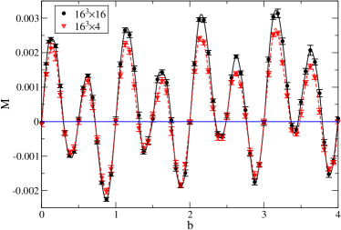
Figure 1: $M$ computed on $16^{4}$ and $16^{3}\times 4$ lattices, with $a\approx 0.188$ fm and $m_{\pi}\approx 480$ MeV. The lines are third order spline interpolations.

We have explored different lattice spacings and pseudo-Goldstone pion masses, by tuning the inverse gauge coupling $\beta$ and $am$ according to Ref. blum (the magnetic background does not modify $a$ reg0 ; thetaeff ), and different values of $L_{s}$ and $L_{t}$ (see Table 1). For the explored sets, the pseudocritical temperature $T_{c}$ is in the range 160-170 MeV demusa . We have adopted a Rational Hybrid Monte-Carlo (RHMC) algorithm implemented on GPU cards gpu , with statistics of $O(10^{3})$ molecular dynamics (MD) time units for each $b$. $M$ has been measured every 5 trajectories, of one MD time unit each, adopting a noisy estimator, with $10$ random vectors for each measure.

Fig. 1 shows an example of the determination of $M$, for the first 4 quanta of $B$, for one parameter set and for $L_{t}=4$ and $16$, the latter being taken as our $T\sim 0$ reference value. Oscillations between successive quanta can be related to the presence of the string: the two visible harmonics are associable with the $d$ and $u$ quark contributions, which feel the string differently.

Despite the unphysical oscillations, $M$ is smooth enough to perform a numerical integration: that is done by using a spline interpolation over 16 equally spaced determinations of $M$ for each quantum; errors are estimated by means of a bootstrap analysis. We checked that variations due to different integration schemes, or to different interpolating strategies and densities, always stay well within the estimated errors, so that the integration procedure is very robust (see the Appendix for details).

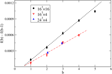
Figure 2: $f(b)-f(b-1)$ computed from data in Fig. 1, together with best fits obtained, for $b\leq 4$, according to $c_{2}\,(2b-1)$ (see Eq. (10)). Two further, properly rescaled data points are reported from a $24^{3}\times 4$ lattice.

To obtain the $\mathcal{O}(B^{2})$ term in $\Delta f_{R}(B,T)$, we have determined the $\mathcal{O}(B^{2})$ contributions to both $\Delta f(B,T)$ and $\Delta f(B,0)$, then we have subtracted them; consistent results are obtained if the subtraction is performed first. Assuming that $a^{4}\Delta f(b)\equiv c_{2}\,b^{2}+O(b^{4})$ holds for integer $b$, $c_{2}$ is conveniently determined by looking at the differences between successive quanta,

$$a^{4}\,(f(b)-f(b-1))\equiv\int_{b-1}^{b}M(\tilde{b})\mathrm{d}\tilde{b}\,\simeq\,c_{2}\,(2b-1)\,,$$ (10)

so that the whole difference $f(b)-f(0)$ is not needed, and fitted data have independent errors, since the integration uncertainties do not propagate between consecutive quanta.

The finite differences obtained from the data in Fig. 1 are reported in Fig. 2. A fit to $c_{2}\,(2b-1)$ works well for $b\leq 4$, yielding $c_{2}=0.861(20)\times 10^{-4}$ ($\chi^{2}/{\rm d.o.f.}=5.4/3$) for $L_{t}=4$ and $c_{2}=1.309(21)\times 10^{-4}$ ($\chi^{2}/{\rm d.o.f.}=0.5/3$) for $L_{t}=16$. A fit in the same range to a generic power law $f(b)\propto b^{\gamma}$ returns, e.g. for $L_{t}=16$, $\gamma=1.99(3)$, excluding behaviors different from a linear response medium (e.g., ferromagnetic-like). Two further data points are reported from a $24^{3}\times 4$ lattice, after proper rescaling, to check for spatial volume independence. Finally, we get $a^{4}\Delta f_{R}={c_{2}}_{R}b^{2}+O(b^{4})$, with ${c_{2}}_{R}=-0.448(29)\times 10^{-4}$.

The determination of $\tilde{\chi}$ from Eq. (6) requires a conversion into physical units for $\Delta f_{R}$ and $b$, according to Eq. (2). The result is

$$\tilde{\chi}=-\frac{|e|^{2}\mu_{0}c}{18\hbar\pi^{2}}\,L_{s}^{4}\,{c_{2}}_{R}\,,$$ (11)

in SI units ($\hbar$ and $c$ have been reintroduced explicitly). We obtain $\tilde{\chi}=0.00154(10)$, which indicates strong paramagnetism when compared with those of ordinary materials endnote1 . Instead, adopting natural units, one obtains $\hat{\chi}=-L_{s}^{4}\,{c_{2}}_{R}\,/(18\pi^{2})=0.0168(10)$ (see Eq. (6)). The same procedure described in detail above has been repeated for all combinations of $m_{\pi}$, $T$ and $a$ reported in Table 1. Results are shown in Table 1 and Fig. 3.

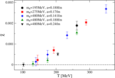
Figure 3: Susceptibility (SI units) as a function of $T$, for different values of $m_{\pi}$ and $a$.

Discussion – Fig. 3 shows that $\tilde{\chi}$ is compatible with zero, within errors, in the confined phase, while it rises roughly linearly with $T$ in the deconfined one. The drastic increase of $\tilde{\chi}$, which is naturally associable to quark liberation, implies a proportional increase of the $B$-dependent (quadratic) contribution to the pressure. Such results are confirmed by a recent approach based on a Taylor expansion in $B$ levkova .

At $m_{\pi}\simeq 480$ MeV, we performed a continuum extrapolation according to: $\tilde{\chi}=A\,(T-\tilde{T})+A^{\prime}\,a^{2}$, which effectively describes all data with $T>170$ MeV ($\chi^{2}/{\rm d.o.f}=2.5/3$), with coefficients $A=1.37(12)\times 10^{-5}$ MeV^-1, $A^{\prime}=-3.80(15)\times 10^{-4}$ GeV² and $\tilde{T}=126(16)$ MeV (multiplication of $A$ and $A^{\prime}$ by 10.9 provides the conversion to $\hat{\chi}$). When $m_{\pi}$ decreases, a modest increase of $\tilde{\chi}$ is observed; one might expect a further slight increase after continuum extrapolation also in this case.

The computation proposed and first performed in this study surely claims for an extension to the physical case. Our results do not suggest drastic changes when decreasing $m_{\pi}$. The inclusion of the strange quark, instead, may increase $\tilde{\chi}$ by about 20%. Indeed, separating the contributions to $\tilde{\chi}$ from $u$ and $d$ quarks, see Eq. (9), one obtains $\tilde{\chi}_{u}\sim 4\,\tilde{\chi}_{d}$, as expected naively on a charge counting basis (see the Appendix for details), and one may expect $\tilde{\chi}_{s}\sim\tilde{\chi}_{d}$.

Future studies should also clarify the behavior of $\tilde{\chi}$ around $T_{c}$ and its relation to confinement/deconfinement: while present results are compatible with zero in the confined phase, improved determinations could better fix the magnitude and sign of $\tilde{\chi}$ below $T_{c}$. An extension to the case of chromomagnetic fields may be interesting as well bari .

Finally, we notice, following Ref. fraga , that the strong paramagnetic behavior, rising with $T$, in the deconfined phase, and the fact that finite $a$ effects tend to diminish it, may explain the lowering of the pseudocritical temperature with $B$ reg0 , and why a different behavior was observed on coarse lattices demusa ; ilgen .

Acknowledgements: We thank E. D’Emilio, E. Fraga and S. Mukherjee for useful discussions. Numerical computations have been performed on computer facilities provided by INFN, in particular on two GPU farms in Pisa and Genoa and on the QUONG GPU cluster in Rome.

Appendix A APPENDIX

In the following we will discuss a few additional results from our simulations, in order to better elucidate some details of our procedure and to check for possible systematic effects.

The first question one could ask regards the stability of the results against a change of the integration procedure, adopted to exploit Eq. (4). To that purpose, we report in Table 2 the results of the integration over one given quantum of field (reference parameters are the same as for Fig. 1), obtained by varying the order of the spline interpolation used by the integrator and/or the number of points over which $M$ is evaluated. It turns out that the integration is extremely stable, with variations well below statistical fluctuations.

$s$	$16$ points	$32$ points
1	0.000596(16)	0.000594(12)
2	0.000594(17)	0.000593(12)
3	0.000592(17)	0.000594(12)
4	0.000592(17)	0.000594(13)

Table 2: Result of the integration of $M$ between $b=3$ and $b=4$ on a $16^{3}\times 4$ lattice (with $m_{\pi}\approx 480$ MeV and $a\approx 0.188$ fm) using different methods: $s$ is the degree of the spline interpolation and the integral is computed starting from meshes of $16$ or $32$ equally spaced points.

A different issue regards the stability of the result against a variation of the free energy interpolation. The simplest, alternative interpolation, consists in allowing for two (or more) different Dirac strings at the same time, located in different points. That is achieved by superposing two $U(1)$ fields like that in Eq. (3), but with one of them shifted in one or two coordinates, so as to move the location of the string: in this way one obtains an interpolation between two consecutive, even quanta, however odd quanta are not possible any more. In Fig. 4 we show, as an example, the values of $M$ between $b=2$ and $b=4$ obtained for the standard and for the alternative interpolation described above: in the latter case, the two Dirac strings pierce the $x,y$ plaquettes located at $(n_{x},n_{y})=(L_{x},L_{y})$ and $(L_{x},L_{y}/2)$, respectively. The corresponding cumulative integrals are reported in Fig. 5: they coincide, within errors, for values of $b$ where strings become invisible for both interpolations, proving the stability of the procedure.

As a further, alternative interpolation, we have also tried to modify the standard one by adding a uniform $U(1)$ background which disappears for integer values of $b$. Results are shown in Figs. 4 and 5 as well, for one single quantum and for the case where a phase $\exp(i2\pi b)$ is added to all links along the $y$ direction: they are perfectly compatible with those from the standard interpolation, even if a statistics larger by a factor 10 had to be used, due to the fact that the observable is much noisier in this case.

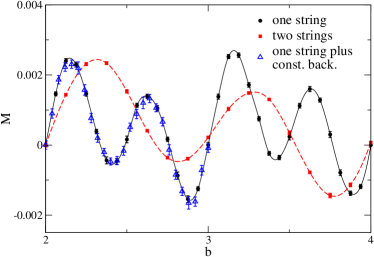
Figure 4: $M$ computed between $b=2$ and $b=4$, and for the same lattice parameters as in Table 2, for three different interpolations of the free energy (see text).

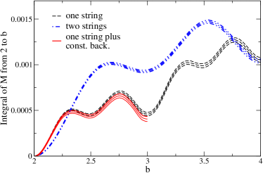
Figure 5: Cumulative integrals of the three functions reported in Fig. 4.

Finally, since the observable $M$ is made up of two different terms, $M_{u}$ and $M_{d}$, coming from each quark determinant (see Eq. (9)), it is interesting to see how the two contributions look like. That is shown in Fig. 6, where the same data shown in Fig. 1 for the $16^{3}\times 4$ lattice have been split accordingly. $M_{u}$ and $M_{d}$ present very similar oscillations, apart from a factor two in the frequency, which can be trivially associated to the electric charge ratio of the two quarks. It is interesting that results can be described by the simplest function which can be devised by requiring that: i) it vanishes at points where the string becomes invisible to the corresponding quark; ii) it has a non-vanishing integral between any consecutive pair of such points; iii) it is an odd function of $b$, as required by the charge conjugation symmetry present at $b=0$. Such function is

$$M^{\rm try}_{q}=A\,\sin\left(2\pi\frac{q}{q_{d}}b\right)+A^{\prime}\,b\,\left(1-\cos\left(2\pi\frac{q}{q_{d}}b\right)\right)\,,$$ (12)

where $q=q_{u}$ or $q=q_{d}$, and fits very well all data in Fig. 6, with $\chi^{2}/{\rm d.o.f.}=0.81$ for the $d$ quark and $\chi^{2}/{\rm d.o.f.}=1.10$ for the $u$ quark. It is easy to check that the integral of such function between 0 and integer values of $b$ equals $A^{\prime}\,b^{2}/2$ (fit values for $A^{\prime}$ are compatible with those from the standard spline integrators), therefore deviations from such simple description are expected as soon as the corrections to the quadratic behavior of $\Delta f$ become visible.

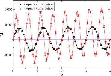
Figure 6: Contributions to $M$ from the $u$ and $d$ quarks, computed on a $16^{3}\times 4$ lattice, with $a\approx 0.188$ fm and $m_{\pi}\approx 480$ MeV. The continuous lines are best fits according to Eq. (12).

Data obtained for $M_{u}$ and $M_{d}$ can be integrated separately for each lattice setup, in this way also the renormalized free energy and the corresponding magnetic susceptibility can be separated into two different contributions, $\tilde{\chi}=\tilde{\chi}_{u}+\tilde{\chi}_{d}$. For the case shown explicitly in Fig. 6, one obtains $\tilde{\chi}_{u}=0.00122(9)$ and $\tilde{\chi}_{d}=0.000315(30)$. Even if one cannot strictly speak of $u$ and $d$ contributions, because of quark loop effects which mix the two terms, it is nice to observe that $\tilde{\chi}_{u}/\tilde{\chi}_{d}=3.9(4)\sim(q_{u}/q_{d})^{2}$, in agreement with a naive charge counting rule. Similar results are obtained for the other values of $T$ and $m_{\pi}$ explored in this study.

References

- (1) R. C. Duncan and C. Thompson, Astrophys. J. 392, L9 (1992).
- (2) V. Skokov, A. Y. Illarionov and V. Toneev, Int. J. Mod. Phys. A 24, 5925 (2009) [arXiv:0907.1396 [nucl-th]].
- (3) V. Voronyuk, V. D. Toneev, W. Cassing, E. L. Bratkovskaya, V. P. Konchakovski and S. A. Voloshin, Phys. Rev. C 83, 054911 (2011) [arXiv:1103.4239 [nucl-t
- (4) A. Bzdak and V. Skokov, Phys. Lett. B 710, 171 (2012) [arXiv:1111.1949 [hep-ph]].
- (5) W. -T. Deng and X. -G. Huang, Phys. Rev. C 85, 044907 (2012) [arXiv:1201.5108 [nucl-th]].
- (6) T. Vachaspati, Phys. Lett. B 265, 258 (1991).
- (7) D. Grasso and H. R. Rubinstein, Phys. Rept. 348, 163 (2001) [astro-ph/0009061].
- (8) D. Kharzeev, K. Landsteiner, A. Schmitt and H. -U. Yee, Lect. Notes Phys. 871, 1 (2013).
- (9) P. V. Buividovich, M. N. Chernodub, E. V. Luschevskaya and M. I. Polikarpov, Nucl. Phys. B 826, 313 (2010) [arXiv:0906.0488 [hep-lat]].
- (10) G. S. Bali, F. Bruckmann, M. Constantinou, M. Costa, G. Endrodi, S. D. Katz, H. Panagopoulos and A. Schafer, Phys. Rev. D 86, 094512 (2012) [arXiv:1209.6015 [hep-lat]].
- (11) G. S. Bali, F. Bruckmann, G. Endrodi, F. Gruber and A. Schaefer, JHEP 1304, 130 (2013) [arXiv:1303.1328 [hep-lat]].
- (12) G. M. Torrie and J. P. Valleau, J. Comp. Phys. 23, 187 (1977).
- (13) G. ’t Hooft, Nucl. Phys. B 153, 141 (1979).
- (14) J. Smit and J. C. Vink, Nucl. Phys. B 286, 485 (1987).
- (15) P. H. Damgaard and U. M. Heller, Nucl. Phys. B 309, 625 (1988).
- (16) M. H. Al-Hashimi and U. J. Wiese, Ann. Phys. 324, 343 (2009) [arXiv:0807.0630 [quant-ph]].
- (17) P. de Forcrand, M. D’Elia and M. Pepe, Phys. Rev. Lett. 86, 1438 (2001) [hep-lat/0007034].
- (18) G. S. Bali, F. Bruckmann, G. Endrodi, Z. Fodor, S. D. Katz, S. Krieg, A. Schafer and K. K. Szabo, JHEP 1202, 044 (2012) [arXiv:1111.4956 [hep-lat]].
- (19) L. D. Landau, E. M. Lifshitz and L. P. Pitaevskii “Electrodynamics of continuous media” Butterworth-Heinemann (2004).
- (20) T. Blum, L. Karkkainen, D. Toussaint and S. A. Gottlieb, Phys. Rev. D 51, 5153 (1995) [hep-lat/9410014].
- (21) M. D’Elia, M. Mariti and F. Negro, Phys. Rev. Lett. 110, 082002 (2013) [arXiv:1209.0722 [hep-lat]].
- (22) C. Bonati, G. Cossu, M. D’Elia and P. Incardona, Comp. Phys. Comm. 183, 853 (2012) [arXiv:1106.5673 [hep-lat]].
- (23) As an example, we report for Platinum and for Liquid Oxygen.
- (24) P. Cea and L. Cosmai, JHEP 0508, 079 (2005); P. Cea, L. Cosmai and M. D’Elia, JHEP 0712, 097 (2007);
- (25) E. S. Fraga, J. Noronha and L. F. Palhares, arXiv:1207.7094 [hep-ph].
- (26) M. D’Elia, S. Mukherjee, F. Sanfilippo, Phys. Rev. D 82, 051501 (2010).
- (27) L. Levkova and C. DeTar, arXiv:1309.1142 [hep-lat].
- (28) E. -M. Ilgenfritz, M. Kalinowski, M. Muller-Preussker, B. Petersson and A. Schreiber, Phys. Rev. D 85, 114504 (2012).