Landau level transitions in doped graphene in a time dependent magnetic field

Abstract

The aim of this work is to describe the Landau levels transitions of Bloch electrons in doped graphene with an arbitrary time dependent magnetic field in the long wavelength approximation. In particular, transitions from the $m$ Landau level to the $m\pm 1$ and $m\pm 2$ Landau levels are studied using time-dependent perturbation theory. Time intervals are computed in which transition probabilities tend to zero at low order in the coupling constant. In particular, Landau level transitions are studied in the case of Bloch electrons travelling in the direction of the applied magnetic force and the results are compared with classical and revival periods of electrical current in graphene. Finally, current probabilities are computed for the $n=0$ and $n=1$ Landau levels showing expected oscillating behavior with modified cyclotron frequency.

1 Introduction

Nowadays, graphene, the most important crystalline forms of carbon, is one of the most significant topics in solid state physics due to the vast application in nano-electronics, opto-electronics, superconductivity and Josephson junctions ([1],[2],[3]). This material is a two-dimensional sheet of carbon atoms forming a honey-comb lattice made of two interpenetrating-bonded triangular sublattices, A and B. The linear band dispersion at the so called Dirac point is a special feature of the graphene band structure which are dictated by the $\pi$ and $\pi^{\prime}$ bands that form conical valleys touching at the high symmetry points of the Brillouin zone [6]. A key point is that the linear dispersion near the symmetry points have striking similarities with those of massless relativistic Dirac fermions or an effective Dirac-Weyl Hamiltonian [4]. This leads to a number of fascinating phenomena such as the half-quantized Hall effect ([7],[8]) and minimum quantum conductivity in the limit of vanishing concentration of charge carriers [1]. Another of the effects that change their form, comparing to the electrons described by Schrödinger equation, are the Landau levels. These are quantized energy levels for electrons in a magnetic field. They still appear also for relativistic electrons, just their dependence on field and quantization parameter is different. In a conventional non-relativistic electron gas, Landau quantization produces equidistant energy levels, which is due to the parabolic dispersion law of free electrons. In graphene, the electrons have relativistic dispersion law, which strongly modifies the Landau quantization of the energy and the position of the levels. In particular, they are not equidistant as in conventional case and the largest energy separation is between the zero and the first Landau level (for multilayer graphene see [9]). This large gap allows one to observe the quantum Hall effect in graphene, even at room temperature [10]. Experimentally, the Landau levels in graphene have been observed by measuring cyclotron resonances of the electrons and holes in infrared spectroscopy experiments [11] and by measuring tunneling current in scanning tunneling spectroscopy experiments [12]. The experimental study of the $n=0$ Landau level has attracted a great deal of attention, and has evolved rapidly, as better quality samples become available, and higher magnetic fields and lower temperatures were studied ([13],[14],[15], [16]), but in particular, Landau level mixing is neglected (see [17], [18]), and this is not as clearly justified because the single particle Landau level gaps in graphene scale as $\sqrt{B}$, which is the same as the interaction strength [19]. In turn, only optical transitions between Landau levels has been calculated. Since in graphene both conduction and valence bands have the same symmetry, the optical transition selection rule has the same form for both intraband and interband transition, and is given by the relation $n=m\pm 1$ (see [20] and [21]).

In the other side, it is commonly accepted that graphene has very few lattice defects. Doped graphene shows remarkable high field-effect mobilities, even at room temperatures ([22],[23]). Also it is possible the appearance of negative conductivity in graphene with impurities in magnetic fields (see [24] and [25]).

In turn, Landau level shift in graphene monolayer subjected to a quantizing perpendicular magnetic field under the influence of short-range $\delta$-potential impurities has been studied using Green function method [26]. However, Landau level transitions in graphene with impurities placed in a time-dependent magnetic field has not been theoretically studied, therefore in this work we address this problem using time-dependent perturbation theory, where the free Hamiltonian is defined on eq.(2) of [25], and the interacting Hamiltonian is defined in eq.(6) of this work. In particular, the case in which at $t=0$ the quantum state is in the $m$ Landau level and the possible transition to the $m\pm 1$ and $m\pm 2$ Landau level is studied and its relation to revivals and zitterbewegung effect is analized (see [27]).

The work is organized as follows:

In Section 2, the free Hamiltonian and the interacting Hamiltonian are introduced and the time-dependent perturbation theory is applied.

In Section 3, transition probabilities from $m$ to $m\pm 1$ and $m\pm 2$ Landau levels are computed and time intervals in which probabilities goes to zero are obtained in terms of the Hamiltonian parameters.

In Section 4, transitions from the $n=0~{}$Landau level to the $n=1\$Landau level are computed and analyzed. Current probability is obtained showing the expected circular motion with cyclotron frequency.

In section 5, the conclusions are presented.

In Appendix A and C the conservation of probability and current density is computed and in Appendix B some useful formulas are introduced.

2 Graphene Hamiltonian with impurity placed in a time-dependent magnetic field

The Hamiltonian of graphene near the Dirac point $K$ in the long wavelength approximation reads

$$H=v_{f}(\sigma_{x}p_{x}+\sigma_{y}p_{y})$$ (1)

where $v_{f}$ is the Fermi velocity that is defined as $v_{f}=\frac{\sqrt{3}ta}{2\hbar}$, where $t\approx 3eV$ and $a=0.246nm$ (see [28]), $\sigma_{x}$ and $\sigma_{y}$ are the Pauli matrices and $p_{x}$ and $p_{y}$ are the momentum of the Bloch electrons in the graphene plane monolayer). This Hamiltonian acts on the electron wavefunctions localized on sublattice $A$ and $B$ respectively. Using the tight binding approximation, is not difficult to show that if we place an impurity near the atom of the sublattice $A$ and $B$, the corresponding Hamiltonian can be written as (see [25])

$$H=\left(\begin{array}[]{cccc}0&v_{f}(p_{x}-ip_{y})&U&0\\ v_{f}(p_{x}+ip_{y})&0&0&U\\ U&0&\varepsilon&0\\ 0&U&0&\varepsilon\end{array}\right)$$ (2)

where $U$ is the hybridization potential which reflects the overlap energy between the $p_{z}$ orbital of the electron in carbon atom and the arbitrary orbital of the impurity atom, and $\varepsilon$ is the energy of the absorbed impurity atom with respect to the Fermi level (these values can be evaluated experimentally (see [29])). The electron wavefunctions will be a four component vector $\psi=\left(\rho_{A},\rho_{B},\upsilon_{A},\upsilon_{B}\right)$, where the first two components correspond to $K$ Dirac point and the remaining two components correspond to the wave function of electrons localized on the impurity.

If we place the graphene perpendicular to a time dependent magnetic field, the momentum of the Bloch electrons will be changed as $\overrightarrow{p}\rightarrow\overrightarrow{p}-e\overrightarrow{A}$ where $\overrightarrow{A}$ is the potential vector and $e$ is the electron charge. In particular, we can choose the following gauge $\overrightarrow{A}=(-B(t)y,0,0).$ In this case, the Hamiltonian reads

$$H=\left(\begin{array}[]{cccc}0&v_{f}(p_{x}+eB(t)y-ip_{y})&U&0\\ v_{f}(p_{x}+eB(t)y+ip_{y})&0&0&U\\ U&0&\varepsilon&0\\ 0&U&0&\varepsilon\end{array}\right)$$ (3)

In the following, we will assume that the magnetic field will have the following time dependence

$$B(t)=B_{0}+\lambda B_{I}(t)$$ (4)

where $\lambda\leq 1$ is a dimensionless coupling constant and where $B_{I}(t)$ is an arbitrary time-dependent magnetic field. Introducing eq.(4) on eq.(3) we can separate the Hamiltonian in two parts $H=H_{0}+\lambda V(t)$, where

$$H_{0}=\left(\begin{array}[]{cccc}0&v_{f}(p_{x}+eB_{0}y-ip_{y})&U&0\\ v_{f}(p_{x}+eB_{0}y+ip_{y})&0&0&U\\ U&0&\varepsilon&0\\ 0&U&0&\varepsilon\end{array}\right)$$ (5)

and

$$V(t)=\left(\begin{array}[]{cccc}0&v_{f}eB_{I}(t)y&0&0\\ v_{f}eB_{I}(t)y&0&0&0\\ 0&0&0&0\\ 0&0&0&0\end{array}\right)$$ (6)

The wave function can be written as $\psi=e^{-ik_{x}x}\left(\psi_{A},\psi_{B},\xi_{A},\xi_{B}\right)$ where $k_{x}\sim 1/a$ in order to describe the low-energy excitations, i.e. electronic excitations where the charateristic energy may concentrate on excitations at the Fermi level and $\psi_{A}(\psi_{B})$ and $\xi_{A}(\xi_{B})$ are functions that depend on $y$. If we make the following coordinate transformation

$$\overline{y}=-\hbar k_{x}+eB_{0}y$$ (7)

and then we make a scale transformation on $\overline{y}$ as $\overline{y}=\overline{\overline{y}}\,\sqrt{e\hbar B_{0}}$, then the free Hamiltonian reads

$$H_{0}=\left(\begin{array}[]{cccc}0&\gamma a^{{\dagger}}&U&0\\ \gamma a&0&0&U\\ U&0&\varepsilon&0\\ 0&U&0&\varepsilon\end{array}\right)$$ (8)

where $\gamma=v_{f}\sqrt{2e\hbar B_{0}}$ and $a$ and $a^{{\dagger}}$ are creation and annihilation operators

$$a=\frac{1}{\sqrt{2}}\left(\overline{\overline{y}}+\frac{d}{d\overline{\overline{y}}}\right)\text{ \ \ \ \ \ \ \ \ \ \ \ }a^{{\dagger}}=\frac{1}{\sqrt{2}}\left(\overline{y}-\frac{d}{d\overline{\overline{y}}}\right)$$ (9)

that satisfy the commutation relations $\left[a,a^{{\dagger}}\right]=I$.

The eigenvalues and eigenstates for the Hamiltonian of eq.(8) then reads

$$E_{n}^{(i,j)}=\frac{1}{2}\left(\varepsilon+(-1)^{i}\gamma\sqrt{n}+(-1)^{j}\sqrt{(\gamma\sqrt{n}+(-1)^{i+1}\varepsilon)^{2}+4U^{2}}\right)$$ (10)

where $i=1$, $j=1$ gives the energy levels of holes (valence band) in the impurity atom, $i=1$, $j=2$ the energy levels of electrons (conduction band) in the impurity atom, $i=2$, $j=1$ the energy levels of holes in the carbon atom and $i=2$, $j=2$ the energy levels of electrons in carbon atom. The impurities introduce a band gap $\Delta E=\sqrt{\varepsilon^{2}+4U^{2}}$, which implies that doped graphene becomes a semiconductor. The associated eigenvectors reads

$$\varphi_{n}^{(i,j)}(\overline{\overline{y}})=\left(\begin{array}[]{c}\alpha_{n}^{(i,j)}\phi_{n}(\overline{\overline{y}})\\ (-1)^{i}\alpha_{n}^{(i,j)}\phi_{n-1}(\overline{\overline{y}})\\ (-1)^{i}\phi_{n}(\overline{\overline{y}})\\ \phi_{n-1}(\overline{\overline{y}})\end{array}\right)$$ (11)

where $\phi_{n}$ is the eigenstate of the quantum harmonic oscillator and

$$\alpha_{n}^{(i,j)}=\frac{1}{2U}\left(\gamma\sqrt{n}+(-1)^{i+1}\varepsilon+(-1)^{i+j}\sqrt{(\gamma\sqrt{n}+(-1)^{i+1}\varepsilon)^{2}+4U^{2}}\right)$$ (12)

With the knowledge of the eigenfunctions of $H_{0}$, time-dependent perturbation theory can be applied, where the perturbation is $\lambda V(t)$. In particular it will be assumed that from $t=-\infty$ to $t=0$ the magnetic field is $B(t)=B_{0}$ and from $t=0$ to $t=+\infty$, $B(t)=B_{0}+\lambda B_{I}(t)$. In this sense, the basis of eigenvectors of $H_{0}$ can be written as the direct sum of four subspaces, each for energy band. Each subspace is expand by a infinite basis defined by the harmonic oscillator eigenfunctions. In this work we will study the possible transitions within an energy band, which in algebraic terms implies that we will expand the wave function of the full Hamiltonian in terms of the basis of one subspace of the direct sum.

2.1 Time dependent perturbation theory

As we said in the previous section we will study the possible transitions of the different Landau levels in the conduction band of electrons in carbon atoms, then $i=2$ and $j=2$.

The wave function of the Bloch electrons in graphene near the impurity in the long wave-length approximation can be written as

$$\psi(x,\overline{\overline{y}},t)=\sum\limits_{n=0}^{+\infty}c_{n}(t)e^{-ik_{x}x}\varphi_{n}(\overline{\overline{y}})e^{-\frac{i}{\hbar}E_{n}t}$$ (13)

where the $c_{n}(t)$ coefficients represent the probability amplitude of the perturbed quantum system in the $n$-state (see Appendix A). The matrix equation for the coefficients reads

$$i\hbar\frac{dc_{m}}{dt}=\lambda\sum\limits_{n=0}^{+\infty}\left(\int\varphi_{m}^{\ast}(\overline{\overline{y}})V(t)\varphi_{n}(\overline{\overline{y}})d\overline{\overline{y}}dx\right)e^{-i\omega_{(n,m)}t}c_{n}(t)$$ (14)

where

$$\omega_{(n,m)}=\frac{1}{\hbar}(E_{n}-E_{m})=\frac{1}{2\hbar}\left(\gamma\left(\sqrt{n}-\sqrt{m}\right)+\sqrt{(\gamma\sqrt{n}-\varepsilon)^{2}+4U^{2}}-\sqrt{(\gamma\sqrt{m}-\varepsilon)^{2}+4U^{2}}\right)$$ (15)

are the spectral frequencies. Applying $V(t)$ on $\varphi_{n}(\overline{\overline{y}})$ and computing the scalar product with $\varphi_{m}^{\ast}(\overline{\overline{y}})$ we obtain

$$\int\varphi_{m}^{\ast}(\overline{\overline{y}})V(t)\varphi_{n}(\overline{\overline{y}})d\overline{\overline{y}}dx=-\frac{\alpha_{n}\alpha_{m}\eta(t)}{\sqrt{(\alpha_{n}^{2}+1)(\alpha_{m}^{2}+1)}}[\beta\left(\delta_{m,n-1}+\delta_{m-1,n}\right)$$ (16)

$$+\frac{\xi\eta(t)}{\sqrt{2}}\left(\sqrt{n-1}\delta_{m,n-2}+\sqrt{n}\delta_{mn}+\sqrt{n}\delta_{m-1,n-1}+\sqrt{n+1}\delta_{m-1,n+1}\right)]$$

where $\beta=\,v_{f}\sqrt{e\hbar B_{0}}=\sqrt{2}\gamma$, $\xi=v_{f}\hbar k_{x}$, $\eta(t)=\frac{B_{I}(t)}{B_{0}}$ and where it has been used that $v_{f}eB_{I}(t)y=\eta(t)(\beta\overline{\overline{y}}+\xi)$ and $\overline{\overline{y}}=\frac{1}{\sqrt{2}}(a+a^{{\dagger}})$. Introducing last equation on eq.(14) we obtain a coupled system of differential equations for the $c_{m}~{}$coefficients

$$i\hbar\frac{dc_{m}}{dt}=-\lambda(\frac{\alpha_{m}^{2}\eta(t)}{\alpha_{m}^{2}+1}\xi\sqrt{2m}c_{m}(t)+\frac{\alpha_{m+1}\alpha_{m}\eta(t)}{\sqrt{(\alpha_{m+1}^{2}+1)(\alpha_{m}^{2}+1)}}\beta e^{-i\omega_{(m+1,m)}t}c_{m+1}(t)$$ (17)

$$+\frac{\alpha_{m-1}\alpha_{m}\eta(t)}{\sqrt{(\alpha_{m-1}^{2}+1)(\alpha_{m}^{2}+1)}}\beta e^{-i\omega_{(m-1,m)}t}c_{m-1}(t)+\frac{\alpha_{m+2}\alpha_{m}\eta(t)}{\sqrt{(\alpha_{m+2}^{2}+1)(\alpha_{m}^{2}+1)}}\xi\sqrt{\frac{m+1}{2}}e^{-i\omega_{(m+2,m)}t}c_{m+2}(t)$$

$$+\frac{\alpha_{m-2}\alpha_{m}\eta(t)}{\sqrt{(\alpha_{m-2}^{2}+1)(\alpha_{m}^{2}+1)}}\xi\sqrt{\frac{m-1}{2}}e^{-i\omega_{(m-2,m)}t}c_{m-2}(t))$$

Last equation indicates that the contribution to the $m$-state comes from the $m-2$, $m-1$, $m$, $m+1$ and $m+2$ states.

The perturbation approximation is introduced by expanding the coefficients in powers of $\lambda$ (see eq.(12.48) of [30], page 350), then at order $\lambda^{0}$ and order $\lambda^{k}$ we obtain the following relations among the coefficients

$$\frac{dc_{m}^{(0)}}{dt}=0$$ (18)

and

$$i\hbar\frac{dc_{m}^{(k)}}{dt}=-\frac{\alpha_{m}^{2}}{\alpha_{m}^{2}+1}\xi\sqrt{2m}\eta(t)c_{m}^{(k-1)}(t)-\frac{\alpha_{m+1}\alpha_{m}}{\sqrt{(\alpha_{m+1}^{2}+1)(\alpha_{m}^{2}+1)}}\beta e^{-i\omega_{(m+1,m)}t}\eta(t)c_{m+1}^{(k-1)}(t)$$ (19)

$$-\frac{\alpha_{m-1}\alpha_{m}}{\sqrt{(\alpha_{m-1}^{2}+1)(\alpha_{m}^{2}+1)}}\beta e^{-i\omega_{(m-1,m)}t}\eta(t)c_{m-1}^{(k-1)}(t)$$

$$-\frac{\alpha_{m+2}\alpha_{m}}{\sqrt{(\alpha_{m+2}^{2}+1)(\alpha_{m}^{2}+1)}}\xi\sqrt{\frac{m+1}{2}}e^{-i\omega_{(m+2,m)}t}\eta(t)c_{m+2}^{(k-1)}(t)$$

$$-\frac{\alpha_{m-2}\alpha_{m}}{\sqrt{(\alpha_{m-2}^{2}+1)(\alpha_{m}^{2}+1)}}\xi\sqrt{\frac{m-1}{2}}e^{-i\omega_{(m-2,m)}t}\eta(t)c_{m-2}^{(k-1)}(t)$$

where the superscript in $c_{m}^{(k)}$ indicates the order of $\lambda$ and the subscript indicates the Landau level. In the following section we will study the possible transitions from the $m$ state to the $m\pm 1$ and $m\pm 2$ states under different conditions up to second order in the perturbation expansion.

3 Transition probabilities from $m$ to $m\pm 1$ and $m\pm 2$ Landau levels

Using eq.(19) and assuming that at $t=0$ the quantum state is in the $m$ state, that is $c_{m}^{(0)}=1$ and $c_{k}^{(0)}=0$ for $k\neq m$, we obtain for $c_{m}^{(1)}(t)$, $c_{m-1}^{(1)}(t)$, $c_{m+1}^{(1)}(t)$, $c_{m-2}^{(1)}(t)$ and $c_{m+2}^{(1)}(t)$ the following equations

$$c_{m}^{(1)}=-\frac{\alpha_{m}^{2}}{i\hbar(\alpha_{m}^{2}+1)}\xi\sqrt{2m}f_{(0,0)}(t)$$ (20)

$$c_{m+1}^{(1)}=-\frac{\alpha_{m}\alpha_{m+1}}{i\hbar\sqrt{(\alpha_{m}^{2}+1)(\alpha_{m+1}^{2}+1)}}\beta f_{(m,m+1)}(t)$$ (21)

$$c_{m-1}^{(1)}=-\frac{\alpha_{m}\alpha_{m-1}}{i\hbar\sqrt{(\alpha_{m}^{2}+1)(\alpha_{m-1}^{2}+1)}}\beta f_{(m,m-1)}(t)$$ (22)

$$c_{m+2}^{(1)}=-\frac{\alpha_{m}\alpha_{m+2}}{i\hbar\sqrt{(\alpha_{m}^{2}+1)(\alpha_{m+2}^{2}+1)}}\xi\sqrt{\frac{m+1}{2}}f_{(m,m+2)}(t)$$ (23)

$$c_{m-2}^{(1)}=-\frac{\alpha_{m}\alpha_{m-2}}{i\hbar\sqrt{(\alpha_{m}^{2}+1)(\alpha_{m-2}^{2}+1)}}\xi\sqrt{\frac{m-1}{2}}f_{(m,m-2)}(t)$$ (24)

where

$$f_{(n,m)}(t)=\int_{0}^{t}\eta(t^{\prime})e^{-i\omega_{(n,m)}t^{\prime}}dt^{\prime}$$ (25)

and $c_{k}^{(1)}=0$ for $k<m-2$ and $k>m+2$. From eq.(23) and eq.(24), it can be noted that the $c_{m\pm 2}^{(2)}$ coefficients depend on $\xi$, which is a function of the wave vector $k_{x}$. Because we will study the transition probabilities up to order $\lambda^{2}$, we must compute the $c_{m}^{(2)}$ coefficient which reads

$$c_{m}^{(2)}=-\frac{\alpha_{m}^{2}}{\hbar^{2}(\alpha_{m}^{2}+1)}[\xi^{2}\left(\frac{2m\alpha_{m}^{2}}{(\alpha_{m}^{2}+1)}F_{(0,0)}^{(0,0)}(t)+\frac{\alpha_{m+2}^{2}(m+1)}{2(\alpha_{m+2}^{2}+1)}F_{(m,m+2)}^{(m+2,m)}(t)+\frac{\alpha_{m-2}^{2}(m-1)}{2(\alpha_{m-2}^{2}+1)}F_{(m,m-2)}^{(m-2,m)}(t)\right)$$ (26)

$$+\beta^{2}\left(\frac{\alpha_{m+1}^{2}}{(\alpha_{m+1}^{2}+1)}F_{(m,m+1)}^{(m+1,m)}(t)+\frac{\alpha_{m-1}^{2}}{(\alpha_{m-1}^{2}+1)}F_{(m,m-1)}^{(m-1,m)}(t)\right)]$$

where

$$F_{(n,m)}^{(n^{\prime},m^{\prime})}(t)=\int_{0}^{t}e^{-i\omega_{(n^{\prime},m^{\prime})}t^{\prime}}\eta(t^{\prime})f_{(n,m)}(t^{\prime})dt^{\prime}$$ (27)

Using the Taylor expansion of eq.(25) and eq.(27) in Appendix B, the probabilities up to order $\lambda^{2}$ and order $t^{2}$ reads

$$P_{m}(t)=1-\frac{\lambda^{2}\alpha_{m}^{2}\eta_{0}^{2}t^{2}}{\hbar^{2}(\alpha_{m}^{2}+1)}\times$$ (28)

$$\left[\xi^{2}\left(\frac{2m\alpha_{m}^{2}}{\alpha_{m}^{2}+1}+\frac{\alpha_{m+2}^{2}(m+1)}{2(\alpha_{m+2}^{2}+1)}+\frac{\alpha_{m-2}^{2}(m-1)}{2(\alpha_{m-2}^{2}+1)}\right)+\beta^{2}\left(\frac{\alpha_{m+1}^{2}}{(\alpha_{m+1}^{2}+1)}+\frac{\alpha_{m-1}^{2}}{(\alpha_{m-1}^{2}+1)}\right)\right]+O(\lambda^{3},t^{3})$$

for $P_{m\pm 1}(t)$ we obtain

$$P_{m+1}(t)=\lambda^{2}\frac{\alpha_{m}^{2}\alpha_{m+1}^{2}\beta^{2}}{\hbar^{2}(\alpha_{m}^{2}+1)(\alpha_{m+1}^{2}+1)}\eta_{0}^{2}t^{2}+O(\lambda^{3},t^{3})$$ (29)

$$P_{m-1}(t)=\lambda^{2}\frac{\alpha_{m}^{2}\alpha_{m-1}^{2}\beta^{2}}{\hbar^{2}(\alpha_{m}^{2}+1)(\alpha_{m-1}^{2}+1)}\eta_{0}^{2}t^{2}+O(\lambda^{3},t^{3})$$ (30)

and for $P_{m\pm 2}(t)$ we obtain

$$P_{m+2}(t)=\lambda^{2}\frac{\alpha_{m}^{2}\alpha_{m+2}^{2}\xi^{2}(m+1)}{2\hbar^{2}(\alpha_{m}^{2}+1)(\alpha_{m+2}^{2}+1)}\eta_{0}^{2}t^{2}+O(\lambda^{3},t^{3})$$ (31)

$$P_{m-2}(t)=\lambda^{2}\frac{\alpha_{m}^{2}\alpha_{m-2}^{2}\xi^{2}(m-1)}{2\hbar^{2}(\alpha_{m}^{2}+1)(\alpha_{m-2}^{2}+1)}\eta_{0}^{2}t^{2}+O(\lambda^{3},t^{3})$$ (32)

where $\eta_{0}=B_{I}(0)/B_{0}$ is a dimensionless constant. From last equation is not difficult to see that $P_{m}(t)$ contains the coefficients that appears in $P_{m+1}(t)$, $P_{m-1}(t)$, $P_{m+2}(t)$ and $P_{m-2}(t)$, that is

$$P_{m}(t)=1-\lambda^{2}\frac{2m\alpha_{m}^{4}\eta_{0}^{2}t^{2}\xi^{2}}{\hbar^{2}(\alpha_{m}^{2}+1)^{2}}-P_{m+2}(t)-P_{m-2}(t)-P_{m+1}(t)-P_{m-1}(t)$$ (33)

The second term of r.h.s. of last equation, which is the contribution at first order in $\lambda$ of the probability amplitude of the $m$ Landau level, prevents that Bloch electrons behave as a five-level system in the following time interval

$$\Delta t=\frac{\hbar\sqrt{\alpha_{m}^{2}+1}}{\lambda\alpha_{m}\eta_{0}\sqrt{\xi^{2}\left(\frac{2m\alpha_{m}^{2}}{\alpha_{m}^{2}+1}+\frac{\alpha_{m+2}^{2}(m+1)}{2(\alpha_{m+2}^{2}+1)}+\frac{\alpha_{m-2}^{2}(m-1)}{2(\alpha_{m-2}^{2}+1)}\right)+\beta^{2}\left(\frac{\alpha_{m+1}^{2}}{(\alpha_{m+1}^{2}+1)}+\frac{\alpha_{m}^{2}}{(\alpha_{m-1}^{2}+1)}\right)}}$$ (34)

which is defined as the time at which $P_{m}(t)$ is zero. The limits $m\rightarrow 0$ reads

$$\underset{m\rightarrow 0}{\lim}\Delta t=\frac{2\hbar\sqrt{4u^{2}+\epsilon(\epsilon+\sqrt{4u^{2}+\epsilon^{2}})}}{(\epsilon+\sqrt{4u^{2}+\epsilon^{2}})\eta\beta\sqrt{\frac{(\epsilon+\sqrt{4u^{2}+\epsilon^{2}})^{2}}{4u^{2}+\epsilon(\epsilon+\sqrt{4u^{2}+\epsilon^{2}})}+\frac{2(\sqrt{z}\beta+\sqrt{2}\epsilon+\sqrt{8u^{2}+z\beta^{2}+2\sqrt{z}\beta\epsilon+2\epsilon^{2}})^{2}}{8u^{2}+(\sqrt{z}\beta+\sqrt{2}\epsilon+\sqrt{8u^{2}+z\beta^{2}+2\sqrt{z}\beta\epsilon+2\epsilon^{2}})^{2}}}}$$ (35)

Figure 1: $\Delta t$ as a function of $m$ for $z=3$(violet), $z=4$ (blue), $z=5$ (red) and $z=6$ (green).

In particular, using typical values, for example, $U=-1.43eV$, $\varepsilon=-3eV$, $\xi=9/2eV$, $\gamma=\frac{\beta}{\sqrt{2}}=0.043\sqrt{\frac{z}{2}}eV$, where $z$ is a dimensioneless parameter that quantifies the magnetic field strength $B_{0}$ (we use $z=5$) and $B_{I}(0)=5T$, so $\eta_{0}=1$, the limit of $\Delta t$ when $m\rightarrow 0$ is about $\Delta t\sim 1.55\times 10^{-15}s$, which is in the order of the optical spectrum for electromagnetic waves. This value can be compared with the classical period and the revival time of electron current in graphene under a constant magnetic field (see [27]), which do not depends on the presence or ausence of impurities. Both values $T_{CL}=\frac{4\pi}{v_{f}}\sqrt{\frac{m\hbar}{2eB_{0}}}$ and $T_{R}=\frac{16\pi m^{3/2}}{v_{f}}\sqrt{\frac{\hbar}{2eB_{0}}}$ are of the order of $10^{-12}s$ for $B_{0}=10T$ and where $m$ is the Landau level index. The main difference between the values found in this section and the approach of [27] is that in the latter a superposition of two wave packets, one from the conduction band and the other from the valence band, are used. In turn, the zitterbewegung effect, which is related with the interference between positive and negative frequency components of wave packets superposition of both positive and negative energies shows up with a period $T_{ZB}=\pi\sqrt{\frac{\hbar}{m2eB_{0}}}$. In [27] values of $T_{ZB}$ are of the order of $10^{-15}s$ which coincide with the values computed in eq.(35)). The similar values for $\Delta t$ and $T_{ZB}$ implies that we must consider the contribution of the valence band to the wave function superposition of eq.(13). In that case, $V(t)$ will not introduce coupling effects between the conduction and valence band transitions amplitudes and a similar Landau level transitions will appear in the valence band. In the next section we will show how the $T_{ZB}$ can be related with $\Delta t$ in a more direct way. In figure 1, $\Delta t$ is plotted against $m$ for various values of $z$. The figure shows relevant initial Landau levels where $\Delta t$ reaches a minimum, which is the shortest time scale that characterizes the spread of the $m$ Landau level energy to the $m\pm 1$ and $m\pm 2$ Landau level energies as a function of $m$. Using that $\Delta E\sim\left|E_{m_{0}+1}+E_{m_{0}-1}+E_{m_{0}+2}+E_{m_{0}-2}-E_{m_{0}}\right|$, where $m_{0}$ is the Landau level at which $\Delta t$ reaches the minimum, the uncertainty principle saturate at the time interval $\Delta T(m_{0})\sim\frac{\hbar}{2\Delta E(m_{0})}$ which is smaller than $\Delta t$; using the values above $\Delta T(m_{0})/\Delta t(m_{0})\sim 10^{-3}$. This implies that we cannot obtain a coherent state in the time interval in which the $m$, $m\pm 1$ and $m\pm 2$ Landau levels get mixed.

The ratio between the considered Landau levels reads

$$\frac{P_{m-1}(t)}{P_{m+1}(t)}=\frac{\alpha_{m-1}^{2}(\alpha_{m+1}^{2}+1)}{\alpha_{m+1}^{2}(\alpha_{m-1}^{2}+1)}$$ (36)

and

$$\frac{P_{m-2}(t)}{P_{m+2}(t)}=\frac{\alpha_{m-2}^{2}(m-1)(\alpha_{m+2}^{2}+1)}{\alpha_{m+2}^{2}(m+1)(\alpha_{m-2}^{2}+1)}$$ (37)

In figure 1, both ratio between probabilities are plotted using the values used above.

Figure 2: $\frac{P_{m-1}(t)}{P_{m+1}(t)}$ (blue) and $\frac{P_{m-2}(t)}{P_{m+2}(t)}$ (red) as function of Landau level index $m$.

Both ratio probabilities have the same limit $\underset{m\rightarrow\infty}{\lim}\frac{P_{m-1}(t)}{P_{m+1}(t)}=\underset{m\rightarrow\infty}{\lim}\frac{P_{m-2}(t)}{P_{m+2}(t)}=1$ and from figure 1, $P_{m-1}(t)<P_{m+1}(t)$ and $P_{m-2}(t)<P_{m+2}(t)$, which implies that the initial probability flows from the $m$ state to the $m+1$ and $m+2$ states faster than to the $m-1$ and $m-2$ states.

3.1 Bloch electrons travelling in the $y$ direction ($k_{x}=0$)   

In this case, $\xi=0$, then the $P_{m\pm 2}=0$ at order $\lambda^{2}$ because $c_{m\pm 2}^{(1)}(t)=0$ (see eq.(23) and eq.(24)), $P_{m\pm 1}$ remains the same and $P_{m}(t)$ reads

$$P_{m}(t)=1-\frac{\lambda^{2}\alpha_{m}^{2}\eta_{0}^{2}t^{2}\beta^{2}}{\hbar^{2}(\alpha_{m}^{2}+1)}\left(\frac{\alpha_{m+1}^{2}}{(\alpha_{m+1}^{2}+1)}+\frac{\alpha_{m-1}^{2}}{(\alpha_{m-1}^{2}+1)}\right)$$ (38)

From last equation and eq.(29) and eq.(30) we obtain the following relation between probabilities

$$P_{m}(t)+P_{m+1}(t)+P_{m-1}(t)=1$$ (39)

in the time interval

$$\Delta t=\frac{\hbar}{\lambda\alpha_{m}\beta\eta_{0}}\sqrt{\frac{(\alpha_{m}^{2}+1)(\alpha_{m+1}^{2}+1)(\alpha_{m-1}^{2}+1)}{\alpha_{m+1}^{2}(\alpha_{m-1}^{2}+1)+\alpha_{m-1}^{2}(\alpha_{m+1}^{2}+1)}}$$ (40)

In the case $k_{x}=0$, Bloch electrons behave as a three-level system in the time interval defined in last equation, where the initial probability flows from the $m$ state to the $m\pm 1$ states. The limit for $m\rightarrow\infty$ of $\Delta t$ reads

$$\underset{m\rightarrow\infty}{\lim}\Delta t=\frac{\hbar}{\sqrt{2}\beta\eta_{0}}$$ (41)

Using typical values, this limit is about $\Delta t\sim 10^{-13}\frac{B_{0}}{B_{I}(0)}s$ which is again in the order of optical spectrum for $\frac{B_{0}}{B_{I}(0)}\sim 1$. This time can be larger in those cases in which $B_{0}$ is bigger than $B_{I}(0)$. In this case, $\Delta t$ do not reaches a minimum for same $m$ value. The ratio between $\Delta t$ of eq.(41) and $T_{CL}$ and $T_{R}$ is $T_{CL}/\Delta t=4\pi\sqrt{m}\eta_{0}$ and $T_{R}/T_{CL}=16\pi m^{3/2}\eta_{0}$, which coincide when $m=(4\pi\eta_{0})^{-2}$ and $m=(16\pi\eta_{0})^{-2/3}$. In figure 2 the probability $P_{m}(t)$ and $P_{m+1}$ is shown at order $\lambda^{2}$ for several values of $m$. The probability $P_{m-1}$ can be deduced from eq.(39).

Figure 3: $P_{m}(t)$ and $P_{m+1}$ probabilities as a function of time (for larger $m$, $P_{m}(t)$ goes to zero more faster).

A final remark about the probability is the $m\rightarrow\infty$ limit in eq.(17) in the case $\xi=0$

$$\underset{m\rightarrow\infty}{\lim}\frac{\alpha_{m+1}\alpha_{m}\beta}{i\hbar\sqrt{(\alpha_{m+1}^{2}+1(\alpha_{m}^{2}+1))}}\eta(t)e^{-i\omega_{(m+1,m)}t}=\frac{\beta}{i\hbar}\eta(t)$$ (42)

and

$$\underset{m\rightarrow\infty}{\lim}\frac{\alpha_{m-1}\alpha_{m}\beta}{i\hbar\sqrt{(\alpha_{m-1}^{2}+1(\alpha_{m}^{2}+1))}}\eta(t)e^{-i\omega_{(m-1,m)}t}=\frac{\beta}{i\hbar}\eta(t)$$ (43)

In turn if we consider

$$\underset{m\rightarrow\infty}{\lim}c_{m+1}\sim\underset{m\rightarrow\infty}{\lim}c_{m-1}\sim c_{\infty}$$ (44)

for $m\rightarrow\infty$, eq.(17) reads

$$\frac{dc_{\infty}}{dt}=-\frac{2i\beta}{\hbar}\eta(t)c_{\infty}$$ (45)

which has a trivial solution

$$c_{\infty}(t)=c_{\infty}(t_{0})\exp\left(-\frac{2i\beta}{\hbar B_{0}}\int_{t_{0}}^{t}B_{I}(t^{\prime})dt^{\prime}\right)$$ (46)

A particular case can be given when

$$\int_{t_{0}}^{t}B_{I}(t^{\prime})dt^{\prime}=\mathrm{Re}(g(t))-i\mathrm{Im}(g(t))$$ (47)

Then

$$\left|c_{\infty}(t)\right|^{2}=\left|c_{\infty}(t_{0})\right|^{2}e^{-\frac{4\beta}{\hbar}\mathrm{Im}(g(t))}$$ (48)

which implies that a contribution to the probability is given by the imaginary part of the integral of the time-dependent magnetic field. For example, in an oscillating magnetic field $B_{I}(t)=B_{I}e^{-i\omega t}$, the imaginary part of the integral of the magnetic field reads

$$\mathrm{Im}(g(t))=\frac{B_{I}}{\omega}(-1+\cos\omega t)$$ (49)

then the probability $\left|c_{\infty}(t)\right|^{2}$ is oscillatory

$$\left|c_{\infty}(t)\right|^{2}=\left|c_{\infty}(t_{0})\right|^{2}e^{-\frac{4\beta}{\hbar}\frac{B_{I}}{\omega}(-1+\cos\omega t)}$$ (50)

with a frequency identical to the magnetic field $B_{I}(t)$.

4 Transition from $n=0$ to $n=1$ Landau level

Of particular interest is the case in which the initial state is in the $n=0$ Landau level, that is, $c_{0}^{(0)}=1$ and $k_{x}=0$. The unique probabilities that contribute at order $\lambda^{2}$ comes from the $n=0$ and $n=1$ Landau level

$$P_{0}(t)=1-\frac{\lambda^{2}\alpha_{0}^{2}\alpha_{1}^{2}\beta^{2}\eta_{0}^{2}}{\hbar^{2}(\alpha_{0}^{2}+1)(\alpha_{1}^{2}+1)}t^{2}+O(\lambda^{3},t^{3})$$ (51)

and

$$P_{1}(t)=\lambda^{2}\frac{\alpha_{0}^{2}\alpha_{1}^{2}\beta^{2}\eta_{0}^{2}}{\hbar^{2}(\alpha_{0}^{2}+1)(\alpha_{1}^{2}+1)}t^{2}+O(\lambda^{3},t^{3})$$ (52)

In the following time interval

$$\Delta t=\frac{\hbar}{\lambda\alpha_{0}\eta_{0}\beta\alpha_{1}}\sqrt{(\alpha_{0}^{2}+1)(\alpha_{1}^{2}+1)}$$ (53)

In figure 3 we can see the probabilities $P_{0}(t)$ and $P_{1}(t)$ as a function of time using the values introduced in previous section and in Figure 4, $\Delta t$ is plotted as a function of $B_{0}$ for different values of $B_{I}(0)$. In the time interval defined in last equation the quantum system behaves as a two-level system. This effect could be related to the echo effect [31], which can be obtained with an oscillating electric field in the $n=1$ and $n=2$ Landau level. In this case, the Landau levels involved decay for longer times due to the coupled system of differential equations of eq.(19). Is of major interest to study different initial conditions with different time-dependent magnetic fields for larger orders in $\lambda$ to obtain more detailed functions for the probability amplitudes and the conditions that allow possible cycles between the lowest Landau levels. As we said in Section 3, if we consider the valence band in the wave function superposition of eq.(13), which means that we have to consider $i=2$ and $j=1$ in (12) and the initial state is $c_{0}^{(0)}=1$, then transitions to the $n=1$ Landau levels in the conduction and valence band will be obtained at order $\lambda^{2}$. The time interval at which the probability flow from the initial quantum state to these Landau levels reads

$$\Delta t=\left|\frac{\hbar}{\lambda\alpha_{0}\eta_{0}\beta}\sqrt{\frac{(\alpha_{0}^{2}+1)(\alpha_{1}^{2}+1)((\frac{\gamma}{U}-\alpha_{1})^{2}+1)}{\alpha_{1}^{2}((\frac{\gamma}{U}-\alpha_{1})^{2}+1)+(\frac{\gamma}{U}-\alpha_{1})^{2}(\alpha_{1}^{2}+1)}}\right|$$ (54)

which is of the order of $\Delta t\sim 10^{-14}s$, which is in concordance with the zitterbewegung period $T_{ZB}$. Then, the zitterbewegung effect can be understood as a natural phenomena due to the symmetry in the possible transitions from a $m$ Landau level to the $m\pm 1$ and $m\pm 2$ Landau levels. In the case in which we choose as initial state a superposition of conduction and valence states, the effect will be predominant and the correlation between the positive and negative states will be related to the probability conservation.

Figure 4: $P_{0}(t)$ (blue) and $P_{1}(t)$ (violet) as a function of time.

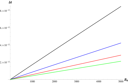
Figure 5: $\Delta t$ as a function of as a function of $B_{0}$ for different values of $B_{I}(0)$ (blue $\eta=10$, black $\eta=20$, green $\eta=30$, yellow $\eta=40$ and red $\eta=50$).

In the other side, the probability flux can be computed using Appendix C in the particular case in which $k_{x}=0$. The $n=0$ contribution to the current in the $x$ and $y$ direction reads

$$J_{x}^{(0)}=\lambda\frac{\alpha_{0}^{2}\alpha_{1}^{2}\beta\eta_{0}t}{2\hbar(\alpha_{1}^{2}+1)(\alpha_{0}^{2}+1)}\left(1-\lambda^{2}\frac{\alpha_{0}^{2}\alpha_{1}^{2}\beta^{2}}{2\hbar^{2}(\alpha_{0}^{2}+1)(\alpha_{1}^{2}+1)}\eta_{0}^{2}t^{2}\right)\sin(\omega_{(1,0)}t)$$ (55)

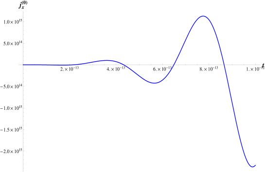
Figure 6: $n=0$ contribution of the $x$ direction of the probability flux as a function of $t$.

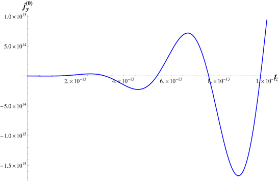
Figure 7: $n=0$ contribution of the $y$ direction of the probability flux as a function of $t$.

and for the $y$ direction

$$J_{y}^{(0)}=\lambda\frac{\alpha_{0}^{2}\alpha_{1}^{2}\beta\eta_{0}t}{2\hbar(\alpha_{1}^{2}+1)(\alpha_{0}^{2}+1)}(1-\lambda^{2}\frac{\alpha_{0}^{2}\alpha_{1}^{2}\beta^{2}}{2\hbar^{2}(\alpha_{0}^{2}+1)(\alpha_{1}^{2}+1)}\eta_{0}^{2}t^{2})\cos(\omega_{(1,0)}t)$$ (56)

Last results (or eq.(83) and eq.(84)) can be compared with the electronic current found in [27] (eq.(9)). The main difference lies in the time dependent factor of eq.(83) and eq.(84). In turn, the oscillating behavior depends on the spectral frequencies in both cases, which implies that the electronic current will not depend on the superposition of states of Bloch electrons.

From eq.(55) and eq.(56), the current flows in circular motion, as it is expected, with a modified cyclotron frequency $\omega_{(1,0)}$. If an additional constant electric field is applied along the doped graphene monolayer sheet, the result will be equivalent to monolayer doped graphene subjected to a reduced magnetic field $\widetilde{B}(t)=B(t)\sqrt{1-\theta^{2}}$, where $\theta=E/v_{f}B(t)$ (see [32], page 245). In turn, the current of eq.(81) of Appendix C will not be the net current circulating in graphene monolayer with impurities, because a time-dependent magnetic field will induce a time-dependent electric field that will points in the circumferential direction

$$\overrightarrow{E}=-\frac{1}{2}r\frac{dB}{dt}\widehat{e}_{\theta}$$ (57)

This electric field will produce, from a classical viewpoint, a  linear current density in the $\widehat{e}_{\theta}$

$$\overrightarrow{J}=-e\sqrt{\frac{2e\pi}{m}\frac{dB}{dt}}\widehat{e}_{\theta}$$ (58)

pointing in the opposite direction to the current generated by the Lorentz force. A quantum mechanical treatment is necessary to obtain the net current probability in doped graphene under a time-dependent magnetic field. It will be source of future works to study the current flux and probability transitions for an oscillating magnetic field at several orders in $\lambda$. Finally, another line of research will be the possible interacting Hamiltonian that allows possible transitions between different energy bands in the long wavelength approximation.

5 Conclusions

In this paper we have shown how to compute the Landau levels transitions of doped graphene in a time dependent magnetic field. Starting at $t=0$ from an arbitrary $m$ Landau level, we show the general behavior of the $m\pm 1$ and $m\pm 2$ Landau levels at order $\lambda^{2}$. We study the time interval at which the $m$ Landau level probability amplitude decrease to zero and its relation with the parameters of the Hamiltonian, showing minimum values of $m$ at which the $m$ Landau level vanishes. In turn, the transition from the $m$ to the $m\pm 1$ Landau level in the case in which Bloch electrons travel in the $y$ direction was analized. A three level system can be obtained in the time interval at which the $m$ Landau level vanishes with the difference that time interval do not reaches a minimum for some $m$ value. Finally, the $n=0$ and $n=1$ Landau level transition is studied in the $k_{x}=0$ regime showing that for a small time interval the electrons behave as a two-level system. The relation to the zitterbewegung effect and revivals are analized, showing similar time intervals for both effects and the probability flux due to the perturbation potential. Current probabilities are computed for low orders in $\lambda$ showing an oscillating behavior in time and where in particular negative values are found.

6 Acknowledgment

This paper was partially supported by grants of CONICET (Argentina National Research Council) and Universidad Nacional del Sur (UNS) and by ANPCyT through PICT 1770, and PIP-CONICET Nos. 114-200901-00272 and 114-200901-00068 research grants, as well as by SGCyT-UNS., E.A.G. and P.V.J. are members of CONICET. P.B. and J. S.A. are fellow researchers at this institution.

The five authors are extremely grateful to the reviewer, whose relevant observations have greatly improved the final version of this paper.

Appendix A The probability amplitude

The norm of the wave function $e^{-ik_{x}x}\varphi_{n}(\overline{\overline{y}})$ reads

$$\int\left|e^{-ik_{x}x}\varphi_{n}(\overline{\overline{y}})\right|^{2}dxd\overline{\overline{y}}=4L_{x}(\alpha_{n}^{2}+1)$$ (59)

where $2L_{x}$ is the total length in the $x$-direction of the graphene layer. From last equation, the normalization factor reads

$$N_{n}=\frac{1}{2\sqrt{L_{x}(\alpha_{n}^{2}+1)}}$$ (60)

Using the normalized wave function $e^{-ik_{x}x}\varphi_{n}$, the norm of the quantum state of eq.(13) reads

$$\int\left|\psi(x,\overline{\overline{y}},t)\right|^{2}dxd\overline{\overline{y}}=\sum\limits_{n=0}^{+\infty}\left|c_{n}(t)\right|^{2}=1$$ (61)

Then the probability amplitude for each Landau level reads

$$P_{n}(t)=\left|c_{n}(t)\right|^{2}$$ (62)

which will be used in Section 2.

Appendix B Taylor expansion

To obtain the Taylor expansion of $f_{(n,m)}(t)$ and $F_{(n,m)}^{(n^{\prime},m^{\prime})}(t)$ (eq.(25) and eq.(27)) around $t=0$ we can proceed as follows: the function $\eta(t)$ is known because depends on the applied time-dependent magnetic field $B_{I}(t)$. We can compute the Taylor expansion of this function around $t=0$

$$\eta(t)=\sum\limits_{j=0}^{+\infty}\frac{\eta_{j}}{j!}t^{j}$$ (63)

where

$$\eta_{j}=\frac{d^{j}\eta(t)}{dt^{j}}(t=0)$$ (64)

In principle we can assum that this Taylor expansion converges to $\eta(t)$ with a radius of convergence $R$, where $R\$reads

$$\frac{1}{R}=\underset{n\rightarrow\infty}{\lim}\left|\frac{\eta_{j+1}}{(j+1)\eta_{j}}\right|$$ (65)

In the other side, we can compute the Taylor expansion of $e^{-i\omega_{(n,m)}t}$ around $t=0$

$$e^{-i\omega_{(n,m)}t}=\sum\limits_{k=0}^{+\infty}\frac{(-i\omega_{(n,m)})^{k}t^{k}}{k!}$$ (66)

with an infinite radius of convergence. The Cauchy product of the two series reads

$$\left(\sum\limits_{j=0}^{+\infty}\frac{\eta_{j}}{j!}t^{j}\right)\left(\sum\limits_{k=0}^{+\infty}\frac{(-i\omega_{(n,m)})^{k}t^{k}}{k!}\right)=\sum\limits_{n=0}^{+\infty}t^{n}\sum\limits_{k=0}^{n}\frac{\eta_{k}}{k!}\frac{(-i\omega_{(n,m)})^{n-k}}{(n-k)!}$$ (67)

This product converges in radius of convergence $R$. Finally, integrating the last result we obtain the Taylor expansion of $f_{(n,m)}(t)$ around $t=0$ with radius of convergence $R$ which reads

$$f(t)=\sum\limits_{n=0}^{+\infty}\frac{t^{n+1}}{n+1}\sum\limits_{k=0}^{n}\frac{\eta_{k}}{k!}\frac{(-i\omega_{(n,m)})^{n-k}}{(n-k)!}$$ (68)

Because we want to compute the behavior of the $c_{m}^{(k)}$ coefficients near $t=0$, which is the time at which the time-dependent magnetic field is turn on, we can compute the few first terms of eq.(68)

$$f(t)=\eta_{0}t+\frac{t^{2}}{2}\left(\eta_{1}-i\omega_{(n,m)}\eta_{0}\right)+\frac{t^{3}}{3}\left(\frac{\eta_{2}}{2}-i\omega_{(n,m)}\eta_{1}-\eta_{0}\frac{\omega_{(n,m)}^{2}}{2}\right)+O(t^{4})$$ (69)

where

$$\eta_{0}=\eta(0)=\frac{B_{I}(0)}{B_{0}}$$ (70)

$$\eta_{1}=\frac{d\eta}{dt}(t=0)=\frac{1}{B_{0}}\frac{dB_{I}}{dt}(t=0)$$ (71)

and

$$\eta_{2}=\frac{d^{2}\eta}{dt^{2}}(t=0)=\frac{1}{B_{0}}\frac{d^{2}B_{I}}{dt^{2}}(t=0)$$ (72)

In a similar way, we can proceed with the Taylor expansion of eq.(27) by using the expansion of eq.(63), eq.(66) and the result of eq.(68). The product of the three expansions reads

$$\eta(t)e^{-i\omega_{(n^{\prime},m^{\prime})}t}f_{(n,m)}(t)=\sum\limits_{n=0}^{+\infty}t^{n+1}\sum\limits_{k=0}^{n}\sum\limits_{l=0}^{k}\frac{\eta_{l}}{l!}\frac{(-i\omega_{(n^{\prime},m^{\prime})})^{k-l}}{\left(n-k+1\right)(k-l)!}\left(\sum\limits_{s=0}^{n-k}\frac{\eta_{s}}{s!}\frac{(-i\omega_{(n,m)})^{n-k-s}}{(n-k-s)!}\right)$$ (73)

then the integral reads

$$F_{(n,m)}^{(n^{\prime},m^{\prime})}(t) = \int_{0}^{t}e^{-i\omega_{(n^{\prime},m^{\prime})}t^{\prime}}\eta(t^{\prime})f_{(n,m)}(t^{\prime})dt^{\prime}=\sum\limits_{n=0}^{+\infty}\frac{t^{n+2}}{n+2}\times$$

$$\sum\limits_{k=0}^{n}\sum\limits_{l=0}^{k}\frac{\eta_{l}}{l!}\frac{(-i\omega_{(n^{\prime},m^{\prime})})^{k-l}}{\left(n-k+1\right)(k-l)!}\left(\sum\limits_{s=0}^{n-k}\frac{\eta_{s}}{s!}\frac{(-i\omega_{(n,m)})^{n-k-s}}{(n-k-s)!}\right)$$

This last result is the Taylor expansion of the function $F_{(n,m)}^{(n^{\prime},m^{\prime})}(t)$ with convergence radius $R$. The first terms of this Taylor expansion read

$$F_{(n,m)}^{(n^{\prime},m^{\prime})}(t)=\frac{\eta_{0}}{2}t^{2}+\frac{\eta_{0}}{3}t^{3}\left(\frac{3}{2}\eta_{1}-i\eta_{0}\left(\omega_{(n^{\prime},m^{\prime})}+\frac{\omega_{(n,m)}}{2}\right)\right)+O(t^{4})$$ (75)

Eq.(69) and eq.(75) will be used in Section 3.

Appendix C Probability flux

The Hamiltonian of eq.(5) with an electromagnetic field can be written in a compact form as

$$H=\left[\begin{array}[]{cc}v_{f}\overrightarrow{\sigma}\cdot(-i\hbar\overrightarrow{\nabla}-e\overrightarrow{A})&UI\\ UI&\epsilon I\end{array}\right]\left[\begin{array}[]{c}\psi\\ \xi\end{array}\right]=i\hbar\frac{\partial}{\partial t}\left[\begin{array}[]{c}\psi\\ \xi\end{array}\right]$$ (76)

where $\psi$ is a two component wave function of the electrons in carbon atom and $\xi$ is a two component wave function of the electrons in the impurity atom. Last equation can be separated in two coupled differential equations for $\psi$ and $\xi$

$$v_{f}\overrightarrow{\sigma}\cdot(-i\hbar\overrightarrow{\nabla}-e\overrightarrow{A})\psi+U\xi=i\hbar\frac{\partial\psi}{\partial t}$$ (77)

and

$$U\psi+\epsilon\xi=i\hbar\frac{\partial\xi}{\partial t}$$ (78)

The probability density reads

$$\rho=\psi^{{\dagger}}\psi+\xi^{{\dagger}}\xi$$ (79)

by taking the time derivate we obtain the following continuity equation

$$\frac{\partial\rho}{\partial t}+\overrightarrow{\nabla}\left(v_{f}\psi^{{\dagger}}\overrightarrow{\sigma}\psi\right)=0$$ (80)

Then, the current probability reads

$$\overrightarrow{j}=v_{f}\psi^{{\dagger}}\overrightarrow{\sigma}\psi$$ (81)

which depends only on the two components of the electron wave function in carbon atoms.

In particular, using eq.(13) for the first and second components of the total wave function, we obtain for the current probability density components $x$ and $y$

$$j_{x}=\psi^{{\dagger}}\sigma_{x}\psi=v_{f}\sum\limits_{n=0}^{+\infty}\sum\limits_{m=0}^{+\infty}\frac{c_{m}^{\ast}(t)c_{n}(t)e^{-i\omega_{(n,m)}t}(-1)^{i}\alpha_{m}^{(i,j)}\alpha_{n}^{(i,j)}}{4L_{x}\sqrt{(\alpha_{n}^{2}+1)(\alpha_{m}^{2}+1)}}\left(\phi_{m}^{\ast}(\overline{\overline{y}})\phi_{n-1}(\overline{\overline{y}})+\phi_{m-1}^{\ast}(\overline{\overline{y}})\phi_{n}(\overline{\overline{y}})\right)$$ (82)

and

$$j_{y}=\psi^{{\dagger}}\sigma_{y}\psi=v_{f}\sum\limits_{n=0}^{+\infty}\sum\limits_{m=0}^{+\infty}\frac{ic_{m}^{\ast}(t)c_{n}(t)e^{-i\omega_{(n,m)}t}(-1)^{i}\alpha_{m}^{(i,j)}\alpha_{n}^{(i,j)}}{4L_{x}\sqrt{(\alpha_{n}^{2}+1)(\alpha_{m}^{2}+1)}}\left(\phi_{m-1}^{\ast}(\overline{\overline{y}})\phi_{n}(\overline{\overline{y}})-\phi_{m}^{\ast}(\overline{\overline{y}})\phi_{n-1}(\overline{\overline{y}})\right)$$ (83)

Integrating the coordinates and taking the real part we finally obtain the current probability in the $x$ and $y$ direction

$$J_{x}(t)=\frac{v_{f}\alpha_{0}^{2}\alpha_{1}^{2}\beta\eta_{0}t}{2\hbar(\alpha_{1}^{2}+1)(\alpha_{0}^{2}+1)}\left(1-\lambda^{2}\frac{\alpha_{0}^{2}\alpha_{1}^{2}\beta^{2}}{2\hbar^{2}(\alpha_{0}^{2}+1)(\alpha_{1}^{2}+1)}\eta_{0}^{2}t^{2}\right)\sin(\omega_{(1,0)}t)$$ (84)

and

$$J_{y}(t)=\lambda\frac{v_{f}\alpha_{0}^{2}\alpha_{1}^{2}\beta\eta_{0}t}{2\hbar(\alpha_{1}^{2}+1)(\alpha_{0}^{2}+1)}(1-\lambda^{2}\frac{\alpha_{0}^{2}\alpha_{1}^{2}\beta^{2}}{2\hbar^{2}(\alpha_{0}^{2}+1)(\alpha_{1}^{2}+1)}\eta_{0}^{2}t^{2})\cos(\omega_{(1,0)}t)$$ (85)

These results will be used in Section 5.

References

- [1] K. S. Novoselov, A. K. Geim, S. V. Morozov, D. Jiang, M. I. Katsnelson, I. V. Grigorieva, S. V. Dubonos and A. A. Firsov, Nature, 438, 197 (2005).
- [2] A.K. Geim and K. S. Novoselov, Nature Materials, 6, 183 (2007).
- [3] Y. B. Zhang, Y.W. Tan, H. L. Stormer and P. Kim, Nature, 438, 201 (2005).
- [4] A. H. Castro Neto, F. Guinea, N. M. R. Peres, K. S. Novoselov and A. K. Geim, Rev. Mod. Phys., 81, 109 (2009).
- [5] M. O. Goerbig, Rev. Mod. Phys., 83, 4, (2011).
- [6] J. McClure, Phys. Rev., 104, 666 (1956).
- [7] V. P. Gusynin and S. G. Sharapov, Phys. Rev. Lett., 95, 146801 (2005).
- [8] A. H. Castro Neto, F. Guinea and N. M. R. Peres, Phys. Rev. B, 73, 205408 (2006).
- [9] M. Koshino and E. McCann, Phys. Rev. B, 83, 165443 (2011).
- [10] Y. Zheng and T. Ando, Phys. Rev. B, 65, 245420 (2002).
- [11] R.S. Deacon, K.C. Chuang, R.J. Nicholas, K.S. Novoselov and A.K. Geim, Phys. Rev. B, 76, 81406 (2007).
- [12] G. Li and E.Y. Andrei, Nature physics, 3, 623–627 (2007).
- [13] J. G. Checkelsky, L. Li, N. P. Ong, Phys. Rev. Lett., 100, 206801 (2008).
- [14] J. G. Checkelsky, L. Li, N. P. Ong, Phys. Rev. B, 79, 115434 (2009).
- [15] G. Li, A. Luican, E. Y. Andrei, Phys. Rev. Lett., 102, 176804 (2009).
- [16] A. Luican, G. Li and E. Y. Andrei, Phys. Rev. B, 83, 041405 (2011).
- [17] M. O. Goerbig and N. Regnault, Phys. Scr., 146, 014017 (2012)
- [18] Y. Barlas, K. Yang and A. H. MacDonald, Nanotechnology, 23, 052001 (2012).
- [19] Y. Zhang, Y. Barlas and Kun Yang, Phys. Rev B, 85, 165423 (2012).
- [20] M. L. Sadowski, G. Martinez, M. Potemski, C. Berger and W. A. de Heer, Phys. Rev. Lett., 97, 266405 (2006).
- [21] Z. Jiang, E.A. Henriksen, L.C. Tung, Y.-J. Wang, M.E. Schwartz, M.Y. Han, P. Kim and H.L. Stormer, Phys. Rev. Lett., 98,197403 (2007).
- [22] K. S. Novoselov, A. K. Geim, S. V. Morozov, D. Jiang, Y. Zhang, S. V. Dubonos, I. V. Grigorieva, A. A. Firsov, Science, 306, 666-669 (2004).
- [23] S.V. Morozov, K.S. Novoselov, M.I. Katsnelson, F. Schedin, D.C. Elias, J.A. Jaszczak and A. K. Geim, Phys. Rev. Lett., 100, 016602 (2008).
- [24] M. B. Belonenko, N. G. Lebedev, N. N. Yanyushkina, and M. M. Shakirzyanov, Semiconductors, 45, 5, 628–632 (2011).
- [25] M. K. Belobenko, A. V. Pak, A. V. Zhukov and R. Bouffanais, Mod. Phys. Lett. B, 26, 28, 1250188 (2012).
- [26] J. Munarriz and F. Domínguez-Adame, Jour. Phys. A, 45, 305002 (2012).
- [27] E. Romera and F. de los Santos, Phys. Rev. B, 80, 165416 (2009).
- [28] R. Saito, G. Dresselhaus and M. S. Dresselhaus, Physical Properties of Carbon Nanotubes, (Imperial College Press, London, 1998).
- [29] W. Zhou, M. D. Kapetanakis, M. P. Prange, S. T. Pantelides, S. J. Pennycook and J. C. Idrobo, Phys. Rev. Lett., 109, 206803 (2012).
- [30] L. Ballentine, Quantum Mechanics, a Modern Development, (World Sientific, Singapore, 1998).
- [31] M. B. Belonenko, A. V. Zhukov, K. E. Nemchenko, S. Prabhakar and R. Melnik, Modern Physics Letters B, 26, 15 (2012).
- [32] S. K. Pati, T. Enoki and C. N. R. Rao, Graphene and its fascinating attributes, (World Sientific, Singapore, 2011).
- [33] K. Snizhko, V. Cheianov and S. H. Simon, Phys. Rev. B, 85, 201415 (2012).