On the uniqueness of $t\to 0_{+}$ quantum transition-state theory

Abstract

It was shown recently that there exists a true quantum transition-state theory (QTST) corresponding to the $t\to 0_{+}$ limit of a (new form of) quantum flux-side time-correlation function. Remarkably, this QTST is identical to ring-polymer molecular dynamics (RPMD) TST. Here we provide evidence which suggests very strongly that this QTST ($\equiv$ RPMD-TST) is unique, in the sense that the $t\to 0_{+}$ limit of any other flux-side time-correlation function gives either non-positive-definite quantum statistics or zero. We introduce a generalized flux-side time-correlation function which includes all other (known) flux-side time-correlation functions as special limiting cases. We find that the only non-zero $t\to 0_{+}$ limit of this function that contains positive-definite quantum statistics is RPMD-TST. Copyright (2013) American Institute of Physics. This article may be downloaded for personal use only. Any other use requires prior permission of the author and the American Institute of Physics. The following article appeared in The Journal of Chemical Physics, 139 (2013), 084116, and may be found at http://link.aip.org/link/?JCP/139/084116/1

I Introduction

Classical transition-state theory has enjoyed wide applicability and success in calculating the rates of chemical processes cha78 ; fre02 ; eyr35 ; tru96 . Its central premiseeyr35rev is the assumption that all trajectories which cross the barrier react (rather than recross). This was subsequently recognized as being equivalent to taking the short-time limit of a classical flux-side time-correlation function cha78 ; fre02 , whose long-time limit would be the exact classical rate mil74 .

Until very recently it was thought that there was no rigorous quantum generalization of classical transition-state theoryvot93 ; mil93 ; pol05 , because the $t\to 0_{+}$ limit of all known quantum flux-side time-correlation functions was zero, i.e. there was no short-time quantum rate theory which would produce the exact rate in the absence of recrossing. Nevertheless, a large variety of ‘Quantum Transition-State Theories’ (QTSTs) have been proposed gil87 ; vot89rig ; cal77 ; ben94 ; pol98 ; and09 ; vot93 ; tru96 ; gev01 ; shi02 ; pol98 ; mci13 using heuristic arguments, along with other methods of obtaining the reaction rate from short-time data mil03 ; van05 ; wan98 ; wan00 ; rom11 ; rom11adapt ; wol87 .

However, in two recent papers hel13 ; alt13 (hereinafter Paper I and Paper II) we showed that a vanishing $t\to 0_{+}$ limit arises only because the standard forms of flux-side time-correlation function use flux and side dividing surfaces that are different functions of (imaginary-time) path-integral space. When the flux and side dividing surfaces are chosen to be the same, the $t\to 0_{+}$ limit becomes non-zero.

Initially, we thought that there would be many types of computationally useful $t\to 0_{+}$ quantum TST, since there is an infinite number of ways in which one can choose a common dividing surface in path integral space. For example, one can choose the surface to be a function of just a single point (in path-integral space), in which case one recovers at $t\to 0_{+}$ the simple form of quantum TST that was introduced on heuristic grounds by Wignerwig32uber ; mil75 (and used to obtain his famous expression for parabolic-barrier tunnelling). However, this form of TST becomes negative at low temperatures,hel13 ; liu09 ; and09 because the single-point dividing surface constrains the quantum Boltzmann operator in a way that makes it non-positive-definite. To obtain positive-definite quantum statistics, it is necessary to choose dividing surfaces that are invariant under cyclic permutation of the polymer beads, since this preserves imaginary-time translation in the infinite-bead limit. Under this strict condition, the $t\to 0_{+}$ limit is guaranteed to be positive definite and, remarkably, is identical to ring-polymer molecular dynamics TST (RPMD-TST).

This last result is useful because it shows that the powerful techniques of RPMD rate theoryman05che ; man04 ; man05ref ; hab13 ; men11 ; kre13 ; ric13 ; per12 ; lix13 ; col09 ; col10 ; sul11 ; sul12 and the earlier-derived centroid TSTgil87 ; vot89rig are not heuristic guesses (as was previously thought), but are instead rigorous calculations of the instantaneous thermal quantum flux from reactants to products.

The quantum TST referred to above (i.e. RPMD-TST) is unique, in the sense that any other type of dividing surface gives non-positive-definite quantum statistics, when introduced into the ring-polymerised flux-side time-correlation function that was introduced in Paper I. However, the question then arises as to whether there are $t\to 0_{+}$ limits of different flux-side time-correlation functions, which also give positive-definite quantum statistics, but which are different from (and perhaps better than!) RPMD-TST. Here we give very strong evidence (though not a proof) that this is not the case, and that RPMD-TST is indeed the unique $t\to 0_{+}$ quantum TST.

After summarizing previous work in Sec II, we write out in Sec III the most general form of quantum flux-side dividing surface that we have been able to devise. We cannot of course prove that a more general form does not exist, but we find that the new correlation function is sufficiently general that it includes all other known flux-side time-correlation functions as special cases. In Sec IV, we take the $t\to 0_{+}$ limit of this function and obtain a set of conditions which are necessary and sufficient for the $t\to 0_{+}$ limit to be non-zero and positive-definite. We find that these conditions give RPMD-TST. Section V concludes the article.

II Review of earlier developments

To simplify the algebra, the following is presented for a one-dimensional system with coordinate $x$, mass $m$ and Hamiltonian $\hat{H}$ at an inverse temperature $\beta\equiv 1/k_{B}T$. The results generalize immediately to multi-dimensional systems, as discussed in Paper I. We begin with the Miller-Schwarz-Tromp (MST) expression for the exact quantum mechanical rate mil74 ; mil83 ,

$$k^{\rm QM}(\beta)=\lim_{t\to\infty}c_{\rm fs}^{\rm sym}(t)/Q_{\rm r}(\beta),$$ (1)

where $Q_{\rm r}(\beta)$ is the reactant partition function, and

$$c_{\rm fs}^{\rm sym}(t)={\rm Tr}\left[e^{-\beta\hat{H}/2}\hat{F}e^{-\beta\hat{H}/2}e^{i\hat{H}t/\hbar}\hat{h}e^{-i\hat{H}t/\hbar}\right]$$ (2)

where $\hat{F}$ is the quantum-mechanical flux operator

$$\hat{F}=\frac{1}{2m}\left[\delta(x-q^{\ddagger})\hat{p}+\hat{p}\delta(x-q^{\ddagger})\right]$$ (3)

and $\hat{h}$ is the heaviside operator projecting onto states in the product region, defined relative to the dividing surface $q^{\ddagger}$.

The function $c_{\rm fs}^{\rm sym}(t)$ tends smoothly to zero in the $t\to 0_{+}$ limit, vot89time ; vot93 ; mil93 which would seem to rule out the existence of a $t\to 0_{+}$ quantum transition-state theory. However, it was shown in Paper I that this behaviour arises because the flux and side dividing surfaces in Eq. (2) are different functions of path-integral space hel13 . When the two dividing surfaces are the same, the quantum flux-side time-correlation function becomes non-zero in the $t\to 0_{+}$ limit. (Note that the classical flux-side time-correlation function also tends smoothly to zero as $t\to 0_{+}$ if the flux and side dividing surfaces are different.) A simple form of quantum flux-side time-correlation function in which the two surfaces are the same is

$$C_{\rm fs}^{[1]}(t)= \int dq\int dz\int d\Delta\ h(z)\hat{F}(q)$$

$$\times\langle q-\Delta/2|e^{-\beta\hat{H}}|q+\Delta/2\rangle$$

$$\times\langle q+\Delta/2|e^{i\hat{H}t/\hbar}|z\rangle\langle z|e^{-i\hat{H}t/\hbar}|q-\Delta/2\rangle.$$ (4)

where the superscript $[1]$ indicates that the common dividing surface is a function of a single-point in path integral space. In the $t\to\infty$ limit, Eq. (4) gives the exact quantum rate. In the $t\to 0_{+}$ limit, Eq. (4) is non-zero (because the dividing surfaces are the same), and thus gives a $t\to 0_{+}$ QTST, which is found to be identical to one proposed on heuristic grounds by Wigner in 1932 wig32uber and later by Miller mil75 . Unfortunately, this form of QTST becomes negative at low temperatures, because the constrained quantum-Boltzmann operator is not positive-definite, and thus gives an erroneous description of the quantum statistics liu09 ; hel13 ; and09 .

Paper I showed that positive-definite quantum statistics can be obtained using a ring-polymerized flux-side time-correlation function of the form

$$C_{\rm fs}^{[N]}(t)= \int d{\bf q}\int d{\bf\Delta}\int d{\bf z}\ \mathcal{\hat{F}}[f({\bf q})]h[f({\bf z})]$$

$$\times\prod_{i=0}^{N-1}\langle q_{i-1}-\tfrac{1}{2}\Delta_{i-1}|e^{-\beta_{N}\hat{H}}|q_{i}+\tfrac{1}{2}\Delta_{i}\rangle$$

$$\qquad\times\langle q_{i}+\tfrac{1}{2}\Delta_{i}|e^{i\hat{H}t/\hbar}|z_{i}\rangle$$

$$\qquad\times\langle z_{i}|e^{-i\hat{H}t/\hbar}|q_{i}-\tfrac{1}{2}\Delta_{i}\rangle,$$ (5)

where the integrals extend over the whole of path-integral space ($\int d{\bf q}\equiv\int_{-\infty}^{\infty}dq_{0}\ldots\int_{-\infty}^{\infty}dq_{N-1}$ and so on), and $f({\bf q})$ is the common dividing surface, which is chosen to be invariant under cyclic permutation of the arguments ${\bf q}$ or ${\bf z}$. The ‘ring-polymer flux operator’ $\mathcal{\hat{F}}[f({\bf q})]$ describes the flux perpendicular to $f({\bf q})$, and is given by

$$\mathcal{\hat{F}}[f({\bf q})]= \frac{1}{2m}\sum_{i=0}^{N-1}\Bigg{\{}\frac{\partial f({\bf q})}{\partial q_{i}}\delta\!\left[f({\bf q})\right]\hat{p}_{i}$$

$$\qquad+\hat{p}_{i}\delta\!\left[f({\bf q})\right]\frac{\partial f({\bf q})}{\partial q_{i}}\Bigg{\}}$$ (6)

where the first term in braces is placed between $e^{-\beta_{N}\hat{H}}|q_{i}+\tfrac{1}{2}\Delta_{i}\rangle$ and $\langle q_{i}+\tfrac{1}{2}\Delta_{i}|e^{i\hat{H}t/\hbar}$, and the second term between $e^{-i\hat{H}t/\hbar}|q_{i}-\tfrac{1}{2}\Delta_{i}\rangle$ and $\langle q_{i}-\tfrac{1}{2}\Delta_{i}|e^{-\beta_{N}\hat{H}}$. We then take the limits

$$\lim_{t\to 0_{+}} \lim_{N\to\infty}C_{\rm fs}^{[N]}(t)=$$

$$\int d{\bf Q}\ \delta[f({\bf Q})]\sqrt{\frac{{\cal N}_{N}}{2\pi m\beta}}\prod_{i=0}^{N-1}\langle Q_{j-1}|e^{-\beta_{N}\hat{H}}|Q_{j}\rangle$$

$$=k_{Q}^{\ddagger}(\beta)Q_{\rm r}(\beta),$$ (7)

where

$${\cal N}_{N} =N\sum_{i=0}^{N-1}\left[\frac{\partial f({\bf Q})}{\partial Q_{i}}\right]^{2}$$ (8)

and $k_{Q}^{\ddagger}(\beta)$ is the quantum TST rate, which is guaranteed to be positive, because the cyclic-permutational invariance of $f({\bf q})$ ensures that the constrained Boltzmann operator is positive-definite. Unlike Eq. (4), Eq. (5) does not give the exact quantum rate in the limit $t\to\infty$. However, we showed in Paper II that Eq. (5) does give the exact quantum rate if there is no recrossing of the dividing surface $f({\bf q})$, and thus that $k_{Q}^{\ddagger}(\beta)$ is a good approximation to the exact quantum rate if the amount of such recrossing is small.

Remarkably,

$$k_{Q}^{\ddagger}(\beta)\equiv k_{\rm RPMD-TST}^{\ddagger}(\beta)$$ (9)

where $k_{\rm RPMD-TST}^{\ddagger}(\beta)$ is the ring-polymer molecular dynamics TST (RPMD-TST) rate, corresponding to the $t\to 0_{+}$ limit of the (classical) flux-side time-correlation function in ring-polymer space. Hence Eq. (5) gives a rigorous justification of the powerful method of RPMD-TST (and also of centroid-TST), by showing that it is a computation of the short time quantum flux (rather than merely an heuristic approach, as was previously thoughtman05che ; ric09 ; alt11 ).

As mentioned above, the dividing surface $f({\bf q})$ is invariant under cyclic permutation of the coordinates ${\bf q}$ and ${\bf z}$, meaning that $f({\bf q})$ is invariant under imaginary-time translation in the limit $N\to\infty$. In Paper I, we showed that only if this condition is met does the $t\to 0_{+}$ limit of Eq. (5) give positive-definite quantum statistics in the limit $N\to\infty$. Hence, if we start with the flux-side time-correlation function Eq. (5), the quantum TST rate $k_{Q}^{\ddagger}(\beta)\equiv k_{\rm RPMD-TST}^{\ddagger}(\beta)$ of Eq. (5) is unique, in the sense that any other $t\to 0_{+}$ limit [i.e. using a non-cyclically invariant $f({\bf q})$] does not give positive-definite quantum statistics.

III General quantum flux-side time-correlation function

Flux-side t.c.f.	$N$	$\xi_{i}^{-}$	$\xi_{i}^{+}$	$\mathcal{\hat{F}}[f({\bf q})]$	$h[g({\bf z})]$	$t\to 0_{+}$ limit
Miller-Schwarz-Tromp mil83	2	1/2	0	$\mathcal{\hat{F}}(q_{1})$	$h(z_{0})$	0
Asymmetric MST mil83	2	$\xi_{1}^{-}=1,\ \xi_{2}^{-}=0$	0	$\mathcal{\hat{F}}(q_{1})$	$h(z_{0})$	0
Kubo-transformed man05che	$\infty$	$1/N$	0	$\mathcal{\hat{F}}(q_{0})$	$\sum_{i=1}^{N-1}h(z_{i})$	0
Wigner [$C_{\rm fs}^{[1]}(t)$ of Eq. (4)]	1	1	0	$\mathcal{\hat{F}}(q_{0})$	$h(z_{0})$	Wigner TST wig32uber
$C_{\rm fs}^{[1]}(t)^{\prime}$ of Eq. (10)	1	1/2	1/2	$\mathcal{\hat{F}}(q_{0})$	$h(z_{0})$	Double-Wigner TST
Hybrid [Eq. 7 of Ref. alt13, ]	$>\!1$	$1/N$	0	$\mathcal{\hat{F}}[f({\bf q})]$	$h(z_{0})$	0
Ring-polymer [$C_{\rm fs}^{[N]}(t)$ of Eq. (5)]	$\infty$	$1/N$	0	$\mathcal{\hat{F}}[f({\bf q})]$	$h[f({\bf z})]$	RPMD-TST

Table 1: How to generate every (known) form of flux-side time-correlation function as a special case of Eq. (11). The terms $\xi_{i}^{-}$, $\xi_{i}^{+}$, $\mathcal{\hat{F}}[f({\bf q})]$ and $h[g({\bf z})]$ are defined in Eq. (11). Double-Wigner TST is the generalization of Wigner-TST that results from the $t\to 0_{+}$ limit of Eq. (4). In the hybrid and ring-polymer expressions, $f({\bf q})$ is chosen to be invariant under cyclic permutation of the coordinates $q_{i}$; RPMD-TST specialises to centroid-TST when $f({\bf q})=\sum_{i=0}^{N-1}q_{i}/N$.

The question then arises as to whether other QTSTs exist, obtained by taking the $t\to 0_{+}$ limit of other flux-side time-correlation functions, which also give positive-definite quantum statistics. It is clear that Eq. (5) is not the most general flux-side time-correlation function with such a limit because one can modify Eq. (4) to give a ‘split Wigner flux-side time-correlation function’:

$${C_{\rm fs}^{[1]}}^{\prime}(t)= \int dq\int dz\int d\Delta\int d\eta\ h(z)\mathcal{\hat{F}}(q)$$

$$\times\langle q-\Delta/2|e^{-\beta\hat{H}/2}|q+\Delta/2\rangle$$

$$\times\langle q+\Delta/2|e^{i\hat{H}t/\hbar}|z-\eta/2\rangle$$

$$\times\langle z-\eta/2|e^{-\beta\hat{H}/2}|z+\eta/2\rangle$$

$$\times\langle z+\eta/2|e^{-i\hat{H}t/\hbar}|q-\Delta/2\rangle.$$ (10)

which is easily shown to give the exact quantum rate in the $t\to\infty$ limit and to have a non-zero $t\to 0_{+}$ limit. This limit is not positive-definite, but clearly one could imagine generalizing Eq. (10) in the analogous way to which eq Eq. (5) is obtained by ring-polymerizing Eq. (4).

A form of flux-side time-correlation function which does include Eq. (10), as well as a ring-polymerized generalization of it, is

$$C_{\rm fs\neq}^{[\bm{\Xi}]}(t)= \int d{\bf q}\int d{\bf z}\int d{\bf\Delta}\int d\bm{\eta}\ \mathcal{\hat{F}}[f({\bf q})]h[g({\bf z})]$$

$$\times \prod_{i=0}^{N-1}\langle q_{i-1}-\Delta_{i-1}/2|e^{-\beta\xi_{i}^{-}\hat{H}}|q_{i}+\Delta_{i}/2\rangle$$

$$\times\langle q_{i}+\Delta_{i}/2|e^{i\hat{H}t/\hbar}|z_{i}-\eta_{i}/2\rangle$$

$$\times\langle z_{i}-\eta_{i}/2|e^{-\beta\xi_{i}^{+}\hat{H}}|z_{i}+\eta_{i}/2\rangle$$

$$\times\langle z_{i}+\eta_{i}/2|e^{-i\hat{H}t/\hbar}|q_{i}-\Delta_{i}/2\rangle.$$ (11)

Here the imaginary time-evolution has been divided into pieces of varying lengths $\xi_{i}^{\pm}\beta\hbar$, which are interspersed with forward-backward real-time propagators. To set the inverse temperature $\beta$, we impose the requirement

$$\sum_{i=0}^{N-1}\xi_{i}^{-}+\xi_{i}^{+}=1,$$ (12)

where $\xi_{i}^{\pm}\geq 0\ \forall i$. The only restrictions, at present, on the dividing surface $f({\bf q})$ are

$$\lim_{q\to\infty}f(q,q,\ldots,q)>0,$$ (13)

$$\lim_{q\to-\infty}f(q,q,\ldots,q)<0.$$ (14)

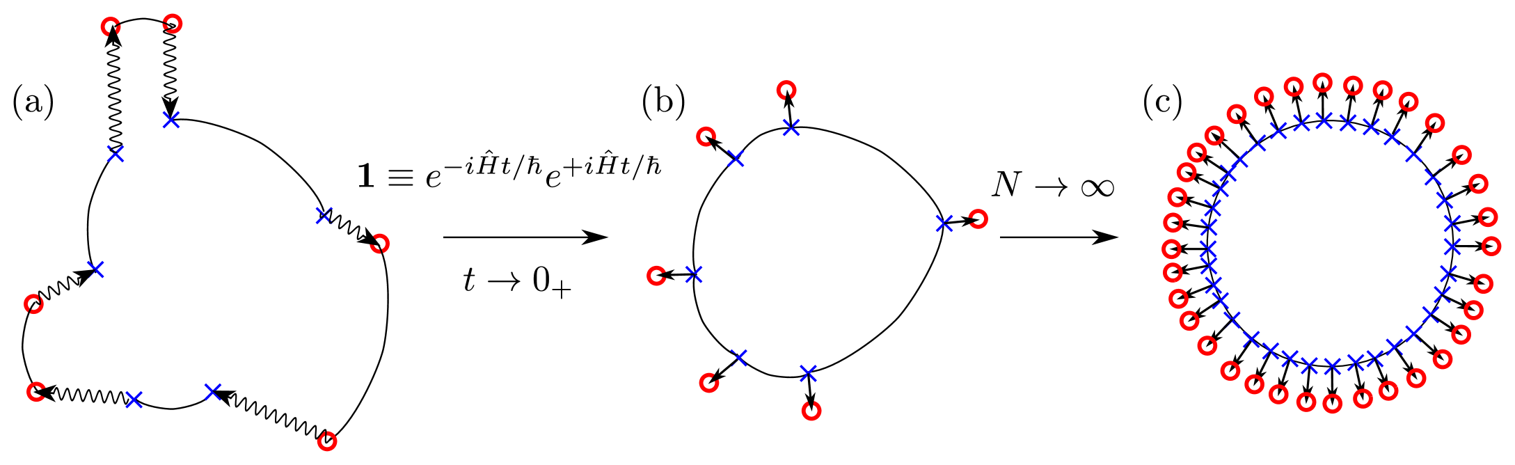
Figure 1: Diagrams showing (a) the generalized flux-side time-correlation function $C_{\rm fs\neq}^{[\bm{\Xi}]}(t)$ of Eq. (11); (b) the $t\to 0_{+}$ limit of $C_{\rm fs}^{[\bm{\Xi}]}(t)$, Eq. (24); (c) the latter for a large value of $N$. Sinusoidal lines represent real-time evolution, curved lines imaginary-time evolution, and the symbols indicate the places acted on by the flux operator $\mathcal{\hat{F}}[f({\bf q})]$ (blue crosses) and the side operator $h[g({\bf z})]$ (red circles).

and similarly for $g({\bf q})$. [These are simply the conditions that are necessary for $f({\bf q})$ and $g({\bf q})$ to distinguish reactants from products and thus do their jobs as dividing surfaces.] The subscript $\neq$ symbolises that the dividing surfaces are not necessarily equal. Equation (11) is represented diagrammatically in Fig. 1a.

The function $C_{\rm fs\neq}^{[\bm{\Xi}]}(t)$ correlates the flux averaged over a set of imaginary-time paths with the side averaged over another set of imaginary-time paths at some later time $t$. Every form of quantum flux-side time-correlation function (known to us) can be obtained either directly from $C_{\rm fs\neq}^{[\bm{\Xi}]}(t)$, using particular choices of $f({\bf q})$, $g({\bf q})$ and $\bm{\xi}$, or or by taking linear combinations of $C_{\rm fs\neq}^{[\bm{\Xi}]}(t)$ containing different values of these parameters; see Table 1. We believe that $C_{\rm fs\neq}^{[\bm{\Xi}]}(t)$ is the most general expression yet obtained for a quantum flux-side time-correlation function (before taking linear combinations), although we cannot prove that a more general expression does not exist.

IV The short-time limit

We now take the $t\to 0_{+}$ limit of Eq. (11), and determine the conditions under which this limit is non-zero and contains positive-definite quantum statistics.

IV.1 Non-zero $t\to 0_{+}$ limit

In order to calculate the short-time limit of Eq. (11) we first note that

$$\lim_{t\to 0_{+}} \langle x|e^{i\hat{H}t/\hbar}|y\rangle\langle y|e^{-i\hat{H}t/\hbar}|z\rangle$$

$$=\langle x|e^{i\hat{H}_{0}t/\hbar}|y\rangle\langle y|e^{-i\hat{H}_{0}t/\hbar}|z\rangle$$ (15)

where $\hat{H}_{0}=\hat{p}^{2}/2m$ is the free particle Hamiltonian, and that

$$\langle x|e^{-i\hat{H}_{0}t/\hbar}|y\rangle= \sqrt{\frac{m}{2\pi i\hbar t}}e^{im(x-y)^{2}/2\hbar t}$$ (16)

$$\langle x|e^{-i\hat{H}_{0}t/\hbar}\hat{p}|y\rangle= \frac{(x-y)m}{t}\sqrt{\frac{m}{2\pi i\hbar t}}e^{im(x-y)^{2}/2\hbar t}.$$ (17)

We then substitute the identity

$$e^{-\beta\xi_{i}^{+}\hat{H}}\equiv \int dy_{i}\int d\zeta_{i}\ e^{-i\hat{H}t/\hbar}|y_{i}-\zeta_{i}/2\rangle$$

$$\times\langle y_{i}-\zeta_{i}/2|e^{-\beta\xi_{i}^{+}\hat{H}}|y_{i}+\zeta_{i}/2\rangle$$

$$\times\langle y_{i}+\zeta_{i}/2|e^{i\hat{H}t/\hbar}.$$ (18)

into Eq. (11), to obtain

$$C_{\rm fs\neq}^{[\bm{\Xi}]}( t\to 0_{+})=$$

$$\lim_{t\to 0_{+}}\int d{\bf q}\int d{\bf z}\int d{\bf\Delta}\int d\bm{\eta}\int d{\bf y}\int d\bm{\zeta}$$

$$\times\ \mathcal{\hat{F}}[f({\bf q})]h[g({\bf z})]$$

$$\times\prod_{i=0}^{N-1}\langle q_{i-1}-\Delta_{i-1}/2|e^{-\beta\xi_{i}^{-}\hat{H}}|q_{i}+\Delta_{i}/2\rangle$$

$$\qquad\times\langle q_{i}+\Delta_{i}/2|e^{i\hat{H}t/\hbar}|z_{i}-\eta_{i}/2\rangle$$

$$\qquad\times\langle z_{i}-\eta_{i}/2|e^{-i\hat{H}t/\hbar}|y_{i}-\zeta_{i}/2\rangle$$

$$\qquad\times\langle y_{i}-\zeta_{i}/2|e^{-\beta\xi_{i}^{+}\hat{H}}|y_{i}+\zeta_{i}/2\rangle$$

$$\qquad\times\langle y_{i}+\zeta_{i}/2|e^{i\hat{H}t/\hbar}|z_{i}+\eta_{i}/2\rangle$$

$$\qquad\times\langle z_{i}+\eta_{i}/2|e^{-i\hat{H}t/\hbar}|q_{i}-\Delta_{i}/2\rangle.$$ (19)

The imaginary-time propagators in Eq. (19) alternate with pairs of forward-backward real-time propagators, which allows us to use Eqs. (15)–(17) to take the $t\to 0_{+}$ limit. This procedure is straightforward, but algebraically lengthy, so we give only the main steps here, relegating the details to Appendix A.

The first step (Sec. A.1) is to transform Eq. (19) to

$$C_{\rm fs\neq}^{[\bm{\Xi}]}(t)= \int d{\bf Q}\int d{\bf Z}\int d{\bf D}\ \mathcal{\hat{F}}[f({\bf Q,D})]h[g({\bf Z})]$$

$$\times \prod_{j=0}^{2N-1}\langle Q_{j-1}-D_{j-1}/2|e^{-\beta\xi_{j}\hat{H}}|Q_{j}+D_{j}/2\rangle$$

$$\times \langle Q_{j}+D_{j}/2|e^{i\hat{H}t/\hbar}|Z_{j}\rangle$$

$$\times \langle Z_{j}|e^{-i\hat{H}t/\hbar}|Q_{j}-D_{j}/2\rangle$$ (20)

where ${\bf Q}\equiv\{Q_{j}\}$, $j=0\dots 2N-1$, and similarly for ${\bf Z}$, ${\bf D}$, and

$$\xi_{2i} =\xi^{-}_{i}$$ (21)

$$\xi_{2i+1} =\xi^{+}_{i},\ \ i=0,\dots,N-1$$ (22)

i.e. we have halved the number of bra-kets in each imaginary time-slice, by doubling the number of polymer beads. Equation (20) is superficially similar to Eq. 31 of Paper I, but differs from it in the important respect that the dividing surface $f({\bf q})$ now depends on the coordinate ${\bf D}$ (in the way described in Sec. A.1). As a result the flux and side dividing surfaces are in general different functions of path integral space, even if we choose $f({\bf q})\equiv g({\bf q})$. On the basis of Paper I, one might therefore expect the $t\to 0_{+}$ limit of Eq. (20) to be zero, except for the special cases corresponding to Wigner TST and RPMD-TST (given in Table I). However, we show in Sec. A2 that the $t\to 0_{+}$ limit of Eq. (20) is always non-zero when $f({\bf q})\equiv g({\bf q})$, because the ${\bf D}$-dependence of $f({\bf Q,D})$ integrates out in this limit, to give

$$\lim_{t\to 0_{+}}C_{\rm fs}^{[\bm{\Xi}]}(t)= \frac{1}{(2\pi\hbar)^{N}}\int d{\bf Q}\int d{\bf P^{+}}\int d{\bf D^{+}}\ \delta[f({\bf Q})]S_{f}({\bf Q,P^{+}})h[S_{f}({\bf Q,P^{+}})]$$

$$\times \prod_{i=0}^{N-1}\langle Q_{2i-1}-\tfrac{1}{2\sqrt{2}}D_{i-1}^{+}|e^{-\beta\xi_{j}\hat{H}}|Q_{2i}+\tfrac{1}{2\sqrt{2}}D_{i}^{+}\rangle\langle Q_{2i}-\tfrac{1}{2\sqrt{2}}D_{i}^{+}|e^{-\beta\xi_{j}\hat{H}}|Q_{2i+1}+\tfrac{1}{2\sqrt{2}}D_{i}^{+}\rangle e^{iD^{+}_{j}P^{+}_{j}/\hbar}$$ (23)

where ${\bf P}^{+}$ and ${\bf D}^{+}$ are the $N$-dimensional vectors defined in Sec A.2, $S_{f}({\bf Q,P^{+}})$ is the flux perpendicular to $f({\bf Q})$, and the absence of a subscript $\neq$ in $C_{\rm fs}^{[\bm{\Xi}]}(t)$ indicates $f({\bf q})\equiv g({\bf q})$. Thus, in general, $f({\bf Q,D})$ acts as a time-dependent flux-dividing surface, which becomes the same as the side-dividing surface in the limit $t\to 0_{+}$ if $f({\bf q})\equiv g({\bf q})$. Clearly $f({\bf q})$ is time-independent in the special case that $\xi_{i}^{-}=1/N,\xi_{i}^{+}=0$, in which Eq. (11) reduces to Eq. (5) (see Table I).

We can tidy up Eq. (23) by integrating out $(N-1)$ of the integrals in ${\bf P}^{+}$ and ${\bf D}^{+}$ (see Sec. A.3), to obtain

$$\lim_{t\to 0_{+}}C_{\rm fs}^{[\bm{\Xi}]}(t)=\frac{1}{2\pi\hbar}\int d{\bf Q}\int d\tilde{P}_{0}\int d\tilde{D}_{0}$$

$$\times h[\tilde{P}_{0}]\frac{\tilde{P}_{0}}{m}\sqrt{B_{N}}\delta[f({\bf Q})]e^{i\tilde{D}_{0}\tilde{P}_{0}/\hbar}$$

$$\times\prod_{j=0}^{2N-1}\langle Q_{j-1}-T_{j-1\ 0}\tilde{D}_{0}/2|e^{-\beta\xi_{j}\hat{H}}|Q_{j}+T_{j0}\tilde{D}_{0}/2\rangle.$$ (24)

where $\tilde{P}_{0}$ is the momentum perpendicular to the dividing surface $f({\bf Q})$, $\tilde{D}_{0}$ describes a collective ring-opening mode, $T_{j0}$ is the weighting of the $j$th path-integral bead in the dividing surface $f({\bf Q})$ [see Eq. (54)], and $\sqrt{B_{N}}$ is a normalization constant associated with $\tilde{P}_{0}$.

IV.2 Positive-definite Boltzmann statistics

Having shown that the $t\to 0_{+}$ limit of Eq. (11) is non-zero if $f({\bf q})\equiv g({\bf q})$, we now determine the conditions on $f({\bf q})$ that give rise to positive-definite quantum statistics. The special case $\xi_{i}^{-}=1/N,\xi_{i}^{+}=0$ has already been treated in Paper I and we use the same approach here for the more general case, which is to find the condition on $f({\bf q})$ which guarantees that the integral over $\tilde{D}_{0}$ in Eq. (24) is positive in the limit $N\to\infty$. We first express the Boltzmann operator in ring polymer form,

$$\lim_{N\to\infty} \prod_{j=0}^{2N-1}\langle Q_{j-1}-T_{j-1\ 0}\tilde{D}_{0}/2|e^{-\beta\xi_{j}\hat{H}}|Q_{j}+T_{j0}\tilde{D}_{0}/2\rangle$$

$$= \prod_{j=0}^{2N-1}\sqrt{\frac{m}{2\pi\beta\xi_{j}\hbar^{2}}}$$

$$\times e^{-\beta\xi_{j}[V(Q_{j-1}-T_{j-1\ 0}\tilde{D}_{0}/2)+V(Q_{j}+T_{j0}\tilde{D}_{0}/2)]/2}$$

$$\times e^{-m[Q_{j}-Q_{j-1}+\tilde{D}_{0}(T_{j-1\ 0}+T_{j0})/2]^{2}/2\beta\xi_{j}\hbar^{2}}$$ (25)

and note that $T_{j0}\sim N^{-1/2}$, which ensures that the potential energy terms are independent of $\tilde{D}_{0}$ in the limit $N\to\infty$. Expanding the spring term,

$$\lim_{N\to\infty} \sum_{j=0}^{2N-1}\frac{m}{2\beta\xi_{j}\hbar^{2}}[Q_{j}-Q_{j-1}+\tilde{D}_{0}(T_{j-1\ 0}+T_{j0})/2]^{2}$$

$$=\lim_{N\to\infty}\sum_{j=0}^{2N-1}m[Q_{j}-Q_{j-1}]^{2}/2\beta\xi_{j}\hbar^{2}$$

$$\qquad+m[Q_{j}-Q_{j-1}]\tilde{D}_{0}(T_{j-1\ 0}+T_{j0})/2\beta\xi_{j}\hbar^{2}$$

$$\qquad+m\tilde{D}_{0}^{2}(T_{j-1\ 0}+T_{j0})^{2}/8\beta\xi_{j}\hbar^{2}$$ (26)

we see that the integral over the Boltzmann operator is guaranteed to be positive if and only if the cross-terms vanish. In other words the condition

$$\lim_{N\to\infty}\sum_{j=0}^{N-1}m[Q_{j}-Q_{j-1}]\tilde{D}_{0}(T_{j-1\ 0}+T_{j0})/2\beta\xi_{j}\hbar^{2}=0$$ (27)

must be satisfied for the Boltzmann statistics to be positive-definite. In Appendix B, we show that this condition is equivalent to requiring the dividing surface $f({\bf Q})$ to be invariant under imaginary-time translation. This was the same conclusion reached in Paper I, starting from the special case of $\xi_{i}^{-}=1/N,\xi_{i}^{+}=0$.

IV.3 Emergence of RPMD-TST

When $f({\bf q})$ is invariant under imaginary-time translation we can integrate out $\tilde{D}_{0}$ and $\tilde{P}_{0}$ (see Appendix C), to obtain

$$\lim_{t\to 0_{+}}\lim_{N\to\infty}C_{\rm fs}^{[\bm{\Xi}]}(t)= \int d{\bf Q}\ \delta[f({\bf Q})]\sqrt{\frac{\mathcal{N}_{2N}}{2\pi m\beta}}$$

$$\times\prod_{j=0}^{2N-1}\langle Q_{j-1}|e^{-\beta\xi_{j}\hat{H}}|Q_{j}\rangle$$ (28)

with

$$\mathcal{N}_{2N} =\lim_{N\to\infty}\sum_{j=0}^{2N-1}\frac{1}{4\xi_{j}}\left[\frac{\partial f({\bf Q})}{\partial Q_{j-1}}+\frac{\partial f({\bf Q})}{\partial Q_{j}}\right]^{2}$$ (29)

The integral in Eq. (28) is the generalisation of the RPMD-TST integral of Eq. (7) to unequally spaced imaginary time-slices $\xi_{j}$. Both expressions converge to the same result in the limit $N\to\infty$, i.e.

$$\lim_{t\to 0_{+}}\lim_{N\to\infty}C_{\rm fs}^{[\bm{\Xi}]}(t) =k_{Q}^{\ddagger}(\beta)Q_{\rm r}(\beta)$$

$$\equiv k_{\rm RPMD-TST}^{\ddagger}(\beta)$$ (30)

provided that $f({\bf q})\equiv g({\bf q})$ and that $f({\bf q})$ is invariant under imaginary-time translation. In other words, a positive-definite $t\to 0_{+}$ limit can arise from the general time-correlation function Eq. (11) only if $f({\bf q})$ is invariant under imaginary-time-translation (in the limit $N\to\infty$), in which case this limit is identical to that obtained from the simpler time-correlation function Eq. (31) in Paper I, namely RPMD-TST.

The above derivation can easily be generalized to multi-dimensions, by following the same procedure as that applied to Eq. (5) in Sec. V of Paper I.

V Conclusions

We have introduced an extremely general quantum flux-side time-correlation function, and found that its $t\to 0_{+}$ limit is non-zero only when the flux and side dividing surfaces are the same function of path-integral space, and that it gives positive-definite quantum statistics only when the common dividing surface is invariant to imaginary-time translation. This $t\to 0_{+}$ limit is identical to the one that was derived in Paper I starting from a simpler form of flux-side time-correlation function (a special case of the function introduced here), where it was shown to give a true $t\to 0_{+}$ quantum TST which is identical to RPMD-TST.

We cannot prove that a yet more general flux-side time-correlation function does not exist (than the one introduced here) which might support a different non-zero $t\to 0_{+}$ limit, which nevertheless gives positive-definite quantum statistics. However, given that the function introduced here includes all known flux-side time-correlation functions as special cases, we think that this is unlikely.

This article therefore provides strong evidence (although not conclusive proof) that the quantum TST of Paper I is unique, in the sense that there is no other $t\to 0_{+}$ limit which gives a non-zero quantum TST containing positive-definite quantum statistics. In other words, if one wishes to obtain an estimate of the thermal quantum rate by taking the instantaneous flux through a dividing surface, then RPMD-TST cannot be bettered.

VI Acknowledgements

TJHH is supported by a PhD studentship from the Engineering and Physical Sciences Research Council.

Appendix A Derivation of the $t\to 0_{+}$ limit of Eq. (11)

A.1 Coordinate transformation

The coordinate transform used to convert Eq. (19) to Eq. (20) is

$$Q_{j}= \left\{\begin{array}[]{ll}\tfrac{1}{2}\left(q_{i}+\Delta_{i}/2+y_{i}-\zeta_{i}/2\right),&j=2i\\ \tfrac{1}{2}\left(q_{i}-\Delta_{i}/2+y_{i}+\zeta_{i}/2\right),&j=2i+1\end{array}\right.$$ (33)

$$D_{j}= \left\{\begin{array}[]{ll}-q_{i}-\Delta_{i}/2+y_{i}-\zeta_{i}/2,&j=2i\\ q_{i}-\Delta_{i}/2-y_{i}-\zeta_{i}/2,&j=2i+1\end{array}\right.$$ (36)

$$Z_{j}= \left\{\begin{array}[]{ll}z_{i}-\eta_{i}/2,&j=2i\\ z_{i}+\eta_{i}/2,&j=2i+1\end{array}\right.$$ (39)

where $j=0,1,\ldots,2N-1$ and $i=0,1,\ldots,N-1$. The associated Jacobian is unity. Note that $f({\bf q})$ is of course unchanged by the coordinate transformation, so $f({\bf Q},{\bf D})$ in Eq. (20) depends on ${\bf Q}$ and ${\bf D}$ through the relation

$$q_{i}= \ Q_{2i}+Q_{2i+1}+(D_{2i+1}-D_{2i})/2,$$ (40)

i.e. $f({\bf Q},{\bf D})$ is not a general function of ${\bf Q}$ and ${\bf D}$, since it remains a function of only $N$ independent variables. Similarly, $g({\bf Z})$ depends on ${\bf Z}$ through

$$z_{i}= \ (Z_{2i}+Z_{2i+1})/2.$$ (41)

A.2 The $t\to 0_{+}$ limit

The $t\to 0_{+}$ limit of Eq. (20) can be obtained by a straightforward application of Eqs. (15)–(17), and is

$$\lim_{t\to 0_{+}} C_{\rm fs\neq}^{[\bm{\Xi}]}(t)=\lim_{t\to 0_{+}}\frac{1}{(2\pi\hbar)^{2N}}\int d{\bf Q}\int d{\bf P}\int d{\bf D}$$

$$\times \delta[f({\bf Q,D})]S_{f}({\bf Q,D,P})h[g({\bf Q+P}t/m)]$$

$$\times \prod_{j=0}^{2N-1}\langle Q_{j-1}-D_{j-1}/2|e^{-\beta\xi_{j}\hat{H}}|Q_{j}+D_{j}/2\rangle e^{iD_{j}P_{j}/\hbar}$$ (42)

where $P_{j}=(Z_{j}-Q_{j})m/t$, and

$$S_{f} ({\bf Q,D,P})=\frac{1}{2m}\sum_{i=1}^{N}\frac{\partial f({\bf q})}{\partial q_{i}}p_{i}$$ (43)

$$= \frac{1}{2m}\sum_{i=1}^{N}\frac{\partial f({\bf Q,D})}{\partial[Q_{2i}+Q_{2i+1}+(D_{2i+1}-D_{2i})/2]}$$

$$\times\left[P_{2i}+P_{2i+1}+\frac{m}{2t}(D_{2i+1}-D_{2i})\right]$$ (44)

with $p_{i}=(z_{i}-q_{i})m/t$.

To convert Eq. (42) to Eq. (49), we note that

$$\frac{\partial g({\bf Z})}{\partial Z_{2i}}=\frac{\partial g({\bf Z})}{\partial Z_{2i+1}},$$ (45)

[see (41)] and hence that

$$\lim_{t\to 0_{+}}g({\bf Q}+{\bf P}t/m)= g({\bf Q})+\frac{t}{m}\sum_{i=0}^{N-1}(P_{2i}+P_{2i+1})\frac{\partial g({\bf Q})}{\partial Q_{2i}}.$$ (46)

Transforming to

$$P^{+}_{i}= \ \tfrac{1}{\sqrt{2}}(P_{2i}+P_{2i+1})$$ (47)

$$P^{-}_{i}= \ \tfrac{1}{\sqrt{2}}(P_{2i}-P_{2i+1})$$ (48)

where $0\leq i\leq N-1$ and likewise for $\bf D^{+},D^{-}$, we obtain

$$\lim_{t\to 0_{+}}C_{\rm fs\neq}^{[\bm{\Xi}]}(t)= \lim_{t\to 0_{+}}\frac{1}{(2\pi\hbar)^{2N}}\int d{\bf Q}\int d{\bf P^{+}}\int d{\bf P^{-}}\int d{\bf D^{+}}\int d{\bf D^{-}}\delta[f({\bf Q,D^{-}})]S_{f}({\bf Q,D^{-},P^{+}})h[g({\bf Q}+\sqrt{2}{\bf P}^{+}t/m)]$$

$$\times\prod_{i=0}^{N-1}\Big{[}e^{iD^{+}_{i}P^{+}_{i}/\hbar}e^{iD^{-}_{i}P^{-}_{i}/\hbar}\langle Q_{2i-1}-\tfrac{1}{2\sqrt{2}}(D_{i-1}^{+}-D^{-}_{i-1})|e^{-\beta\xi_{2i}\hat{H}}|Q_{2i}+\tfrac{1}{2\sqrt{2}}(D_{i}^{+}+D_{i}^{-})\rangle$$

$$\qquad\times\langle Q_{2i}-\tfrac{1}{2\sqrt{2}}(D_{i}^{+}+D_{i}^{-})|e^{-\beta\xi_{2i+1}\hat{H}}|Q_{2i+1}+\tfrac{1}{2\sqrt{2}}(D_{i}^{+}-D_{i}^{-})\rangle\Big{]}.$$ (49)

We can then integrate out the $\bf P^{-}$ to generate $N$ Dirac delta functions in $\bf D^{-}$, such that $f({\bf Q,D^{-}})$ and $S_{f}({\bf Q,D^{-},P^{+}})$ reduce to $f({\bf Q})$ and $S_{f}({\bf Q,P^{+}})$, and Eq. (49) becomes

$$\lim_{t\to 0_{+}} C_{\rm fs\neq}^{[\bm{\Xi}]}(t)=\lim_{t\to 0_{+}}\frac{1}{(2\pi\hbar)^{N}}\int d{\bf Q}\int d{\bf P^{+}}\int d{\bf D^{+}}$$

$$\times\delta[f({\bf Q})]S_{f}({\bf Q,P^{+}})h[g({\bf Q}+\sqrt{2}{\bf P}^{+}t/m)]$$

$$\times\prod_{i=0}^{N-1}\langle Q_{2i-1}-\tfrac{1}{2\sqrt{2}}D_{i-1}^{+}|e^{-\beta\xi_{2i}\hat{H}}|Q_{2i}+\tfrac{1}{2\sqrt{2}}D_{i}^{+}\rangle$$

$$\qquad\times\langle Q_{2i}-\tfrac{1}{2\sqrt{2}}D_{i}^{+}|e^{-\beta\xi_{2i+1}\hat{H}}|Q_{2i+1}+\tfrac{1}{2\sqrt{2}}D_{i}^{+}\rangle$$

$$\qquad\times e^{iD^{+}_{i}P^{+}_{i}/\hbar}$$ (50)

It is easy to show (following the reasoning given in Sec. IIIB of Paper I) that this expression is non-zero only if $f({\bf Q})\equiv g({\bf Q})$, in which case the limit

$$\lim_{t\to 0_{+}} \delta[f({\bf Q})]h[f({\bf Q}+\sqrt{2}{\bf P}^{+}t/m)]$$

$$=\lim_{t\to 0_{+}}\delta[f({\bf Q})]h[f({\bf Q})+tS_{f}({\bf Q,P^{+}})]$$

$$=\delta[f({\bf Q})]h[S_{f}({\bf Q,P^{+}})]$$ (51)

results in Eq. (23).

A.3 Normal mode transformation

To integrate out $D_{i}^{+},\ i>0$ from Eq. (23), we transform to the coordinates

$$\tilde{P}_{j}^{\prime}= \sum_{i=0}^{N-1}P_{i}^{+}T_{2ij}^{\prime}$$ (52)

$$\tilde{D}_{j}^{\prime}= \sum_{i=0}^{N-1}D_{i}^{+}T_{2ij}^{\prime}$$ (53)

where

$$T_{i0}^{\prime}= \frac{1}{\sqrt{B_{N}}}\frac{\partial f({\bf Q})}{\partial Q_{i}},$$ (54)

$$B_{N}^{\prime}= \sum_{i=0}^{N-1}\left[\frac{\partial f({\bf Q})}{\partial Q_{2i}}\right]^{2}$$ (55)

such that $S_{f}({\bf Q,P^{+}})=\tilde{P}_{0}^{\prime}\sqrt{2B_{N}^{\prime}}$ and, from Eq. (40), $T_{2i0}^{\prime}=T_{2i+10}^{\prime}$. The other normal modes, $T_{ij}^{\prime}$, $j=1,\ldots,N-1$ are chosen to be orthogonal to $T_{i0}^{\prime}$ and their exact form need not concern us further. Unless $f({\bf Q})$ is linear in ${\bf Q}$ (such as a centroid), $T_{ij}^{\prime}$ and $B_{N}$ are functions of ${\bf Q}$. We obtain

$$\lim_{t\to 0_{+}}C_{\rm fs}^{[\bm{\Xi}]}(t)= \frac{1}{(2\pi\hbar)^{N}}\int d{\bf Q}\int d{\bf\tilde{P}^{\prime}}\int d{\bf\tilde{D}^{\prime}}\ h(\tilde{P}_{0}^{\prime})\frac{\tilde{P}_{0}^{\prime}}{m}\sqrt{B_{N}^{\prime}}\delta[f({\bf Q})]\prod_{i=0}^{N-1}e^{i\tilde{D}_{i}^{\prime}\tilde{P}_{i}^{\prime}/\hbar}$$

$$\times \prod_{j=0}^{2N-1}\langle Q_{j-1}-\tfrac{1}{2\sqrt{2}}\sum_{i=0}^{N-1}T_{j-1\ i}^{\prime}\tilde{D}_{i}^{\prime}|e^{-\beta\xi_{j}\hat{H}}|Q_{j}+\tfrac{1}{2\sqrt{2}}\sum_{i=0}^{N-1}T_{ji}^{\prime}\tilde{D}_{i}^{\prime}\rangle$$ (56)

Integrating out $\tilde{P}_{i}^{\prime},\ 1\leq i\leq N-1$ to generate Dirac delta functions in $\tilde{D}_{i}^{\prime},\ 1\leq i\leq N-1$, which are themselves then integrated out, we obtain

$$\lim_{t\to 0_{+}}C_{\rm fs}^{[\bm{\Xi}]}(t)=\frac{1}{2\pi\hbar}\int d{\bf Q}\int d\tilde{P}_{0}^{\prime}\int d\tilde{D}_{0}^{\prime}$$

$$\times h[\tilde{P}_{0}]\frac{\tilde{P}_{0}^{\prime}}{m}\sqrt{2B_{N}}\delta[f({\bf Q})]e^{i\tilde{D}_{0}^{\prime}\tilde{P}_{0}^{\prime}/\hbar}$$

$$\times\prod_{j=0}^{2N-1}\langle Q_{j-1}-\tfrac{1}{2\sqrt{2}}T_{j-1\ 0}^{\prime}\tilde{D}_{0}^{\prime}|e^{-\beta\xi_{j}\hat{H}}|Q_{j}+\tfrac{1}{2\sqrt{2}}T_{j0}^{\prime}\tilde{D}_{0}^{\prime}\rangle.$$ (57)

This transformation was made using the $N$-dimensional $\bf P^{+},D^{+}$ coordinates. To redefine the transformation from $2N$-dimensional ${\bf P},{\bf D}$ we define $\bf\tilde{P}\ \tilde{D}$ (where the absence of a prime indicates a $2N$-dimensional transformation), such that [using Eq. (40)]

$$\tilde{P}_{0}^{\prime} =\frac{\sum_{i=0}^{N-1}P_{i}^{+}\frac{\partial f({\bf Q})}{\partial Q_{2i}}}{\sqrt{\sum_{i=0}^{N-1}\left(\frac{\partial f({\bf Q})}{\partial Q_{2i}}\right)^{2}}}$$ (58)

$$=\frac{\sum_{i=0}^{2N-1}P_{i}\frac{\partial f({\bf Q})}{\partial Q_{i}}}{\sqrt{\sum_{i=0}^{2N-1}\left(\frac{\partial f({\bf Q})}{\partial Q_{i}}\right)^{2}}}$$ (59)

$$=\tilde{P}_{0}.$$ (60)

Likewise $\tilde{D}_{0}^{\prime}=\tilde{D}_{0}$. However, from Eq. (55)

$$B_{N}^{\prime} =\frac{1}{2}\sum_{i=0}^{2N-1}\left[\frac{\partial f({\bf Q})}{\partial Q_{i}}\right]^{2}$$ (61)

$$=\frac{1}{2}B_{N}$$ (62)

and it follows from this result Eq. (54) that $T_{j0}=T_{j0}^{\prime}/\sqrt{2}$. These adjustments convert Eq. (57) to Eq. (24).

Appendix B Invariance of the dividing surface to imaginary-time translation

To show that Eq. (27) is equivalent to the requirement that $f({\bf q})$ be invariant under imaginary time-translation (in the limit $N\to\infty$), we rewrite this expression in the form

$$\lim_{N\to\infty}\sum_{j=0}^{2N-1}T_{j0}\left(\frac{Q_{j+1}-Q_{j}}{\beta\hbar\xi_{j+1}}-\frac{Q_{j-1}-Q_{j}}{\beta\hbar\xi_{j}}\right)=0.$$ (63)

We then consider a shift in the imaginary-time origin by a small, positive, amount $\delta\tau$, which we represent by the operator $\mathcal{P_{+\delta\tau}}$. We then obtain

$$\lim_{N\to\infty}\mathcal{P_{+\delta\tau}}Q_{j}=Q_{j}+(Q_{j+1}-Q_{j})\delta\tau/\xi_{j+1}$$ (64)

and hence

$$\lim_{N\to\infty} \mathcal{P_{+\delta\tau}}f({\bf Q})$$

$$=\lim_{N\to\infty}f({\bf Q})+\sum_{j=0}^{2N-1}(Q_{j+1}-Q_{j})\frac{\partial f({\bf Q})}{\partial Q_{j}}\frac{\delta\tau}{\beta\hbar\xi_{j+1}},$$ (65)

Noting from Eq. (54) that $\partial f({\bf Q})/\partial Q_{j}=\sqrt{B_{N}}T_{j0}$, we see that the second term on the RHS of Eq. (65) is proportional to the first term on the LHS of Eq. (63). Using similar reasoning, we find that the second term on the LHS of Eq. (63) is proportional to $-\lim_{N\to\infty}\mathcal{P_{-\delta\tau}}f({\bf Q})$, where $\mathcal{P_{-\delta\tau}}$ denotes a shift in the imaginary-time origin by a small, negative, amount $-\delta\tau$. Eq. (63) is thus equivalent to the condition

$$\lim_{N\to\infty}\mathcal{P_{+\delta\tau}}f({\bf Q})-\mathcal{P_{-\delta\tau}}f({\bf Q})=0,$$ (66)

i.e. that the dividing surface $f({\bf Q})$ is invariant to imaginary-time-translation in the limit $N\to\infty$.

Appendix C Integrating out the ring-opening coordinate

When Eq. (27) is satisfied, the only contribution to the imaginary-time path-integral from $D_{0}$ in the limit $N\to\infty$ is the term ${m\tilde{D}_{0}^{2}}A({\bf Q})/{2\beta\hbar^{2}}$, in which

$$A({\bf Q}) =\lim_{N\to\infty}\sum_{j=0}^{2N-1}\frac{1}{4\xi_{j}}\left[T_{j-1\ 0}+T_{j0}\right]^{2}$$ (67)

$$=\lim_{N\to\infty}\frac{1}{B_{N}}\sum_{j=0}^{2N-1}\frac{1}{4\xi_{j}}\left[\frac{\partial f({\bf Q})}{\partial Q_{j-1}}+\frac{\partial f({\bf Q})}{\partial Q_{j}}\right]^{2}$$ (68)

and where the last line follows from the definition of $T_{j0}$ in Appendix A. The integral over $\tilde{D}_{0}$ in Eq. (24) is then easily evaluated to give

$$\lim_{t\to 0_{+}} C_{\rm fs}^{[\bm{\Xi}]}(t)=\frac{1}{2\pi\hbar}\int d{\bf Q}\int d\tilde{P}_{0}\ h[\tilde{P}_{0}]\frac{\tilde{P}_{0}}{m}\sqrt{B_{N}}\delta[f({\bf Q})]$$

$$\times\sqrt{\frac{2\pi\beta\hbar^{2}}{mA({\bf Q})}}e^{-\beta\tilde{P}_{0}^{2}/2mA({\bf Q})}\prod_{j=0}^{2N-1}\langle Q_{j-1}|e^{-\beta\xi_{j}\hat{H}}|Q_{j}\rangle$$ (69)

and integration over $\tilde{P}_{0}$ gives Eq. (28).

References

- (1) D. Chandler, J. Chem. Phys. 68 (1978), 2959.
- (2) D. Frenkel and B. Smit, Understanding Molecular Simulation, Academic Press (2002).
- (3) H. Eyring, J. Chem. Phys. 3 (1935), 107.
- (4) D. G. Truhlar, B. C. Garrett and S. J. Klippenstein, J. Phys. Chem. 100 (1996), 12771.
- (5) H. Eyring, Chem. Rev. 17 (1935), 65.
- (6) This article is concerned with configuration-space TST, not the formally exact phase-space TST as discussed in S. Wiggins, L. Wiesenfeld, C. Jaffé and T. Uzer, Phys. Rev. Lett. 86 (2001), 5478.
- (7) W. H. Miller, J. Chem. Phys. 61 (1974), 1823.
- (8) G. A. Voth, J. Phys. Chem. 97 (1993), 8365.
- (9) W. H. Miller, Acc. Chem. Res. 26 (1993), 174.
- (10) E. Pollak and P. Talkner, Chaos 15 (2005), 026116.
- (11) M. J. Gillan, J. Phys. C 20 (1987), 3621.
- (12) G. A. Voth, D. Chandler and W. H. Miller, J. Chem. Phys. 91 (1989), 7749.
- (13) C. G. Callan and S. Coleman, Phys. Rev. D 16 (1977), 1762.
- (14) V. A. Benderskii, D. E. Makarov and C. A. Wight, Chemical Dynamics at Low Temperatures, volume 88 of Adv. Chem. Phys., Wiley, New York (1994).
- (15) E. Pollak and J.-L. Liao, J. Chem. Phys. 108 (1998), 2733.
- (16) S. Andersson, G. Nyman, A. Arnaldsson, U. Manthe and H. Jónsson, J. Phys. Chem. A 113 (2009), 4468.
- (17) E. Geva, Q. Shi and G. A. Voth, J. Chem. Phys. 115 (2001), 9209.
- (18) Q. Shi and E. Geva, J. Chem. Phys. 116 (2002), 3223.
- (19) E. M. McIntosh, K. T. Wikfeldt, J. Ellis, A. Michaelides and W. Allison, J. Phys. Chem. Lett. 4 (2013), 1565.
- (20) W. H. Miller, Y. Zhao, M. Ceotto and S. Yang, J. Chem. Phys. 119 (2003), 1329.
- (21) J. Vaníček, W. H. Miller, J. F. Castillo and F. J. Aoiz, J. Chem. Phys. 123 (2005), 054108.
- (22) H. Wang, X. Sun and W. H. Miller, J. Chem. Phys. 108 (1998), 9726.
- (23) H. Wang, M. Thoss and W. H. Miller, J. Chem. Phys. 112 (2000), 47.
- (24) J. B. Rommel, T. P. M. Goumans and J. Kästner, J. Chem. Theor. Comput. 7 (2011), 690.
- (25) J. B. Rommel and J. Kästner, J. Chem. Phys. 134 (2011), 184107.
- (26) P. G. Wolynes, J. Chem. Phys. 87 (1987), 6559.
- (27) T. J. H. Hele and S. C. Althorpe, J. Chem. Phys. 138 (2013), 084108.
- (28) S. C. Althorpe and T. J. H. Hele, J. Chem. Phys. 139 (2013), 084115.
- (29) E. Wigner, Z. Phys. Chem. B 19 (1932), 203.
- (30) W. H. Miller, J. Chem. Phys. 62 (1975), 1899.
- (31) J. Liu and W. H. Miller, J. Chem. Phys. 131 (2009), 074113.
- (32) I. R. Craig and D. E. Manolopoulos, J. Chem. Phys. 122 (2005), 084106.
- (33) I. R. Craig and D. E. Manolopoulos, J. Chem. Phys. 121 (2004), 3368.
- (34) I. R. Craig and D. E. Manolopoulos, J. Chem. Phys. 123 (2005), 034102.
- (35) S. Habershon, D. E. Manolopoulos, T. E. Markland and T. F. Miller, Annu. Rev. Phys. Chem. 64 (2013), 387, pMID: 23298242.
- (36) A. R. Menzeleev, N. Ananth and T. F. Miller III, J. Chem. Phys. 135 (2011), 074106.
- (37) J. S. Kretchmer and T. F. Miller III, J. Chem. Phys. 138 (2013), 134109.
- (38) J. O. Richardson and M. Thoss, J. Chem. Phys. 139 (2013), 031102.
- (39) R. Pérez de Tudela, F. J. Aoiz, Y. V. Suleimanov and D. E. Manolopoulos, J. Phys. Chem. Lett. 3 (2012), 493.
- (40) Y. Li, Y. V. Suleimanov, M. Yang, W. H. Green and H. Guo, J. Phys. Chem. Lett. 4 (2013), 48.
- (41) R. Collepardo-Guevara, Y. V. Suleimanov and D. E. Manolopoulos, J. Chem. Phys. 130 (2009), 174713.
- (42) R. Collepardo-Guevara, Y. V. Suleimanov and D. E. Manolopoulos, J. Chem. Phys. 133 (2010), 049902.
- (43) Y. V. Suleimanov, R. Collepardo-Guevara and D. E. Manolopoulos, J. Chem. Phys. 134 (2011), 044131.
- (44) Y. V. Suleimanov, The Journal of Physical Chemistry C 116 (2012), 11141.
- (45) Note that direct application of RPMD rate theory [i.e. exact classical rate theory applied in the extended (fictitious) ring-polymer space] gives a lower bound to the RPMD-TST result, and thus a lower bound to the instantaneous quantum flux through the ring-polymer dividing surface.
- (46) W. H. Miller, S. D. Schwartz and J. W. Tromp, J. Chem. Phys. 79 (1983), 4889.
- (47) G. A. Voth, D. Chandler and W. H. Miller, J. Phys. Chem. 93 (1989), 7009.
- (48) See Sec. IV B of Paper I (Ref. hel13 ) for details.
- (49) J. O. Richardson and S. C. Althorpe, J. Chem. Phys. 131 (2009), 214106.
- (50) S. C. Althorpe, J. Chem. Phys. 134 (2011), 114104.
- (51) The derivation presented here assumes a single potential energy surface. It could also be performed for a system with multiple potential energy surfaces by treating the potential in the manner of M. H Alexander, Chem. Phys. Lett. 347 (2001), 436.
- (52) One can evaluate the short-time limit of Eq. (11) without the insertion of the unit operators, but their use greatly simplifies the subsequent algebra.
- (53) For equally spaced imaginary-time intervals, the leading non-zero term in the potential goes as , giving more rapid convergence with respect to than the general case of unequally-spaced intervals discussed in the text.