¹¹institutetext: Leiden Observatory, Leiden University, PO Box 9513, 2300 RA Leiden, The Netherlands^†^†thanks: ¹¹email: yildiz@strw.leidenuniv.nl ²²institutetext: S.N. Bose National Centre for Basic Sciences, Salt Lake, Kolkata, 700098, India ³³institutetext: Jet Propulsion Laboratory, California Institute of Technology, 4800 Oak Grove Drive, Pasadena CA, 91109, USA ⁴⁴institutetext: Max Planck Institut für Extraterrestrische Physik, Giessenbachstrasse 1, 85748 Garching, Germany ⁵⁵institutetext: Harvard-Smithsonian Center for Astrophysics, 60 Garden Street, Cambridge, MA 02138, USA ⁶⁶institutetext: Department of Astronomy, LGRT 619, University of Massachusetts, 710 North Pleasant Street, Amherst, MA 01003, USA ⁷⁷institutetext: Dept. of Earth & Space Sciences, Chalmers University of Technology, Onsala Space Observatory, SE-439 92 Onsala, Sweden ⁸⁸institutetext: LERMA & UMR8112 du CNRS, Observatoire de Paris, 61 Av. de l’Observatoire, 75014, Paris, France ⁹⁹institutetext: Department of Astronomy, University of Michigan, 500 Church Street, Ann Arbor, MI 48109-1042, USA ¹⁰¹⁰institutetext: School of Physics and Astronomy, University of Leeds, Leeds LS2 9JT, UK ¹¹¹¹institutetext: INAF-Osservatorio Astrofisico di Arcetri, Largo E. Fermi 5, I-50125 Firenze, Italy ¹²¹²institutetext: Departments of Chemistry, Astronomy, and Physics, The University of Virginia, Charlottesville, Virginia, USA ¹³¹³institutetext: California Institute of Technology, Cahill Center for Astronomy and Astrophysics 301-17, Pasadena, CA 91125, USA ¹⁴¹⁴institutetext: LRA/LERMA, CNRS, UMR8112, Observatoire de Paris & École Normale Supérieure, 24 rue Lhomond, 75231 Paris Cedex 05, France

Deep observations of O₂ toward a low-mass protostar with Herschel-HIFI^†^†thanks: Herschel is an ESA space observatory with science instruments provided by European-led Principal Investigator consortia and with important participation from NASA.

Umut A. Yıldız Deep observations of O₂ toward a low-mass protostar with Herschel-HIFI^†^†thanks: Herschel is an ESA space observatory with science instruments provided by European-led Principal Investigator consortia and with important participation from NASA.Deep observations of O₂ toward a low-mass protostar with Herschel-HIFI^†^†thanks: Herschel is an ESA space observatory with science instruments provided by European-led Principal Investigator consortia and with important participation from NASA. Kinsuk Acharyya Deep observations of O₂ toward a low-mass protostar with Herschel-HIFI^†^†thanks: Herschel is an ESA space observatory with science instruments provided by European-led Principal Investigator consortia and with important participation from NASA.Deep observations of O₂ toward a low-mass protostar with Herschel-HIFI^†^†thanks: Herschel is an ESA space observatory with science instruments provided by European-led Principal Investigator consortia and with important participation from NASA. Paul F. Goldsmith Deep observations of O₂ toward a low-mass protostar with Herschel-HIFI^†^†thanks: Herschel is an ESA space observatory with science instruments provided by European-led Principal Investigator consortia and with important participation from NASA.Deep observations of O₂ toward a low-mass protostar with Herschel-HIFI^†^†thanks: Herschel is an ESA space observatory with science instruments provided by European-led Principal Investigator consortia and with important participation from NASA. Ewine F. van Dishoeck Deep observations of O₂ toward a low-mass protostar with Herschel-HIFI^†^†thanks: Herschel is an ESA space observatory with science instruments provided by European-led Principal Investigator consortia and with important participation from NASA.Deep observations of O₂ toward a low-mass protostar with Herschel-HIFI^†^†thanks: Herschel is an ESA space observatory with science instruments provided by European-led Principal Investigator consortia and with important participation from NASA.Deep observations of O₂ toward a low-mass protostar with Herschel-HIFI^†^†thanks: Herschel is an ESA space observatory with science instruments provided by European-led Principal Investigator consortia and with important participation from NASA.Deep observations of O₂ toward a low-mass protostar with Herschel-HIFI^†^†thanks: Herschel is an ESA space observatory with science instruments provided by European-led Principal Investigator consortia and with important participation from NASA. Gary Melnick Deep observations of O₂ toward a low-mass protostar with Herschel-HIFI^†^†thanks: Herschel is an ESA space observatory with science instruments provided by European-led Principal Investigator consortia and with important participation from NASA.Deep observations of O₂ toward a low-mass protostar with Herschel-HIFI^†^†thanks: Herschel is an ESA space observatory with science instruments provided by European-led Principal Investigator consortia and with important participation from NASA. Ronald Snell René Liseau Deep observations of O₂ toward a low-mass protostar with Herschel-HIFI^†^†thanks: Herschel is an ESA space observatory with science instruments provided by European-led Principal Investigator consortia and with important participation from NASA.Deep observations of O₂ toward a low-mass protostar with Herschel-HIFI^†^†thanks: Herschel is an ESA space observatory with science instruments provided by European-led Principal Investigator consortia and with important participation from NASA.Deep observations of O₂ toward a low-mass protostar with Herschel-HIFI^†^†thanks: Herschel is an ESA space observatory with science instruments provided by European-led Principal Investigator consortia and with important participation from NASA.Deep observations of O₂ toward a low-mass protostar with Herschel-HIFI^†^†thanks: Herschel is an ESA space observatory with science instruments provided by European-led Principal Investigator consortia and with important participation from NASA. Jo-Hsin Chen Deep observations of O₂ toward a low-mass protostar with Herschel-HIFI^†^†thanks: Herschel is an ESA space observatory with science instruments provided by European-led Principal Investigator consortia and with important participation from NASA.Deep observations of O₂ toward a low-mass protostar with Herschel-HIFI^†^†thanks: Herschel is an ESA space observatory with science instruments provided by European-led Principal Investigator consortia and with important participation from NASA. Laurent Pagani Deep observations of O₂ toward a low-mass protostar with Herschel-HIFI^†^†thanks: Herschel is an ESA space observatory with science instruments provided by European-led Principal Investigator consortia and with important participation from NASA.Deep observations of O₂ toward a low-mass protostar with Herschel-HIFI^†^†thanks: Herschel is an ESA space observatory with science instruments provided by European-led Principal Investigator consortia and with important participation from NASA. Edwin Bergin Deep observations of O₂ toward a low-mass protostar with Herschel-HIFI^†^†thanks: Herschel is an ESA space observatory with science instruments provided by European-led Principal Investigator consortia and with important participation from NASA.Deep observations of O₂ toward a low-mass protostar with Herschel-HIFI^†^†thanks: Herschel is an ESA space observatory with science instruments provided by European-led Principal Investigator consortia and with important participation from NASA. Paola Caselli Deep observations of O₂ toward a low-mass protostar with Herschel-HIFI^†^†thanks: Herschel is an ESA space observatory with science instruments provided by European-led Principal Investigator consortia and with important participation from NASA.Deep observations of O₂ toward a low-mass protostar with Herschel-HIFI^†^†thanks: Herschel is an ESA space observatory with science instruments provided by European-led Principal Investigator consortia and with important participation from NASA.Deep observations of O₂ toward a low-mass protostar with Herschel-HIFI^†^†thanks: Herschel is an ESA space observatory with science instruments provided by European-led Principal Investigator consortia and with important participation from NASA.Deep observations of O₂ toward a low-mass protostar with Herschel-HIFI^†^†thanks: Herschel is an ESA space observatory with science instruments provided by European-led Principal Investigator consortia and with important participation from NASA. Eric Herbst Deep observations of O₂ toward a low-mass protostar with Herschel-HIFI^†^†thanks: Herschel is an ESA space observatory with science instruments provided by European-led Principal Investigator consortia and with important participation from NASA.Deep observations of O₂ toward a low-mass protostar with Herschel-HIFI^†^†thanks: Herschel is an ESA space observatory with science instruments provided by European-led Principal Investigator consortia and with important participation from NASA. Lars E. Kristensen Deep observations of O₂ toward a low-mass protostar with Herschel-HIFI^†^†thanks: Herschel is an ESA space observatory with science instruments provided by European-led Principal Investigator consortia and with important participation from NASA.Deep observations of O₂ toward a low-mass protostar with Herschel-HIFI^†^†thanks: Herschel is an ESA space observatory with science instruments provided by European-led Principal Investigator consortia and with important participation from NASA. Ruud Visser Deep observations of O₂ toward a low-mass protostar with Herschel-HIFI^†^†thanks: Herschel is an ESA space observatory with science instruments provided by European-led Principal Investigator consortia and with important participation from NASA.Deep observations of O₂ toward a low-mass protostar with Herschel-HIFI^†^†thanks: Herschel is an ESA space observatory with science instruments provided by European-led Principal Investigator consortia and with important participation from NASA. Dariusz C. Lis Deep observations of O₂ toward a low-mass protostar with Herschel-HIFI^†^†thanks: Herschel is an ESA space observatory with science instruments provided by European-led Principal Investigator consortia and with important participation from NASA.Deep observations of O₂ toward a low-mass protostar with Herschel-HIFI^†^†thanks: Herschel is an ESA space observatory with science instruments provided by European-led Principal Investigator consortia and with important participation from NASA. Maryvonne Gerin Deep observations of O₂ toward a low-mass protostar with Herschel-HIFI^†^†thanks: Herschel is an ESA space observatory with science instruments provided by European-led Principal Investigator consortia and with important participation from NASA.Deep observations of O₂ toward a low-mass protostar with Herschel-HIFI^†^†thanks: Herschel is an ESA space observatory with science instruments provided by European-led Principal Investigator consortia and with important participation from NASA.

(Draft: xxxx xx xx)

Abstract

Context. According to traditional gas-phase chemical models, O₂ should be abundant in molecular clouds, but until recently, attempts to detect interstellar O₂ line emission with ground- and space-based observatories have failed.

Aims. Following the multi-line detections of O₂ with low abundances in the Orion and $\rho$ Oph A molecular clouds with Herschel, it is important to investigate other environments, and we here quantify the O₂ abundance near a solar-mass protostar.

Methods. Observations of molecular oxygen, O₂, at 487 GHz toward a deeply embedded low-mass Class 0 protostar, NGC~1333-IRAS~4A, are presented, using the Heterodyne Instrument for the Far Infrared (HIFI) on the Herschel Space Observatory. Complementary data of the chemically related NO and CO molecules are obtained as well. The high spectral resolution data are analysed using radiative transfer models to infer column densities and abundances, and are tested directly against full gas-grain chemical models.

Results. The deep HIFI spectrum fails to show O₂ at the velocity of the dense protostellar envelope, implying one of the lowest abundance upper limits of O₂/H₂ at $\leq$ 6 $\times$ 10^-9 (3 $\sigma$ ). The O₂/CO abundance ratio is less than 0.005. However, a tentative (4.5 $\sigma$ ) detection of O₂ is seen at the velocity of the surrounding NGC 1333 molecular cloud, shifted by 1 km s^-1 relative to the protostar. For the protostellar envelope, pure gas-phase models and gas-grain chemical models require a long pre-collapse phase ( $\sim$ 0.7–1 $\times$ 10⁶ years), during which atomic and molecular oxygen are frozen out onto dust grains and fully converted to H₂O, to avoid overproduction of O₂ in the dense envelope. The same model also reproduces the limits on the chemically related NO molecule if hydrogenation of NO on the grains to more complex molecules such as NH₂OH, found in recent laboratory experiments, is included. The tentative detection of O₂ in the surrounding cloud is consistent with a low-density PDR model with small changes in reaction rates.

Conclusions. The low O₂ abundance in the collapsing envelope around a low-mass protostar suggests that the gas and ice entering protoplanetary disks is very poor in O₂.

Key Words.:

Astrochemistry — Stars: formation — ISM: abundances — ISM: molecules — ISM: individual objects: NGC~1333~IRAS~4A

1 Introduction

Even though molecular oxygen (O₂) has a simple chemical structure, it remains difficult to detect in the interstellar medium after many years of searches (Goldsmith et al. 2011, and references therein). Oxygen is the third most abundant element in the Universe, after hydrogen and helium, which makes it very important in terms of understanding the formation and evolution of the chemistry in astronomical sources.

Pure gas-phase chemistry models suggest a steady-state abundance of $X$ (O₂) $\approx$ 7 $\times$ 10^-5 relative to H₂ (e.g., Table 9 of Woodall et al. 2007), however observations show that the abundance is several orders of magnitude lower than these model predictions. Early (unsuccessful) ground-based searches of O₂ were done through the ¹⁶O¹⁸O isotopologue (Goldsmith et al. 1985; Pagani et al. 1993), for which some of the lines fall in a transparent part of the atmosphere. Due to the oxygen content of the Earth’s atmosphere, it is however best to observe O₂ from space. Two previous space missions, the Submillimeter Wave Astronomy Satellite (SWAS; Melnick et al. 2000) and the Odin Satellite (Nordh et al. 2003) were aimed at detecting and studying interstellar molecular oxygen through specific transitions. SWAS failed to obtain a definitive detection of O₂ at 487 GHz toward nearby clouds (Goldsmith et al. 2000), whereas Odin observations of O₂ at 119 GHz gave upper limits of $\leq$ 10^-7 (Pagani et al. 2003), except for the $\rho$ Ophiuchi A cloud ( $X$ (O₂) $\sim$ 5 $\times$ 10^-8; Larsson et al. 2007).

The Herschel Space Observatory provides much higher spatial resolution and sensitivity than previous missions and therefore allows very deep searches for O₂. Recently, Herschel-HIFI provided firm multi-line detections of O₂ in the Orion and $\rho$ Oph A molecular clouds (Goldsmith et al. 2011; Liseau et al. 2012). The abundance was found to range from $X$ (O₂) $\simeq$ 10^-6 (in Orion) to $X$ (O₂) $\simeq$ 5 $\times$ 10^-8 (in $\rho$ Oph A). The interpretation of the low abundance is that oxygen atoms are frozen out onto grains and transformed into water ice that coats interstellar dust, leaving little atomic O in the gas to produce O₂ (Bergin et al. 2000). So far, O₂ has only been found in clouds where (external) starlight has heated the dust and prevented atomic O from sticking onto the grains and being processed into H₂O as predicted by theory (Hollenbach et al. 2009) or where O₂ is enhanced in postshock gas (Goldsmith et al. 2011). Not every warm cloud has O₂, however. Melnick et al. (2012) report a low upper limit on gaseous O₂ toward the dense Orion Bar photon-dominated region (PDR).

Refer to caption — Figure 1: Spitzer/IRAC1 (Gutermuth et al. 2008) and CO 6–5 contours (Yıldız et al. 2012) are overlaid to illustrate the NGC 1333 IRAS 4A and 4B protostars. The white circle in the center represents the observed HIFI beam of 44 $\arcsec$ centred on IRAS 4A, illustrating that it partially overlaps with the outer part of the IRAS 4B envelope. The contours indicate the outflows, with levels starting from 15 K km s^-1 with an increasing step size of 30 K km s^-1. Blue and red velocity ranges are selected from –20 to 2.7 and from 10.5 to 30 km s^-1, respectively. The black dot on upper right corner shows the beam size of the CO 6–5 data.

Although the detection of O₂ in some molecular clouds is significant, these data tell little about the presence of O₂ in regions where solar systems may form. It is therefore important to also make deep searches for O₂ near solar-mass protostars to understand the origin of molecular oxygen in protoplanetary disks and eventually (exo-)planetary atmospheres. Even though the bulk of the O₂ in the Earth’s atmosphere arises from microorganisms, the amount of O₂ that could be delivered by cometesimal impacts needs to be quantified. In the present paper, a nearby low-mass deeply embedded protostar, NGC 1333 IRAS 4A, is targeted, which has one of the highest line of sight hydrogen column densities of $N$ (H₂) $\sim$ 10²⁴ cm^-2 derived from dust modeling (Jørgensen et al. 2002; Kristensen et al. 2012). Since the Herschel beam size at 487 GHz is a factor of $\sim$ 6 smaller than that of SWAS, Herschel is much more sensitive to emission from these compact sources. Protostars also differ from dense clouds or PDRs by the fact that a significant fraction of the dust is heated internally by the protostellar luminosity to temperatures above those needed to sublimate O and O₂.

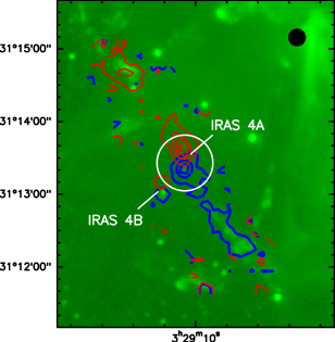
NGC~1333~IRAS~4A is located in the southeast part of the NGC 1333 region, together with IRAS 4B (henceforth IRAS~4A and IRAS~4B). A distance of 235 $\pm$ 18 pc is adopted based on VLBI parallax measurements of water masers in the nearby source SVS 13 (Hirota et al. 2008). Both objects are classified as deeply-embedded Class 0 low-mass protostars (André & Montmerle 1994) and are well-studied in different molecular lines such as CO, SiO, H₂O and CH₃OH (e.g., Blake et al. 1995; Lefloch et al. 1998; Bottinelli et al. 2007; Yıldız et al. 2012; Kristensen et al. 2010). Figure 1 shows a CO $J$ =6–5 contour map obtained with APEX (Yıldız et al. 2012) overlaid on a Spitzer/IRAC1 (3.6 $\mu{\rm m}$ ) image (Gutermuth et al. 2008). Both IRAS 4A and IRAS 4B have high-velocity outflows seen at different inclinations. The projected separation between the centers of IRAS 4A and IRAS 4B is 31 $\arcsec$ ( $\sim$ 7300 AU). The source IRAS4A was chosen for the deep O₂ search because of its chemical richness and high total column density. In contrast to many high-mass protostars, it has the advantage that even very sensitive spectra do not show line confusion.

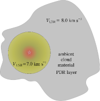
On a larger scale, early millimeter observations of CO and ¹³CO $J$ =1–0 by Loren (1976) and Liseau et al. (1988) found two (possibly colliding) clouds in the NGC 1333 region, with velocities separated by up to 2 km s^-1. Černis (1990) used extinction mapping in the NGC 1333 region to confirm the existence of two different clouds. The IRAS 4A protostellar envelope is centred at the lower velocity around $V_{\rm LSR}$ =7.0 km s^-1, whereas the lower (column) density cloud appears around $V_{\rm LSR}$ =8.0 km s^-1. The high spectral resolution of our data allows O₂ to be probed in both clouds. Optically thin isotopologue data of C¹⁸O $J$ =1–0 up to $J$ =5–4 are used to characterize the conditions in the two components. Note that these velocities do not overlap with those of the red outflow lobe, which start at $V_{\rm LSR}$ =+10.5 km s^-1.

We present here the first sensitive observations of the O₂ 3₃–1₂ 487 GHz line towards a deeply embedded low-mass Class 0 protostar, observed with Herschel-HIFI. Under a wide range of conditions, the O₂ line at 487 GHz is the strongest, therefore this line is selected for long integration. The data are complemented by ground-based observations of CO isotopologues and NO using the IRAM 30m and JCMT telescopes. The CO data are used to characterize the kinematics and physical conditions in the clouds as well as the column of gas where CO is not frozen out. Since the O₂ ice has a very similar binding energy as the CO ice, either in pure or mixed form (Collings et al. 2004; Acharyya et al. 2007), CO provides a good reference for O₂. NO is chosen because it is a related species that could help to constrain the chemistry of O₂. In the gas, O₂ can be produced from atomic O through the reaction (Herbst & Klemperer 1973; Black & Smith 1984)

{\rm O+OH\to O_{2}+H}

(1)

with rate constants measured by Carty et al. (2006). The nitrogen equivalent of Eq. (1) produces NO through

{\rm N+OH\to NO+H.}

(2)

Table 1: Overview of the observed lines.

Molecule	Transition	$E_{\mathrm{u}}/k_{\mathrm{B}}$	$A_{\rm ul}$	Frequency
		[K]	[s^-1]	[GHz]
O₂	$N_{J}$ =3₃–1₂	26.4	8.657 $\times$ 10^-9	487.2492640
C¹⁸O	$J$ =1–0	15.3	6.266 $\times$ 10^-8	109.7821734
C¹⁸O	$J$ =3–2	31.6	2.172 $\times$ 10^-6	329.3305525
C¹⁸O	$J$ =5–4	79.0	1.062 $\times$ 10^-5	548.8310055
NO (1)	$J$ =5/2–3/2, $F$ =3/2–1/2	19.3	1.387 $\times$ 10^-6	250.8169540
NO (2)	$J$ =5/2–3/2, $F$ =5/2–3/2	19.3	1.553 $\times$ 10^-6	250.8155940
NO (3)	$J$ =5/2–3/2, $F$ =7/2–5/2	19.3	1.849 $\times$ 10^-6	250.7964360
NO (4)	$J$ =5/2–3/2, $F$ =3/2–3/2	19.3	4.437 $\times$ 10^-7	250.7531400

The outline of the paper is as follows. Section 2 describes the observations and the telescopes where the data were obtained. Results from the observations are presented in Section 3. The deep HIFI spectrum reveals a non-detection of O₂ at the velocity of the central protostellar source. However, a tentative (4.5 $\sigma$ ) detection is found originating from the surrounding NGC 1333 cloud at $V_{\rm LSR}$ =8 km s^-1. In Section 3, a physical model of the source coupled with line radiative transfer is used to infer the gas-phase abundance profiles of CO, O₂ and NO in the protostellar envelope that are consistent with the data (‘backward’ or retrieval modeling, see Doty et al. 2004 for terminology). Forward modeling using a full gas-grain chemical code coupled with the same physical model is subsequently conducted to interpret the non-detection in Section 4. In Section 5, the implications for the possible detection in the 8 km s^-1 component are discussed and in Section 6, the conclusions from this work are summarized.

2 Observations

Table 2: Summary of the observed line intensities in a 44

\arcsec

beam.

Molecule	Transition	Telescope/	$\int T_{\mathrm{MB}}\mathrm{d}V$	$T_{\mathrm{peak}}$	FWHM	$\int T_{\mathrm{MB}}\mathrm{d}V$	$T_{\mathrm{peak}}$	FWHM	$rms$
		Instrument	[K km s^-1]	[K]	[km s^-1]	[K km s^-1]	[K]	[km s^-1]	[mK]
			7.0 km s^-1 component^a𝑎a^a𝑎a $a$ $V_{\rm LSR}$ =7.0 km s^-1 component.			8.0 km s^-1 component^b𝑏b^b𝑏b $b$ $V_{\rm LSR}$ =8.0 km s^-1 component.
O₂	$N_{J}$ =3₃–1₂	Herschel-HIFI	$<0.0027$ ^c𝑐c^c𝑐c $c$ 3 $\sigma$ upper limit.	…	…	0.0069	0.0046	1.3	1.3^d𝑑d^d𝑑d $d$ In 0.35 km s^-1 bins.
C¹⁸O	$J$ =1–0	IRAM 30m-EMIR	1.30000	1.38	0.9	2.2500	2.3500	0.9	26^e𝑒e^e𝑒e $e$ In 0.3 km s^-1 bins.
C¹⁸O	$J$ =3–2	JCMT-HARP-B	1.32000	1.36	0.9	1.6700	1.7400	0.9	99^e𝑒e^e𝑒e $e$ In 0.3 km s^-1 bins.
C¹⁸O	$J$ =5–4	Herschel-HIFI	0.39000	0.36	1.0	0.1300	0.1300	1.0	10^e𝑒e^e𝑒e $e$ In 0.3 km s^-1 bins.
NO (3)	$J$ =5/2–3/2, $F$ =7/2–5/2	JCMT-RxA	$<$ 0.15^c𝑐c^c𝑐c $c$ 3 $\sigma$ upper limit.00	…00	…	0.1800	0.1600	2.9	46^e𝑒e^e𝑒e $e$ In 0.3 km s^-1 bins.

¹¹1The values are calculated through a fit to the lines.

The molecular lines observed towards the IRAS 4A protostar ( $3^{\mathrm{h}}29^{\mathrm{m}}10\aas@@fstack{s}5$ , $+31\degr 13\arcmin 30\aas@@fstack{\prime\prime}9$ (J2000); Jørgensen et al. 2009) are presented in Table 1 with the corresponding frequencies, upper level energies ( $E_{\mathrm{u}}/k_{\mathrm{B}}$ ), and Einstein $A$ coefficients. The O₂ data were obtained with the Heterodyne Instrument for the Far-Infrared (HIFI; de Graauw et al. 2010) onboard the Herschel Space Observatory (Pilbratt et al. 2010), in the context of the ‘Herschel Oxygen Project’ (HOP) open-time key program, which aims to search for O₂ in a range of star-forming regions and dense clouds (Goldsmith et al. 2011). Single pointing observations at the source position were carried out on operation day OD 445 on August 1 and 2, 2010 with Herschel obsids of 1342202025- $\dots$ -1342202032. The data were taken in dual-beam switch (DBS) mode using the HIFI band 1a mixer with a chop reference position located 3 $\arcmin$ from the source position. Eight observations were conducted with an integration time of 3477 seconds each, and eight different local-oscillator (LO) tunings were used in order to allow deconvolution of the signal from the image side band. The LO tunings are shifted by 118 MHz up to 249 MHz. Inspection of the data shows no contamination from the reference position in any of the observations, nor from the image side-band. The total integration time is thus 7.7 hours (27816 seconds) for the on+off source integration.

The central frequency of the O₂ 3₃–1₂ line is 487.249264 GHz with an upper level energy of $E_{\rm u}$ =26.4 K and an Einstein $A$ coefficient of 8.657 $\times$ 10^-9 s^-1 (Drouin et al. 2010). In HIFI, two spectrometers are in operation, the “Wide Band Spectrometer” (WBS) and the “High Resolution Specrometer” (HRS) with resolutions of 0.31 km s^-1 and 0.073 km s^-1 at 487 GHz, respectively. Owing to the higher noise ranging from a factor of 1.7 up to 4.7 of the HRS compared with the WBS, only WBS observations were used in the analysis. There is a slight difference between the pointings of the H and V polarizations in HIFI, but this difference of $\Delta HV$ (–6 $\aas@@fstack{\prime\prime}$ 2, +2 $\aas@@fstack{\prime\prime}$ 2; Roelfsema et al. 2012) for Band 1 is small enough to be neglected relative to the beam size of 44 $\arcsec$ (FWHM). Spectra from both polarizations were carefully checked for differences in intensities of other detected lines but none were found. Therefore the two polarizations were averaged to improve the signal to noise ratio.

Data processing started from the standard HIFI pipeline in the Herschel Interactive Processing Environment (HIPE²²2HIPE is a joint development by the Herschel Science Ground Segment Consortium, consisting of ESA, the NASA Herschel Science Center, and the HIFI, PACS and SPIRE consortia.) ver. 8.2.1 (Ott 2010), where the $V_{\rm LSR}$ precision is of the order of a few m s^-1. The lines suffer from significant standing waves in each of the observations. Therefore a special task FitHifiFringe in HIPE was used to remove standing waves. The fitting routine was applied to each observation one by one and it successfully removed a large part of the standing waves. Further processing and analysis was done using the GILDAS-CLASS³³3http://www.iram.fr/IRAMFR/GILDAS/ software. A first order polynomial was applied to all observations, which were subsequently averaged together. The standard antenna temperature scale $T_{\rm A}^{*}$ is corrected to the main beam temperature $T_{\rm MB}$ (Kutner & Ulich 1981) by applying the efficiency of 0.76 for HIFI band 1a (Roelfsema et al. 2012, Fig. 2).

To understand and constrain the excitation and chemistry of O₂, complementary transitions in NO and C¹⁸O were observed. Nitrogen monoxide (NO) was observed with the James Clerk Maxwell Telescope (JCMT⁴⁴4The JCMT is operated by the Joint Astronomy Centre on behalf of the Science and Technology Facilities Council of the United Kingdom, the Netherlands Organisation for Scientific Research, and the National Research Council of Canada.) by using Receiver A with a beam size of 20 $\arcsec$ as part of the M10BN05 observing program. The total integration time for this observation was 91 minutes. C¹⁸O $J$ =1–0 was observed with the IRAM 30m telescope⁵⁵5Based on observations carried out with the IRAM 30m Telescope. IRAM is supported by INSU/CNRS (France), MPG (Germany) and IGN (Spain). using a frequency-switch mode over an area of 1 $\arcmin$ $\times$ 1 $\arcmin$ in a 22 $\arcsec$ beam. A C¹⁸O $J$ =3–2 spectrum was extracted from the large NGC 1333 map of Curtis et al. (2010), which was observed with the HARPB instrument at JCMT with position switch-mode (off position coordinate: $3^{\mathrm{h}}29^{\mathrm{m}}00\aas@@fstack{s}0$ , $+31\degr 52\arcmin 30\aas@@fstack{\prime\prime}0$ ; J2000) in a 15 $\arcsec$ beam (also in Yıldız et al. 2012). Both maps were convolved to a beam of 44 $\arcsec$ in order to directly compare with the O₂ spectra in the same beam. The 15 $\arcsec$ beam spectra presented in Yıldız et al. (2012) show primarily the 7.0 km s^-1 component. The C¹⁸O $J$ =5–4 line was observed with Herschel-HIFI within the “Water in Star-forming regions with Herschel” (WISH) guaranteed-time key program (van Dishoeck et al. 2011) in a beam size of 40 $\arcsec$ and reported in Yıldız et al. (2012). Beam efficiencies are 0.77, 0.63, and 0.76 for the 1–0, 3–2, and 5–4 lines, respectively. The calibration uncertainty for HIFI band 1a is 15%, whereas it is 20% for the IRAM 30m and JCMT lines.

The HIFI beam size at 487 GHz of $\sim$ 44 $\arcsec$ corresponds to a 5170 AU radius for IRAS 4A at 235 pc (Fig. 1, white circle). It therefore overlaps slightly with the dense envelope around IRAS 4B (see also Fig. 13 in Yıldız et al. 2012) but this is neglected in the analysis. The NO data were taken as a single pointing observation, therefore the beam size is $\sim$ 20 $\arcsec$ , about half of the diameter covered with the O₂ observation.

3 Results

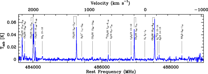
In Fig. 2, the full Herschel-HIFI WBS spectrum is presented. Although the bandwidth of the WBS data is 4 GHz, the entire spectrum covers 5.35 GHz as a result of combining eight different observations where the LO frequencies were slightly shifted in each of the settings. The $rms$ of this spectrum is 1.3 mK in 0.35 km s^-1 bin, therefore many faint lines are detected near the main targeted O₂ 3₃–1₂ line. These lines include some methanol (CH₃OH) lines, together with e.g., SO₂, NH₂D, and D₂CO lines. These lines are shown in Fig. 12 (in the Appendix) in detail, and are tabulated with the observed information in Table 9 (in the Appendix).

3.1 O₂

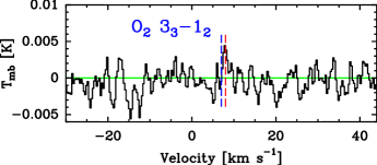
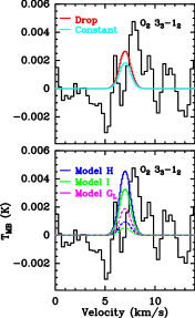
A blow-up of the HIFI spectrum centred around the O₂ $N_{J}$ =3₃–1₂ at 487 GHz position is presented in Fig. 3. The source velocity of IRAS 4A is $V_{\rm LSR}$ =7.0 km s^-1 as determined from many C¹⁸O lines (Yıldız et al. 2012), and is indicated by the blue dashed line in the figure. This spectrum of 7.7 hours integration time staring at the IRAS 4A source position is still not sufficient for a firm detection of the O₂ line at 487 GHz at the source velocity. However, a tentative detection at $V_{\rm LSR}$ =8.0 km s^-1 (red dashed line in Fig. 3) is seen and will be discussed in more detail in Sect. 5.

3.2 NO

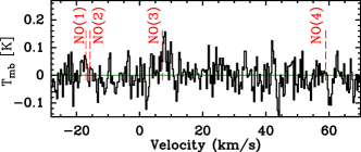
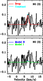
In Fig. 4, the JCMT spectrum covering the hyperfine components of the NO $J$ =5/2–3/2 transitions are presented. For this specific transition, the expected ratios of the line intensities in the optically thin limit are NO (1) : NO (2) : NO (3) : NO (4) = 75:126:200:24. The JCMT observations have an $rms$ of 46 mK in 0.3 km s^-1 bin and 4 $\sigma$ emission is detected only at the intrinsically strongest hyperfine transition, NO (3), with an integrated intensity of 0.18 K km s^-1 centred at $V_{\rm LSR}$ =8.0 km s^-1. No emission is detected for the $V_{\rm LSR}$ =7.0 km s^-1 component, however 3 $\sigma$ upper limit values are provided in Table 1.

3.3 C¹⁸O

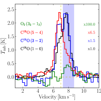
Figure 5 shows the C¹⁸O 1–0, 3–2, and 5–4 lines overplotted on the O₂ line. The peak of the C¹⁸O emission shifts from $V_{\rm LSR}$ =8.0 km s^-1 to 7.0 km s^-1 as $J$ increases. The C¹⁸O 1–0 line is expected to come primarily from the surrounding cloud at 8.0 km s^-1 due to the low energy of the transition ( $E_{\rm up}$ = 5.3 K). On the other hand, the 5–4 line has higher energy ( $E_{\rm up}$ = 79 K), therefore traces the warmer parts of the protostellar envelope at 7.0 km s^-1. As a sanity check, the ¹³CO 1–0, 3–2, and 6–5 transitions from Yıldız et al. (2012) were also inspected and their profiles are consistent with those of the C¹⁸O lines, however they are not included here due to their high opacities. The integrated intensities $\int T_{\rm mb}{\rm d}V$ for each of the 7.0 km s^-1 and 8.0 km s^-1 components are given in Table 1.

3.4 Column densities and abundances

3.4.1 Constant excitation temperature results

Table 3: Summary of column densities in a 44

\arcsec

beam. See text for the conditions used for the calculations.

Molecule	Column Density [cm^-2]		Abundance w.r.t. H₂
	$N$ (7 km s^-1)	$N$ (8 km s^-1)	$X$ (7 km s^-1)	$X$ (8 km s^-1)
O₂	$<$ 1.2 $\times$ 10¹⁵^(a)𝑎(a)^(a)𝑎(a)footnotemark: $(a)$	(2.8–4.3) $\times$ 10¹⁵	$\leq$ 5.7 $\times$ 10^-9	(1.3–2.1) $\times$ 10^-8
C¹⁸O	(3.2–6.1) $\times$ 10¹⁴	(1.8–2.3) $\times$ 10¹⁵	(1.7-3.0) $\times$ 10^-9	(4.3–2.2) $\times$ 10^-7
NO	$<$ 1.9 $\times$ 10¹⁴^(a)𝑎(a)^(a)𝑎(a)footnotemark: $(a)$	2.3 $\times$ 10¹⁴	$\leq$ 9.0 $\times$ 10^-10	2.3 $\times$ 10^-8
H₂	2.1 $\times$ 10²³	1 $\times$ 10²²^(c)𝑐(c)^(c)𝑐(c)footnotemark: $(c)$	…	…

⁶⁶6

A first simple estimate of the O₂ abundance limit in the IRAS 4A protostellar envelope ( $V_{\rm LSR}$ =7.0 km s^-1 component) is obtained by computing column densities within the 44 $\arcsec$ beam. The collisional rate coefficients for the O₂ 3₃–1₂ line give a critical density of $n_{\rm cr}$ =1 $\times$ 10³ cm^-3 for low temperatures (Lique 2010; Goldsmith et al. 2011). The density at the 5000 AU radius corresponding to this beam is found to be 4 $\times$ 10⁵ cm^-3 based on the spherical power-law density model of Kristensen et al. (2012, see also Fig. 6 and below). This value is well above the critical density, implying that the O₂ excitation is thermalized. High densities are independently confirmed by the detection of many high excitation lines from molecules with large dipole moments in this source (e.g., Jørgensen et al. 2005; Maret et al. 2005). The width of the O₂ 3₃–1₂ line is taken to be similar to that of C¹⁸O, $\Delta$ V $\approx$ 1.0 km s^-1. The O₂ line is assumed to be optically thin and a temperature of 30 K is used. The 3 $\sigma$ O₂ column density limit at $V_{\rm LSR}$ =7.0 km s^-1 is then $N$ (O₂)=1.1 $\times$ 10¹⁵ cm^-2 assuming Equations 2 and 3 from Yıldız et al. (2012).

The total H₂ column density of the 7.0 km s^-1 component in the 44 $\arcsec$ beam is computed from the model of Kristensen et al. (2012) through $N_{X,\mathrm{beam}}=\int\int n_{X}(z,b){\rm d}zG(b)2\pi b{\rm d}b/\int G(b)2\pi b{\rm d}b$ , where $b$ is the impact parameter, and $G(b)$ is the beam response function. The resulting value is $N$ (H₂)=2.1 $\times$ 10²³ cm^-2, which is an order of magnitude lower than the pencil-beam H₂ column density of 1.9 $\times$ 10²⁴ cm^-2. Using the 44 $\arcsec$ -averaged H₂ column density implies an abundance limit $X$ (O₂) $\leq$ 5.7 $\times$ 10^-9. This observation therefore provides the lowest limit on the O₂ abundance observed to date. It is $\sim$ 4 orders of magnitude lower than the pure gas phase chemical model predictions of $X$ (O₂) $\sim$ 7 $\times$ 10^-5.

Another option is to compare the O₂ column density directly with that of C¹⁸O. These lines trace the part of the envelope where CO and, by inference, O₂ are not frozen out because of their similar binding energies (Collings et al. 2004; Acharyya et al. 2007). Using the C¹⁸O lines therefore provides an alternative constraint on the models. The C¹⁸O lines are also thermalized, and assuming a temperature of 30 K, its inferred column density is calculated as (3.2–6.1) $\times$ 10¹⁴ cm^-2, depending on the adopted lines. The corresponding abundance ratio is $N$ (O₂)/ $N$ (C¹⁸O)= $\leq$ 3.5 so $N$ (O₂)/ $N$ (CO) $\leq 6.4\times$ 10^-3 assuming CO/C¹⁸O=550.

The critical densities for the NO transitions range from $n_{\rm cr\,NO(1)}$ =2.4 $\times$ 10⁴ cm^-3 to $n_{\rm cr\,NO(4)}$ =7.0 $\times$ 10³ cm^-3), so LTE is again justified. For the 3 $\sigma$ upper limit on the NO (3) line in the 7.0 km s^-1 component, the inferred column density is $N$ (NO)= $<$ 1.9 $\times$ 10¹⁴ cm^-2, assuming $T_{\rm kin}$ =30 K and no beam dilution. Thus, the implied NO abundance is $N$ (NO)/ $N$ (H₂)= $X$ (NO) $\leq$ 9.0 $\times$ 10^-10. All column densities and abundances associated with the protostellar source at $V_{\rm LSR}$ = 7.0 km s^-1 are summarized in Table 6.

3.4.2 Abundance variation models

The above analysis assumes constant physical conditions along the line of sight as well as constant abundances. It is well known from multi-line observations of C¹⁸O that the CO abundance varies throughout the envelope, dropping by more than an order of magnitude in the cold freeze-out zone (e.g., Jørgensen et al. 2002; Yıldız et al. 2010, 2012). 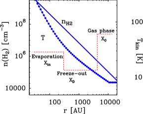A more sophisticated analysis of the O₂ abundance is therefore obtained by using a model of the IRAS 4A envelope in which the density and temperature vary with position. The envelope structure presented in Fig. 6 has been determined by modeling the continuum emission (both the spectral energy distribution and the submillimeter spatial extent) using the 1D spherically symmetric dust radiative transfer code DUSTY (Ivezić & Elitzur 1997). A power-law density profile is assumed with an index $p$ , i.e., $n\propto r^{-p}$ , and the fitting method is described in Schöier et al. (2002) and Jørgensen et al. (2002, 2005), and is further discussed in Kristensen et al. (2012) with the caveats explained. The temperature is calculated as a function of position by solving for the dust radiative transfer through the assumed spherical envelopes, heated internally by the luminosity of the source. The gas temperature is assumed to be equal to the dust temperature. The envelope is defined from the inner radius of 33.5 AU up to the outer radius of 33 000 AU, where the density of the outer radius is 1 $\times$ 10⁴ cm^-3. IRAS 4A is taken to be a standalone source; the possible overlap with IRAS 4B is ignored, but any material at large radii along the line of sight within the beam contributes in both the simulated and observed spectra.

The observed line intensities are used to constrain the molecular abundances in the envelope by assuming a trial abundance structure and computing the non-LTE excitation and line intensities with radiative transfer models for the given envelope structure. For this purpose, the Monte Carlo line radiative transfer program Ratran (Hogerheijde & van der Tak 2000) is employed. The simplest approach assumes a constant O₂ abundance through the envelope. 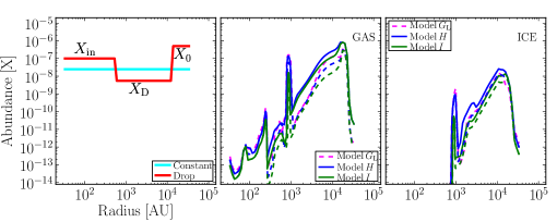Figure 7 (left) shows different abundance profiles, whereas Fig. 8 (top left) shows the resulting line intensities overplotted on the observed O₂ line. The light blue line in Figs. 7 and 8 is the maximum constant O₂ abundance that can be hidden in the noise, which is 2.5 $\times$ 10^-8. This is within a factor of 4 of the simple column density ratio estimate.

A more realistic abundance structure includes a freeze-out zone below 25 K where both O₂ and CO are removed from the gas. Such a CO ‘drop’ abundance profile has been determined for the IRAS 4A envelope via the optically thin C¹⁸O lines from 1–0 to 10–9 in Yıldız et al. (2012). By using the best fit CO abundance structure and assuming a constant O₂/CO abundance ratio, an upper limit of O₂/C¹⁸O $\leq$ 1 is obtained (see red line in Figs. 7 and 8), corresponding to O₂/CO $\leq$ 2 $\times$ 10^-3.

With a 44 $\arcsec$ beam, the 487 GHz line observed with HIFI is mostly sensitive to the bulk of the envelope. Nevertheless, the drop abundance models can be used to estimate the maximum O₂ abundance on smaller scales, to get a firm observational constraint on how much O₂ is in the region where it could enter the embedded circumstellar disk. The radius of such a disk is highly uncertain, but probably on the order of 100 AU (e.g. Visser et al. 2009). According to the drop abundance models, the maximum O₂ abundance that can be “hidden” inside 100 AU is $\sim$ 10^-6. However, the full chemical models from Sect. 4 suggest the actual O₂ abundance on these small scales is several orders of magnitude lower (Fig. 7, middle).

In summary, both the simple column density estimate and the more sophisticated envelope models imply a maximum O₂ abundance of $\sim$ 10^-8, and an O₂/CO ratio of $\leq$ 2 $\times$ 10^-3. For NO, the best fit drop abundance requires NO to be about 8 times lower in abundance than C¹⁸O, to be consistent with our NO non-detection.

4 Gas-grain models for the protostellar envelope

The next step in the analysis is to compare the upper limit for the $V_{\rm LSR}$ =7.0 km s^-1 component with full gas-grain chemical models. The Ohio State University (OSU) gas-grain network (Garrod et al. 2008) is used as the basis for the chemical network, which contains an extensive gas-grain chemistry. There are 590 gas phase and 247 grain surface species and 7500 reactions among them. The subsequent subsections discuss the various chemical processes chemical processes that were considered in the network and are relevant for O₂ and NO are discussed.

4.1 Gas phase O₂ and NO formation

In the gas, O₂ is predominantly formed via reaction (1) between O atoms and OH radicals. The rate coefficient of this reaction has been measured in the temperature range between 39 K and 142 K with the CRESU (Cinetique de Reaction en Ecoulement Supersonique Uniforme) technique by Carty et al. (2006) who found a rate coefficient of 3.5 $\times$ 10^-11 cm³ s^-1 that is constant with temperature. However, several theoretical calculations, especially below 39 K, also exist in the literature. Using quantum mechanical calculations with the so-called $J$ -shifting approximation and neglecting non-adiabatic coupling, Xu et al. (2007) obtained a rate coefficient that decreases as the temperature drops from 100 to 10 K. At 10 K, the computed rate coefficient has fallen to a value of 5.4 $\times$ 10^-13 cm³ s^-1, significantly lower than the 39 K experimental value. However, more recent calculations by Lin et al. (2008), in which the $J$ -shifting approximation has been removed, find a rate coefficient at 10 K of 7.8 $\times$ 10^-12 cm³ s^-1, higher than the Xu et al. (2007) value but still only about 1/4.5 of the experimental value at 39 K. The O₂ formation rates are summarised in Table 7. We have used all three rate coefficients to compare the computed O₂ abundance with the measured upper limit.

Gas-phase NO is predominantly formed through reaction (2). Its gas-phase reaction rate coefficient is listed in Table 7. This reaction is taken from the OSU database and was first determined by Smith et al. (2004).

Table 4: Rate coefficients for O₂ (Equation 1) and NO (Equation 2) formation.

No.	Species	$T$ [K]	Rate coeff. [cm³ s^-1]	References
1.^a𝑎a^a𝑎a $a$ 3 $\sigma$ column density limit.	O₂	39–149	3.5 $\times$ 10^-11	Carty et al. (2006)
2.^b𝑏b^b𝑏b $b$ Beam averaged H₂ column density in a 44 $\arcsec$ beam obtained from the model of Kristensen et al. (2012).	O₂	10	7.8 $\times$ 10^-12	Lin et al. (2008)
3.^c𝑐c^c𝑐c $c$ Computed using the average C¹⁸O column density and abundance ratios of CO/H₂ = 10^-4 and CO/C¹⁸O = 550 (Wilson & Rood 1994).	O₂	10	5.4 $\times$ 10^-13	Xu et al. (2007)
4.	O₂	…	7.5 $\times$ 10^-11 $\times$ (T/300)^-0.25	OSU database
5.	NO	…	7.5 $\times$ 10^-11 $\times$ (T/300)^-0.18	OSU database

⁷⁷7 ^$c$^$c$footnotetext: with

J

-shifting

Table 5: Chemical models considered for the IRAS 4A protostellar envelope

Model	Pre-collapse	Protostellar	O₂ formation rate	$T_{\rm peak}$ (O₂)^a𝑎a^a𝑎a $a$ CRESU measurement	$T_{\rm peak}$ (NO)^a𝑎a^a𝑎a $a$ Ratran model results using a line width of 1.0 km s^-1.
	stage [yr]	stage [yr]	[cm³ s^-1]	[K]	[K]
$A$	5 $\times$ 10⁴	10⁵	7.5 $\times$ 10^-11 $\times$ (T/300)^-0.25	0.119	…
$B$	1 $\times$ 10⁵	10⁵	7.5 $\times$ 10^-11 $\times$ (T/300)^-0.25	0.102	…
$C$	2 $\times$ 10⁵	10⁵	7.5 $\times$ 10^-11 $\times$ (T/300)^-0.25	0.085	…
$D$	3 $\times$ 10⁵	10⁵	7.5 $\times$ 10^-11 $\times$ (T/300)^-0.25	0.073	…
$E$	5 $\times$ 10⁵	10⁵	7.5 $\times$ 10^-11 $\times$ (T/300)^-0.25	0.042	…
$F$	6 $\times$ 10⁵	10⁵	7.5 $\times$ 10^-11 $\times$ (T/300)^-0.25	0.024	…
$G_{\rm O}$	7 $\times$ 10⁵	10⁵	7.5 $\times$ 10^-11 $\times$ (T/300)^-0.25	0.011	…
$G_{\rm L}$ ^b𝑏b^b𝑏b $b$ without $J$ -shifting	7 $\times$ 10⁵	10⁵	7.84 $\times$ 10^-12	0.0019	…
$H_{\rm O}$ ^b𝑏b^b𝑏b $b$ Best fit models. For NO, Case 2 is tabulated.	8 $\times$ 10⁵	10⁵	7.5 $\times$ 10^-11 $\times$ (T/300)^-0.25	0.0046	0.015
$H_{\rm C}$ ^b𝑏b^b𝑏b $b$ Best fit models. For NO, Case 2 is tabulated.	8 $\times$ 10⁵	10⁵	3.50 $\times$ 10^-11	0.0025	…
$H_{\rm L}$ ^b𝑏b^b𝑏b $b$ Best fit models. For NO, Case 2 is tabulated.	8 $\times$ 10⁵	10⁵	7.84 $\times$ 10^-12	0.0010	…
$I_{\rm O}$ ^b𝑏b^b𝑏b $b$ Best fit models. For NO, Case 2 is tabulated.	1 $\times$ 10⁶	10⁵	7.5 $\times$ 10^-11 $\times$ (T/300)^-0.25	0.0033	0.011
$I_{\rm C}$ ^b𝑏b^b𝑏b $b$ Best fit models. For NO, Case 2 is tabulated.	1 $\times$ 10⁶	10⁵	3.50 $\times$ 10^-11	0.0014	…
$I_{\rm L}$ ^b𝑏b^b𝑏b $b$ Best fit models. For NO, Case 2 is tabulated.	1 $\times$ 10⁶	10⁵	7.84 $\times$ 10^-12	0.0005	…
$J$	8 $\times$ 10⁴	2 $\times$ 10⁴	3.50 $\times$ 10^-11	0.106	…
$L$	3 $\times$ 10⁵	10⁵	3.50 $\times$ 10^-11	0.063	…
$M$	3 $\times$ 10⁵	10⁵	7.84 $\times$ 10^-12	0.047	…
$N$	3 $\times$ 10⁵	10⁵	5.40 $\times$ 10^-13	0.018	…
$O$	5 $\times$ 10⁵	10⁵	3.50 $\times$ 10^-11	0.031	…
$P$	5 $\times$ 10⁵	10⁵	7.84 $\times$ 10^-12	0.020	…
$Q$	5 $\times$ 10⁵	10⁵	5.40 $\times$ 10^-13	0.0068	0.091

⁸⁸8 Models

G

H

, and

I

use different rate coefficients for O₂ formation (Eq. 1), as indicated by subscripts: O for OSU, C for Carty et al. (2006), and L for Lin et al. (2008).

4.2 Grain chemistry specific to O₂ and NO

The grain surface chemistry formulation in the OSU code follows the general description by Hasegawa & Herbst (1993) for adsorption, diffusion, reaction, dissociation, and desorption processes, updated and extended by Garrod et al. (2008). The binding energies of various species to the surface are critical parameters in the model. In most of the models, we adopt the binding energies from Garrod & Herbst (2006) appropriate for a water-rich ice surface. However, the possibility of a CO-rich ice surface is also investigated by reducing the binding energies by factors of 0.75 and 0.5, respectively (Bergin et al. 1995; Bergin & Langer 1997).

The presence of O₂ on an interstellar grain can be attributed to two different processes. First, gas-phase O₂ can be accreted on the grain surface during the (pre-)collapse phase and second, atomic oxygen can recombine to form O₂ on the dust grain via the following reaction:

{\rm O+O\rightarrow O_{2}}.

(3)

Following Tielens & Hagen (1982), 800 K is used as the binding (desorption) energy for atomic oxygen on water ice. The binding energy for O₂ on water ice is taken as 1000 K (Cuppen & Herbst 2007), which is an average value obtained from the temperature programmed desorption (TPD) data by Ayotte et al. (2001) and Collings et al. (2004). A ratio of 0.5 between the diffusion barrier and desorption energy has been assumed for the entire calculation (Cuppen & Herbst 2007), so the hopping energy for atomic oxygen is 400 K.

For this hopping energy, one oxygen atom requires 2 $\times$ 10⁵ seconds to hop to another site at 10 K. For comparison, the time needed for a hydrogen atom to hop to another site is around 0.35 seconds, which is a factor of 10⁶ faster. Therefore, instead of forming O₂, an accreted atomic oxygen species will be hydrogenated, leading to the formation of OH and H₂O. It is most unlikely that accreted atomic oxygen produces any significant amount of O₂ on the grain surface during the pre-collapse phase. Recent studies using the continuous time random walk (CTRW) Monte Carlo method do not produce significant O₂ on the grain surface (Cuppen & Herbst 2007). However, elevated grain temperatures ( $\gtrsim$ 20 K), when the residence time of an H atom on the grain is very short and atomic oxygen has enhanced mobility, could be conducive to O₂ formation.

What happens to the O₂ that is formed in the gas phase and accreted onto the dust grains? There are two major destruction pathways. First, the reaction of O₂ with atomic H leads to the formation of HO₂ and H₂O₂, which then could be converted to water following reaction pathways suggested by Ioppolo et al. (2008) and Cuppen et al. (2010):

\rm{O_{2}\buildrel H\over{\longrightarrow}HO_{2}\buildrel H\over{\longrightarrow}H_{2}O_{2}\buildrel H\over{\longrightarrow}H_{2}O+OH.}

(4)

Thus, a longer cold pre-collapse phase would significantly reduce O₂ on the dust grains and turn it into water ice, whereas a shorter pre-collapse phase would yield a higher solid O₂ abundance (Roberts & Herbst 2002). These reactions also depend on the grain temperature: at higher temperatures, the shorter residence time of H atoms on the grain leads to less conversion of O₂.

The second destruction route leads to the formation of ozone through

{\rm O_{2}+O\rightarrow O_{3}.}

(5)

This route is most effective at slightly higher grain temperatures ( $\gtrsim$ 20 K) when atomic oxygen has sufficient mobility to find an O₂ molecule before it gets hydrogenated. Ozone could also be hydrogenated as suggested by Tielens & Hagen (1982) and confirmed in the laboratory by Mokrane et al. (2009) and Romanzin et al. (2010) leading back to O₂:

\rm{O_{3}\buildrel H\over{\longrightarrow}O_{2}+OH.}

(6)

Similarly, accreted NO on the grain surface can undergo various reactions. In particular, recent laboratory experiments have shown that NO is rapidly hydrogenated to NH₂OH at low ice temperatures (Congiu et al. 2012). A critical parameter here is the competition of the different channels for reaction of HNO + H, which can either go back to NO + H₂ or form H₂NO.

The final important ingredient of the gas-grain chemistry is the rate at which molecules are returned from the ice back into the gas phase. Both thermal and non-thermal desorption processes are considered. The first non-thermal process is reactive desorption; here the exothermicity of the reaction is channeled into the desorption of the product with an efficiency determined by a parameter $a_{\rm RRK}$ (Garrod et al. 2007). In these model runs, a value of 0.01 is used, which roughly translates into an efficiency of 1%. Recently, Du et al. (2012) used 7% for the formation of H₂O₂.

Second, there is desorption initiated by UV absorption. Photodissociation of an ice molecule produces two atomic or radical products, which can subsequently recombine and desorb via the reactive desorption mechanism. The photons for this process derive both from the external radiation field and from UV photons generated by ionization of H₂ due to cosmic rays, followed by the excitation of H₂ by secondary electrons. The externally generated UV photons are very effective in diffuse and translucent clouds but their role in dense clouds is limited to the edge of the core (Ruffle & Herbst 2000; Hollenbach et al. 2009). The cosmic-ray-generated internal photons can play an effective role in the dense envelope, with a photon flux of $\approx$ 10⁴ photons cm^-2 s^-1 (Shen et al. 2004). We have considered both sources of radiation in our model. In either case, the rate coefficients for photodissociation on surfaces are assumed to be the same as in the gas phase.

Photodesorption can proceed both by the recombination mechanism described above as well as by kick-out of a neighboring molecule. The combined yields for a variety of species including CO and H₂O have been measured in the laboratory (Öberg et al. 2009a, b; Muñoz Caro et al. 2010) and computed through molecular dynamics simulations for the case of H₂O by Andersson & van Dishoeck (2008) and Arasa et al. (2010). Finally, there is the heating of grains via direct cosmic ray bombardment, which is effective for weakly bound species like CO and O₂ and included following the formulae and parameters of Hasegawa & Herbst (1993).

4.3 Model results

Our physical models have two stages, the “pre-collapse stage” and the “protostellar stage”. In the pre-collapse stage, the hydrogen density is $n_{\rm H}$ =10⁵ cm^-3, visual extinction $A_{\rm V}$ =10 mag, the cosmic-ray ionization parameter, $\zeta$ = 1.3 $\times$ 10¹⁷ s^-1, and the (gas and grain) temperature, $T$ =10 K, which are standard parameters representative of cold cores. The initial elemental abundances of carbon, oxygen and nitrogen are 7.30 $\times$ 10^-5, 1.76 $\times$ 10^-4 and 2.14 $\times$ 10^-5, respectively, in the form of atomic C⁺, O and N. All hydrogen is assumed to be in molecular form initially. In the second stage, the output abundance of the first phase is used as the initial abundance at each radial distance with the density, temperature and visual extinction parameters at each radius taken from the IRAS 4A model shown in Fig. 6. We assume that the transition to the protostellar phase from the pre-collapse stage is instantaneous i.e., the power-law density and temperature structure are established quickly, consistent with evolutionary models (Lee et al. 2004; Young & Evans 2005).

To explain the observed spectra of O₂, both the pre-collapse time and protostellar time as well as the O₂ formation rates are varied. Analysis of CO and HCO⁺ multi-line observations in pre- and protostellar sources have shown that the high density pre-collapse stage typically lasts a few $\times$ 10⁵ yr (e.g., Jørgensen et al. 2005; Ward-Thompson et al. 2007). The models $A$ to $Q$ have different parameters and timescales which are listed in Table 8. Those models result in abundance profiles in the envelope at each time step and radius. These profiles are then run in Ratran in order to compare directly with the observations.

Figure 7 (middle) shows examples of model abundance profiles. All model runs predict lower O₂ abundances than the evolutionary models of Visser et al. (2011), whose chemical network did not include any grain-surface processing of O₂. The line emission from our models is compared to the observations in Fig. 8 (bottom left). Table 8 summarizes the resulting O₂ peak temperatures for each of the models. All models except $H$ and $I$ overproduce the observed O₂ emission of at most a few mK, by up to two orders of magnitude in the peak temperature. The models that are consistent with the data have in common longer pre-collapse stages; in particular Model $I$ , which has the longest pre-collapse stage of 10⁶ years, best fits the 3 $\sigma$ O₂ limit. Using a lower rate coefficient for the O+OH reaction of 7.84 $\times$ 10^-12 cm³ s^-1 (Lin et al. 2008) for the same best fit models ( $H_{\rm L}$ and $I_{\rm L}$ ) results in a factor of 5 lower emission. In this case, the pre-collapse stage can be shortened to $\sim$ 7 $\times$ 10⁵ yr (Model $G_{\rm L}$ ).

For NO, the $H$ and $I$ models were calculated twice. In Case 1, hydrogenation of HNO leads back to NO and H₂ and in Case 2 hydrogenation of HNO leads to H₂NO as suggested by Congiu et al. (2012). Comparison of the results from Case 1 with observations shows significant overproduction of the observed NO emission, whereas Case 2 is consistent with an upper limit of 0.05 K (1 $\sigma$ ). Therefore, a combination of both reactions appears to be needed.

These results for IRAS 4A suggest that a long pre-collapse stage is characteristic of the earliest stages of star formation, in which atomic and molecular oxygen are frozen-out onto the dust grains and converted into water ice, as proposed by Bergin et al. (2000). Similarly, the rapid conversion of NO to other species on the grains limits its gas-phase abundance. It is clear that the grain surface processes are much more important than those of the pure gas-phase chemistry in explaining the O₂ and NO observations. The timescale for NGC 1333 IRAS 4A is at the long end of that inferred more generally from observations.

The model results show that the fraction of O₂ in the gas and left on the grains must indeed be very small, dropping to $\leq$ 10^-9 close to the protostar (Fig. 7, right). This in turn implies that the gas and ice that enter the disk are very poor in O₂. Although IRAS 4A is the only low-mass protostar that has been observed to this depth, the conclusions drawn for IRAS 4A probably hold more generally. Thus, unless there is significant production of O₂ in the disk, the icy planetesimals will also be poor in O₂.

5 Tentative detection of O₂ in the 8 km s^-1 cloud

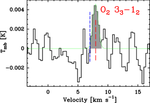
Although there is no sign of O₂ emission at the velocity of the dense protostellar envelope (7.0 km s^-1), a 4.5 $\sigma$ tentative detection of O₂ 3₃–1₂ line emission is found at $V_{\rm LSR}$ =8.0 km s^-1, the velocity of the more extended NGC 1333 molecular cloud (Fig. 9; Loren 1976; Liseau et al. 1988). The feature is also seen in individual H and V polarization spectra. The peak intensity of the tentative detection is $T_{\rm mb}$ =4.6 mK, the line width $\Delta V$ =1.3 km s^-1, and the integrated intensity is $\int T_{\rm mb}{\rm d}V$ =6.9 mK km s^-1 between the velocities of 6.5 to 9.7 km s^-1. The large HIFI beam size of 44 $\arcsec$ encompasses both the extended cloud as well as the compact envelope. Since any O₂ emission is optically thin, the two components cannot block each other, even if slightly overlapping in velocity.

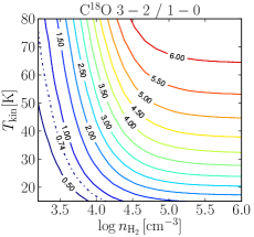
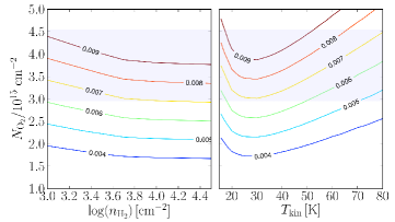
The density in the surrounding cloud at 8.0 km s^-1 is expected to be significantly lower than that in the envelope. Figure 13 (in the Appendix) presents the C¹⁸O 3–2/1–0 ratio for the 8.0 km s^-1 component. The observed value is consistent with a wide range of kinetic temperatures from 20 K to 70 K, with corresponding densities in a narrow range from 7 $\times$ 10³ to 2 $\times$ 10³ cm^-3, respectively. C¹⁸O column densities from the 3–2 and 1–0 line intensities are then (2.3–1.8) $\times$ 10¹⁵ cm^-2 for this range of physical parameters.

For the same range of conditions, the O₂ column density is (2.8–4.3) $\times$ 10¹⁵ cm^-2 (Fig. 10). The inferred abundance ratios are $N$ (O₂)/ $N$ (C¹⁸O)=1.2 to 2.4, and $N$ (O₂)/ $N$ (CO)=(2.2–4.3) $\times$ 10^-3. Assuming CO/H₂ $\approx$ 10^-4 gives $N$ (O₂)/ $N$ (H₂)=(2.2–4.3) $\times$ 10^-7. Interestingly, the inferred O₂ abundance is in between the values found for the Orion and $\rho$ Oph A clouds (Goldsmith et al. 2011; Liseau et al. 2012). By assuming $T_{\rm kin}$ =30 K, the implied NO column density is 2.3 $\times$ 10¹⁴ cm^-2, leading to $N$ (NO)/ $N$ (O₂)=(5.3–8.1) $\times$ 10^-2 and $N$ (NO)/ $N$ (H₂)=2.3 $\times$ 10^-8.

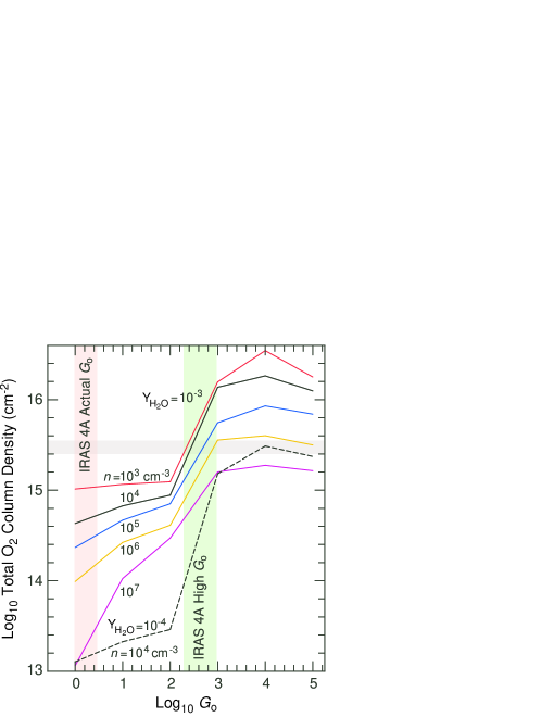
Can such an O₂ column density and abundance be reproduced by chemical models? For the surrounding cloud, a large gas-grain model is not needed. Instead, the PDR models of Hollenbach et al. (2009), which include a simplified gas-grain chemistry, are adequate to model the emission. Figure 11 is a plot adapted from Melnick et al. (2012), which shows the values of interstellar radiation field $G_{0}$ required to reproduce the range of O₂ column densities according to the model described in Hollenbach et al. (2009). The horizontal grey band bounds the total observed O₂ column density range of (2.8–4.3) $\times$ 10¹⁵ cm^-2, while the vertical green band shows the range of $G_{0}$ values required to produce this range of O₂ column densities for gas densities between 10³ cm^-3 and 10⁷ cm^-3. For our low inferred densities of ¡10⁴ cm^-3, a high $G_{0}$ value of 300–650 fits the data. There is no external source in the NGC 1333 region which can provide this level of UV illumination, not even the nearby B8 V type star BD+30 $\degr$ 549 ( $\alpha$ = $3^{\mathrm{h}}29^{\mathrm{m}}19\aas@@fstack{s}78$ , $\delta$ = $+31\degr 24\arcmin 57\aas@@fstack{\prime\prime}05$ (J2000); $\sim$ 0.8 pc away; van Leeuwen 2007). The $G_{0}$ value from this star at our position is at most 2.8 and can therefore not explain the high- $G_{0}$ scenario. Models with a slightly higher (factor of 2) water ice photodesorption yield than the standard value of $Y_{\rm H_{2}O}$ =10^-3 would fit better the low- $G_{0}$ regime, where the value of $G_{0}$ is between the interstellar value of 1 and 2.8. This value of $Y_{\rm H_{2}O}$ is within the uncertainties of the laboratory (Öberg et al. 2009a) and theoretical work (Arasa et al. 2010). More generally, a factor of two uncertainty in abundance can readily result from the combined uncertainties of the individual rate coefficients that lead to O₂ formation and destruction (Wakelam et al. 2006), so it does not necessarily imply an increased value of $Y_{\rm H_{2}O}$ . Considering the uncertainties in rate coefficients as well as possible increase in $Y$ , there does not seem to be a problem having the actual low value of $G_{0}$ produce the observed column density of molecular oxygen.

6 Conclusions

We have presented the first deep (7.7 hr) Herschel-HIFI observations of the O₂ 3₃–1₂ line at 487 GHz towards a deeply embedded Class 0 protostar, NGC 1333 IRAS 4A. The results from the observations and models can be summarized as follows.

•

No O₂ emission is detected from the protostellar envelope, down to a 3 $\sigma$ upper limit of $X$ (O₂) $\lesssim$ 6 $\times$ 10^-9, the lowest O₂ abundance limit toward a protostar to date. The O₂/CO limit is $\leq$ 6 $\times$ 10^-3.
•

A full gas-grain chemical model coupled with the physical structure of the envelope is compared to our data consisting of two stages, a “pre-collapse stage” and “protostellar stage”. Best fits to the observed upper limit on the O₂ line suggest a long pre-collapse stage ( $\sim$ 0.7–1 $\times$ 10⁶ years), during which atomic oxygen is frozen out onto the dust grains and converted into water ice. Also, at least a fraction of NO must be converted to more complex nitrogen species in the ice.
•

The low O₂ abundance in the gas and on the grains in the inner envelope implies that the material entering the disk is very poor in O₂.
•

A 4.5 $\sigma$ tentative O₂ detection is found at $V_{\rm LSR}$ = 8.0 km s^-1, which is interpreted as emission originating from the surrounding more extended NGC 1333 cloud. At this velocity, also a weak NO line is seen.
•

Comparison with PDR models of Hollenbach et al. (2009) suggests a high $G_{0}$ of 300–650 in the surrounding cloud for the low inferred density of ¡10⁴ cm^-3. For the low $G_{0}$ inferred at our position, either the H₂O ice photodesorption yield would need to be increased by a factor of $\sim$ 2 or combination of other minor changes in reaction rates would be needed to reproduce the observed $N$ (O₂) with a reasonable value of $G_{0}$ .

Acknowledgements.

UAY and astrochemistry in Leiden are supported by the Netherlands Research School for Astronomy (NOVA), by a Spinoza grant and grant 614.001.008 from the Netherlands Organisation for Scientific Research (NWO), and by the European Community’s Seventh Framework Programme FP7/2007-2013 under grant agreement 238258 (LASSIE) and 291141 (CHEMPLAN). This work was carried out in part at the Jet Propulsion Laboratory, which is operated by the California Institute of Technology under contract with NASA. The authors are grateful to many funding agencies and the HIFI-ICC staff, who has been contributing for the construction of Herschel and HIFI for many years. HIFI has been designed and built by a consortium of institutes and university departments from across Europe, Canada and the United States under the leadership of SRON Netherlands Institute for Space Research, Groningen, The Netherlands and with major contributions from Germany, France and the US. Consortium members are: Canada: CSA, U.Waterloo; France: CESR, LAB, LERMA, IRAM; Germany: KOSMA, MPIfR, MPS; Ireland, NUI Maynooth; Italy: ASI, IFSI-INAF, Osservatorio Astrofisico di Arcetri- INAF; Netherlands: SRON, TUD; Poland: CAMK, CBK; Spain: Observatorio Astronómico Nacional (IGN), Centro de Astrobiología (CSIC-INTA). Sweden: Chalmers University of Technology - MC2, RSS

\&

GARD; Onsala Space Observatory; Swedish National Space Board, Stockholm University - Stockholm Observatory; Switzerland: ETH Zurich, FHNW; USA: Caltech, NASA/JPL, NHSC.

References

Acharyya et al. (2007) Acharyya, K., Fuchs, G. W., Fraser, H. J., van Dishoeck, E. F., & Linnartz, H. 2007, A&A, 466, 1005
Andersson & van Dishoeck (2008) Andersson, S. & van Dishoeck, E. F. 2008, A&A, 491, 907
André & Montmerle (1994) André, P. & Montmerle, T. 1994, ApJ, 420, 837
Arasa et al. (2010) Arasa, C., Andersson, S., Cuppen, H. M., van Dishoeck, E. F., & Kroes, G.-J. 2010, J. Chem. Phys., 132, 184510
Ayotte et al. (2001) Ayotte, P., Scott, S. R., Stevenson, K. P., et al. 2001, J. Geophys. Res., 106, 33387
Bergin & Langer (1997) Bergin, E. A. & Langer, W. D. 1997, ApJ, 486, 316
Bergin et al. (1995) Bergin, E. A., Langer, W. D., & Goldsmith, P. F. 1995, ApJ, 441, 222
Bergin et al. (2000) Bergin, E. A., Melnick, G. J., Stauffer, J. R., et al. 2000, ApJ, 539, L129
Black & Smith (1984) Black, J. H. & Smith, P. L. 1984, ApJ, 277, 562
Blake et al. (1995) Blake, G. A., Sandell, G., van Dishoeck, E. F., et al. 1995, ApJ, 441, 689
Bottinelli et al. (2007) Bottinelli, S., Ceccarelli, C., Williams, J. P., & Lefloch, B. 2007, A&A, 463, 601
Carty et al. (2006) Carty, D., Goddard, A., Kohler, S., Sims, I., & Smith, I. 2006, J. Phys. Chem. A, 110, 3101
Collings et al. (2004) Collings, M. P., Anderson, M. A., Chen, R., et al. 2004, MNRAS, 354, 1133
Congiu et al. (2012) Congiu, E., Fedoseev, G., Ioppolo, S., et al. 2012, ApJ, 750, L12
Cuppen & Herbst (2007) Cuppen, H. M. & Herbst, E. 2007, ApJ, 668, 294
Cuppen et al. (2010) Cuppen, H. M., Ioppolo, S., Romanzin, C., & Linnartz, H. 2010, Phys. Chem. Chem. Phys., 12, 12077
Curtis et al. (2010) Curtis, E. I., Richer, J. S., & Buckle, J. V. 2010, MNRAS, 401, 455
de Graauw et al. (2010) de Graauw, T., Helmich, F. P., Phillips, T. G., et al. 2010, A&A, 518, L6
Doty et al. (2004) Doty, S. D., Schöier, F. L., & van Dishoeck, E. F. 2004, A&A, 418, 1021
Drouin et al. (2010) Drouin, B. J., Yu, S., Miller, C. E., et al. 2010, J. Quant. Spectrosc. Rad. Trans., 111, 1167
Du et al. (2012) Du, F., Parise, B., & Bergman, P. 2012, A&A, 538, A91
Garrod & Herbst (2006) Garrod, R. T. & Herbst, E. 2006, A&A, 457, 927
Garrod et al. (2007) Garrod, R. T., Wakelam, V., & Herbst, E. 2007, A&A, 467, 1103
Garrod et al. (2008) Garrod, R. T., Weaver, S. L. W., & Herbst, E. 2008, ApJ, 682, 283
Goldsmith et al. (2011) Goldsmith, P. F., Liseau, R., Bell, T. A., et al. 2011, ApJ, 737, 96
Goldsmith et al. (2000) Goldsmith, P. F., Melnick, G. J., Bergin, E. A., et al. 2000, ApJ, 539, L123
Goldsmith et al. (1985) Goldsmith, P. F., Snell, R. L., Erickson, N. R., et al. 1985, ApJ, 289, 613
Gutermuth et al. (2008) Gutermuth, R. A., Myers, P. C., Megeath, S. T., et al. 2008, ApJ, 674, 336
Hasegawa & Herbst (1993) Hasegawa, T. I. & Herbst, E. 1993, MNRAS, 261, 83
Herbst & Klemperer (1973) Herbst, E. & Klemperer, W. 1973, ApJ, 185, 505
Hirota et al. (2008) Hirota, T., Bushimata, T., Choi, Y. K., et al. 2008, PASJ, 60, 37
Hogerheijde & van der Tak (2000) Hogerheijde, M. R. & van der Tak, F. F. S. 2000, A&A, 362, 697
Hollenbach et al. (2009) Hollenbach, D., Kaufman, M. J., Bergin, E. A., & Melnick, G. J. 2009, ApJ, 690, 1497
Ioppolo et al. (2008) Ioppolo, S., Cuppen, H. M., Romanzin, C., van Dishoeck, E. F., & Linnartz, H. 2008, ApJ, 686, 1474
Ivezić & Elitzur (1997) Ivezić, Z. & Elitzur, M. 1997, MNRAS, 287, 799
Jørgensen et al. (2002) Jørgensen, J. K., Schöier, F. L., & van Dishoeck, E. F. 2002, A&A, 389, 908
Jørgensen et al. (2005) Jørgensen, J. K., Schöier, F. L., & van Dishoeck, E. F. 2005, A&A, 437, 501
Jørgensen et al. (2009) Jørgensen, J. K., van Dishoeck, E. F., Visser, R., et al. 2009, A&A, 507, 861
Kristensen et al. (2012) Kristensen, L. E., van Dishoeck, E. F., Bergin, E. A., et al. 2012, A&A, 542, A8
Kristensen et al. (2010) Kristensen, L. E., Visser, R., van Dishoeck, E. F., et al. 2010, A&A, 521, L30
Kutner & Ulich (1981) Kutner, M. L. & Ulich, B. L. 1981, ApJ, 250, 341
Larsson et al. (2007) Larsson, B., Liseau, R., Pagani, L., et al. 2007, A&A, 466, 999
Lee et al. (2004) Lee, J.-E., Bergin, E. A., & Evans, II, N. J. 2004, ApJ, 617, 360
Lefloch et al. (1998) Lefloch, B., Castets, A., Cernicharo, J., & Loinard, L. 1998, ApJ, 504, L109
Lin et al. (2008) Lin, S. Y., Guo, H., Honvault, P., Xu, C., & Xie, D. 2008, J. Chem. Phys., 128
Lique (2010) Lique, F. 2010, J. Chem. Phys., 132, 044311
Liseau et al. (2012) Liseau, R., Goldsmith, P. F., Larsson, B., et al. 2012, A&A, 541, A73
Liseau et al. (1988) Liseau, R., Sandell, G., & Knee, L. B. G. 1988, A&A, 192, 153
Loren (1976) Loren, R. B. 1976, ApJ, 209, 466
Maret et al. (2005) Maret, S., Ceccarelli, C., Tielens, A. G. G. M., et al. 2005, A&A, 442, 527
Melnick et al. (2000) Melnick, G. J., Stauffer, J. R., Ashby, M. L. N., et al. 2000, ApJ, 539, L77
Melnick et al. (2012) Melnick, G. J., Tolls, V., Goldsmith, P. F., et al. 2012, ApJ, 752, 26
Mokrane et al. (2009) Mokrane, H., Chaabouni, H., Accolla, M., et al. 2009, ApJ, 705, L195
Muñoz Caro et al. (2010) Muñoz Caro, G. M., Jiménez-Escobar, A., Martín-Gago, J. Á., et al. 2010, A&A, 522, A108
Müller et al. (2005) Müller, H. S. P., Schlöder, F., Stutzki, J., & Winnewisser, G. 2005, Journal of Molecular Structure, 742, 215
Nordh et al. (2003) Nordh, H. L., von Schéele, F., Frisk, U., et al. 2003, A&A, 402, L21
Öberg et al. (2009a) Öberg, K. I., Linnartz, H., Visser, R., & van Dishoeck, E. F. 2009a, ApJ, 693, 1209
Öberg et al. (2009b) Öberg, K. I., van Dishoeck, E. F., & Linnartz, H. 2009b, A&A, 496, 281
Ott (2010) Ott, S. 2010, in Astronomical Society of the Pacific Conference Series, Vol. 434, Astronomical Data Analysis Software and Systems XIX, ed. Y. Mizumoto, K.-I. Morita, & M. Ohishi, 139
Pagani et al. (1993) Pagani, L., Langer, W. D., & Castets, A. 1993, A&A, 274, L13
Pagani et al. (2003) Pagani, L., Olofsson, A. O. H., Bergman, P., et al. 2003, A&A, 402, L77
Pickett et al. (2010) Pickett, H. M., Poynter, R. L., Cohen, E. A., et al. 2010, Journal of Quantitative Spectroscopy & Radiative Transfer, 111, 1617
Pilbratt et al. (2010) Pilbratt, G. L., Riedinger, J. R., Passvogel, T., et al. 2010, A&A, 518, L1
Roberts & Herbst (2002) Roberts, H. & Herbst, E. 2002, A&A, 395, 233
Roelfsema et al. (2012) Roelfsema, P. R., Helmich, F. P., Teyssier, D., et al. 2012, A&A, 537, A17
Romanzin et al. (2010) Romanzin, C., Arzoumanian, E., Es-Sebbar, E., et al. 2010, Planet. Space Sci., 58, 1748
Ruffle & Herbst (2000) Ruffle, D. P. & Herbst, E. 2000, MNRAS, 319, 837
Schöier et al. (2002) Schöier, F. L., Jørgensen, J. K., van Dishoeck, E. F., & Blake, G. A. 2002, A&A, 390, 1001
Schöier et al. (2005) Schöier, F. L., van der Tak, F. F. S., van Dishoeck, E. F., & Black, J. H. 2005, A&A, 432, 369
Shen et al. (2004) Shen, C. J., Greenberg, J. M., Schutte, W. A., & van Dishoeck, E. F. 2004, A&A, 415, 203
Smith et al. (2004) Smith, I. W. M., Herbst, E., & Chang, Q. 2004, MNRAS, 350, 323
Tielens & Hagen (1982) Tielens, A. G. G. M. & Hagen, W. 1982, A&A, 114, 245
Černis (1990) Černis, K. 1990, Ap&SS, 166, 315
van der Tak et al. (2007) van der Tak, F. F. S., Black, J. H., Schöier, F. L., Jansen, D. J., & van Dishoeck, E. F. 2007, A&A, 468, 627
van Dishoeck et al. (2011) van Dishoeck, E. F., Kristensen, L. E., Benz, A. O., et al. 2011, PASP, 123, 138
van Leeuwen (2007) van Leeuwen, F. 2007, A&A, 474, 653
Visser et al. (2011) Visser, R., Doty, S. D., & van Dishoeck, E. F. 2011, A&A, 534, A132
Visser et al. (2009) Visser, R., van Dishoeck, E. F., Doty, S. D., & Dullemond, C. P. 2009, A&A, 495, 881
Wakelam et al. (2006) Wakelam, V., Herbst, E., Selsis, F., & Massacrier, G. 2006, A&A, 459, 813
Ward-Thompson et al. (2007) Ward-Thompson, D., André, P., Crutcher, R., et al. 2007, Protostars and Planets V, 33
Wilson & Rood (1994) Wilson, T. L. & Rood, R. 1994, ARA&A, 32, 191
Woodall et al. (2007) Woodall, J., Agúndez, M., Markwick-Kemper, A. J., & Millar, T. J. 2007, A&A, 466, 1197
Xu et al. (2007) Xu, C., Xie, D., Honvault, P., Lin, S. Y., & Guo, H. 2007, Journal of Chemical Physics, 127
Yıldız et al. (2012) Yıldız, U. A., Kristensen, L. E., van Dishoeck, E. F., et al. 2012, A&A, 542, A86
Yıldız et al. (2010) Yıldız, U. A., van Dishoeck, E. F., Kristensen, L. E., et al. 2010, A&A, 521, L40
Young & Evans (2005) Young, C. H. & Evans, II, N. J. 2005, ApJ, 627, 293

Appendix A HIFI O₂ Spectrum

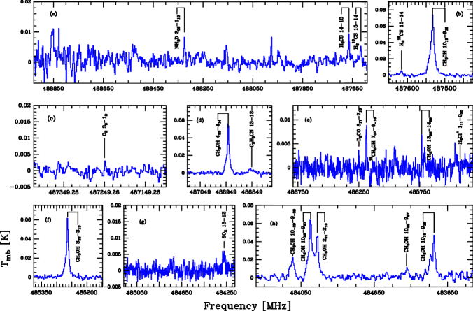
Table 6: Overview of the other lines observed in the same spectrum. The level energies, Einstein A coefficients, and line frequencies are from the LAMDA, JPL and CDMS databases (Schöier et al. 2005; Pickett et al. 2010; Müller et al. 2005).

Mol.	Trans.	$E_{\mathrm{u}}/k_{\mathrm{B}}$	$A_{\rm ul}$	Frequency	$\int T_{\mathrm{MB}}\mathrm{d}V$	$T_{\mathrm{peak}}$	FWHM
	$J_{\mathrm{u}}$ - $J_{\mathrm{l}}$	[K]	[s^-1]	[GHz]	[mK km s^-1]	[mK]	[km s^-1]
NH₂D	2₀₂–1₁₀	47.2	1.36 $\times$ 10^-4	488.323810	25	10	3.4
H₂CS	14–13	188.8	1.76 $\times$ 10^-3	487.663321	28	9	3.3
H ${}_{2}^{13}$ CS	15–14	200.5	1.77 $\times$ 10^-3	487.615288	22	5	3.9
CH₃OH	10₁₉–9₁₈	143.3	5.15 $\times$ 10^-4	487.531887	580	80	8.2
O₂	3₃–1₂	26.38	8.66 $\times$ 10^-9	487.249264	7	…	…
CH₃OH	4₂₃–4₁₄	60.9	5.45 $\times$ 10^-4	486.940837	390	60	7.2
C₂H₅CN	13–12	66.9	1.00 $\times$ 10^-6	486.849912	36	5	7.3
D₂CO	8₁₇–7₁₆	111.0	3.36 $\times$ 10^-3	486.248662	9	7	1.1
¹³CH₃OH	7₀₇–6₁₆	76.5	3.02 $\times$ 10^-4	486.188242	39	10	3.9
CH₃OH	13₆₈–14₅₉	404.8	1.16 $\times$ 10^-4	485.732280	12	10	1.4
H₂Cl⁺	1₁₁–0₀₀	…	…	485.420796	$-$ 5	$-$ 6	0.8
CH₃OH	3₂₂–3₁₃	51.6	5.02 $\times$ 10^-4	485.263263	401	71	7.3
SO₂	13–12	105.8	5.42 $\times$ 10^-4	484.270879	26	6	1.1
CH₃OH	10_-29–9_-28	153.6	4.88 $\times$ 10^-4	484.071775	170	20	8.4
CH₃OH	10₂₈–9₂₇	150.0	4.83 $\times$ 10^-4	484.023168	490	70	8.2
CH₃OH	2₂₁–2₁₂	44.7	3.99 $\times$ 10^-4	484.004740	280	50	4.9
CH₃OH	10₂₈–9₂₇	165.4	4.90 $\times$ 10^-4	483.761387	70	10	5.8
CH₃OH	10₁₉–9₁₈	148.7	5.13 $\times$ 10^-4	483.686308	210	50	4.2

⁹⁹9

rms

is 1.3 mK and in 0.35 km s^-1 bin. Identifications refer to the 7.0 km s^-1 component.

Appendix B RADEX Calculations for C¹⁸O

The integrated intensity ratio of C¹⁸O 3–2/1–0 is equal to 0.74 for the 8.0 km s^-1 component. This ratio can be analysed using the RADEX non-LTE excitation and radiative transfer program (van der Tak et al. 2007) to constrain the physical parameters. Figure 13 presents the integrated intensity ratios as function of temperature and density, obtained for optically thin conditions. The observed ratio is indicated in dash-dotted lines.

Deep observations of O2 toward a low-mass protostar with Herschel-HIFI††thanks: Herschel is an ESA space observatory with science instruments provided by European-led Principal Investigator consortia and with important participation from NASA.