Detecting chaos in a complex system

Abstract

The sequences, given by a 7D map have been analysed by means of the methods, widely used to detect chaos in the real world in order to test their sensitivity to chaotic features of a non-linear system determined by comparatively high number of parameters. The same diagnostic approaches have been applied to the 3D Lorenz map for comparison. The results show that for some of the sequences yielded from the 7D map, the adopted methods were not able to give as straightforward answer to the question if the system is chaotic as in the 3D case. Since the sequences, subject of the analysis, were not contaminated by noise and were sufficiently long, it could be assumed that such difficulties have arisen likely due to specific internal features of the more complex system. It was found also that an increase from 0.01 to 0.5 of the sampling step determining the sequences obtained from the 7D map, masks the chaos in some of them.

1 Introduction

Very often, the decision about chaotic origin of a time series turns out to be a fundamental issue for the study of the processes in the real world (Lorenz, 1991; Marzocchi et al., 1997; Lai et al., 2002; Voss et al., 2009). Such a judgement is usually made basing on the assessment of the attractor invariants – Housdorff dimension and Lyapunov exponents (Marzocchi et al., 1997; Lai et al., 2002; Grassberger et al., 1991; Kodba et al., 2005). Their correct estimation provides important information about the complexity of the system and its dynamics that helps us to create an adequate model of the phenomenon under study.

The reliability of the methods, developed for detecting chaos in the real systems is usually tested on time series yielded from well studied maps. A similar test has been performed here by applying the adopted methods to the sequences obtained from a 7-dimensional (7D) map, defined by 7 parameters, all connected through nonlinear relationships. Such a map was assumed to imitate a comparatively more complex system and, in order to highlight eventual its specific features, the same test has been done with the sequences given by a 3D map. Except for the invariants, the minimal dimension of the space, embedding the reconstructed attractor has been also evaluated, since this parameter gives the number of variables composing the system that is also an important characteristic.

To study the sensitivity of the methods that compute the invariants, the researchers usually take one component of a map assuming that the others should represent the same behaviour (Lorenz, 1991; Grassberger and Procaccia, 1984; Zeng et al., 1991). In the present study, these methods have been applied to each of the sequences, yielded from both 3D and 7D maps. Such a performance was adopted in order to check if each of the sequences generated by the 7D map is able to depicter adequately the system attractor. It was assumed also that the sampling step determining the sequences under study is able to influence the topological properties of the reconstructed attractor and hence, the assessment of the parameters chosen to characterise the system. To analyse such an assumption the evaluations of the corresponding parameters were made by varying the sampling steps of the sequences under study.

2 Methods of nonlinear time series analysis used in the present study

A starting point for the analysis of a nonlinear system presented by a time series is the reconstruction of the embedding phase space and the attractor. Furthermore, an assessment of the Hausdorff dimension $D_{0}$ approximated by estimators allowing easy computation and Lyapunov exponents $\lambda_{l}\,(l=1,2,..,m)$ is usually performed. Next subsections briefly present some widely used algorithms for estimation of these parameters, which have been applied in the present analysis.

2.1 Reconstruction of the system attractor

The reconstruction of the attractor using only one scalar projection (Packard et al., 1980; Takens, 1981) gave a powerful instrument to study the natural phenomena. For a sequence $(x_{i})_{i=1,\,2,\,..,\,N}$ determined by measuring of the variable $x$ at uniquely sampled times $(t_{i})_{i=1,\,2,\,..,\,N}$ the Takens’s theorem (Takens, 1981) affirms that the $m-$component vectors constructed as

$$\mathbf{X}_{i}=(x_{i},\,x_{i+\tau},\,x_{i+2\tau},...,\,x_{i+(m-1)\tau})\,,$$ (1)

where $\tau$ is the so-called time delay, expressed in sampling steps $\Delta t=t_{i+1}-t_{i}$, determine a manifold that realistically represents the attractor of the system, which generates the time series $(x_{i})$. It should be pointed out that there is no a unique optimal choice of the time delay $\tau$ (Grassberger et al., 1991; Zeng et al., 1992a). In the present study the parameter $\tau$ is taken to be the time for which the autocorrelation function drops to $e^{-1}$ or to about 0.37.

2.2 Minimum dimension of the reconstructed embedding space

According to Kennel et al. (1992) an acceptable minimum embedding dimension $m_{K}$ of the attractor can be assessed by looking at the behaviour of the nearest neighbor $\mathbf{X}^{(b)}$ of each vector $\mathbf{X}_{i}$ when the embedding dimension $m$ increases. Assuming Euclidean metric in the phase space the authors found that each $\mathbf{X}^{(b)}$ can be considered as a false nearest neighbor if either of the following two conditions:

$$\frac{|x_{i+m\tau}-x_{i+m\tau}^{(b)}|}{\|\mathbf{X}_{i}-\mathbf{X}^{(b)}\|_{(m)}^{(E)}}>R_{tol}$$ (2)

and

$$\frac{\|\mathbf{X}_{i}-\mathbf{X}^{(b)}\|_{(m+1)}^{(\text{E})}}{R_{A}}>A_{tol}\,,$$ (3)

is held. The expression $\|\mathbf{X}_{i}-\mathbf{X}^{(b)}\|_{(m)}^{(\text{E})}=\sqrt{\sum_{k=1}^{m}\bigl{(}x_{i+(k-1)\tau}-x^{(b)}_{i+(k-1)\tau}\bigr{)}^{2}}$ denotes the Euclidean distance between two vectors in $m-$dimensional embedding spaces and according to Kennel et al. (1992) $R_{tol}$ can be considered higher than 10 and $A_{tol}=2$. The parameter $R_{A}$ represents the size of the attractor and was taken to be equal to the standard deviation of $(x_{i})_{i=1,\,2,\,..,\,N}$. Kennel et al. (1992) assumed that the minimum dimension of the embedding space $m_{K}$ for which the false nearest neighbors percentage (FNNP) drops to a value below 1%, allows unfolding of the attractor. Studding the 3D Lorenz system they found also that for a noise free sequence the FNNP remains lower than 1% for $m>m_{K}=3$, while a noise contaminated time series shows a different behaviour. For low level of the noise the approach gave $m_{K}=4$, whereas for higher level FNNP falls to a value slightly exceeding 1% at $m=m_{K}$ and plateaus for higher embedding dimension. In presence of strong noise the length of such a plateau narrows to a few successive values of $m$ and after that FNNP increases. In case of sequence presenting a stochastic process FNNP drops to a comparatively high value ($>20\%$) and after that rapidly increases.

2.3 Correlation dimension of the attractor

Correlation dimension $D_{2}$ of the attractor, which is a widely used estimator of the Hausdorff dimension $D_{0}$, can be assessed by calculating the correlation integral $C_{m}(\rho)$:

$$C_{m}(\rho)\,=\,\lim_{N\to\infty}\frac{2}{(N+1-W)(N-W)}\times$$

$$\times\sum_{j=W}^{N}\sum_{i=1}^{N-j}\theta(\rho-\|\mathbf{X}_{i}-\mathbf{X}_{i+j}\|^{(\text{Ch})}_{(m)})\,,$$ (4)

where $\theta(\xi)$ is the Heaviside function $\bigl{(}\theta(\xi<0)=0$ and $\theta(\xi\geq 0)=1\bigr{)}$ and $\|\mathbf{X}_{p}-\mathbf{X}_{q}\|^{(\text{Ch})}_{(m)}=\underset{1\leq k\leq m}{\max}\,\bigl{\{}|x_{p+(k-1)\tau}-x_{q+(k-1)\tau}|\bigr{\}}$ is the distance between two vectors in $m$-dimensional embedding space determined here by the Chebishev metric. The correlation integral $C_{m}(\rho)$ was defined by Grassberger and Procaccia (1983) as Eq (2.3) gives it for $W=1$ and later, Theiler (1986) proposed the introduction of the cutoff parameter $W$ to avoid a spurious estimate of the correlation dimension resulted from high autocorrelation in the time series under study.

The main point of the Grassberger and Procaccia (1983) analysis was the affirmation that for small $\rho$ the correlation integral scales as a power of $\rho$:

$$C_{m}(\rho)\,\sim\,\rho^{D_{m}}\,.$$ (5)

Determining the parameter $D_{m}$ by averaging the local slopes:

$$D_{m}(\rho)\,=\,\frac{\Delta\bigl{[}\text{lg}\bigl{(}C_{m}(\rho)\bigr{)}\bigr{]}}{\Delta\bigl{(}\lg(\rho)\bigr{)}}$$ (6)

over $\bigl{\{}\rho:D_{m}(\rho)=\text{const}\bigr{\}}$, the correlation dimension can be assessed as $D_{2}=\underset{m\to\infty}{\lim}D_{m}$ (Lorenz, 1991; Lai and Lerner, 1998). In case of chaotic system the sequence $D_{m}$ rapidly increases to its limit and the minimal value of the embedding dimension $m_{GP}$ for which $D_{m}$ reaches a plateau, presents another estimator of the minimum embedding dimension for the attractor (Cao, 1997; Lai and Lerner, 1998). The analysed time series can be considered as being resulted from a chaotic system if the correlation dimension $D_{2}$ is a small fractal number, whereas for a stochastic sequence $\underset{m\to\infty}{\lim}D_{m}=\infty\,$.

Various studies discussed the minimum sampling size of a time series needed for the correct estimation of the correlation dimension $D_{2}$ (Ruelle, 1990; Nerenberg and Essex, 1990; Theiler, 1990). However, Grassberger et al. (1991) argued against the existence of an optimal time series length, affirming that such a claim could take place for other generalized dimensions but not for $D_{2}$.

2.4 Lyapunov spectrum and Kaplan-Yorke dimension of the attractor

Lyapunov exponents characterise the divergence of the orbits in the attractor and they were determined here following the approach proposed by Eckmann and Ruelle (1985) and further developed by others (Eckmann et al., 1986; Zeng et al., 1991, 1992a, 1992b). The method traces out the growth of the distances between a vector $\mathbf{X}_{i}$ and each of the vectors $\mathbf{X}_{j}$ for which $\varepsilon_{min}<\|\mathbf{X}_{j}-\mathbf{X}_{i}\|_{(m)}^{(\text{E})}<\varepsilon$, where $\varepsilon_{min}$ and $\varepsilon$ are small numbers. The evolution of these differences, over $\tau$ steps ahead on the fiducial trajectory can be determined by a matrix $T_{i}:\,\mathbf{X}_{j+\tau}-\mathbf{X}_{i+\tau}=T_{i}(\mathbf{X}_{j}-\mathbf{X}_{i})$, which is computed for all consecutive vectors $\mathbf{X}_{i}$ ($i=1,1+\tau,1+2\tau,...,K$), where $K\leq\bigl{(}N-(m-1)\tau-1\bigr{)}/\tau$. Furthermore, the matrices $T_{i}$ ($i=1,2,...,K$) are successively reorthogonalized by means of a standard $Q_{i}R_{i}$ decomposition (Eckmann and Ruelle, 1985) and the Lyapunov exponents are given by (Eckmann et al., 1986; Zeng et al., 1991)

$$\lambda_{l}=\frac{1}{\tau K}\sum_{i=1}^{K}\ln(R_{i})_{ll}\,.$$ (7)

Taking natural logarithm, the above equation gives the Lyapunov exponents $\lambda_{l}$ in $\bigl{(}$bits/(sampling step)$\bigr{)}\cdot$ln2. Finally, the exponents $\lambda_{l}$ are evaluated as averages of the corresponding values found by varying the parameters $\varepsilon_{min},\,\varepsilon$ and $m$. The method determines the exponents $\lambda_{l}$ in order $\lambda_{1}>...>\lambda_{l}>...>\lambda_{m}$ and one of them should be identified as zero. According to Zeng et al. (1992b) the ability of the method to estimate correctly the negative exponents is limited. A chaotic system is characterised by at least one positive $\lambda_{l}$ and as higher the positive Lyapunov exponents are as faster is the orbit divergence in the attractor that makes the correct prediction of the future states less reliable even in the case of negligible errors in the initial conditions.

Kaplan and Yorke (1978) introduced another estimator $D_{KY}$ of the Hausdorff dimension $D_{0}$ defined as:

$$D_{KY}=k+\frac{\sum_{l=1}^{k}\lambda_{l}}{|\lambda_{k+1}|}\,,$$ (8)

where $k=\underset{1\leq l\leq m}{\max}\,(l:\sum_{l=1}^{k}\lambda_{l}\geq 0)$ and both estimators $D_{2}$ and $D_{KY}$ are related to $D_{0}$ according to (Grassberger and Procaccia, 1983; Farmer et al., 1983):

$$D_{2}\leq D_{0}\leq D_{KY}\,.$$ (9)

Eckmann and Ruelle (1992) claimed that the correlation dimension $D_{2}$ and Lyapunov exponents can be correctly estimated if the sampling size $N$ of the time series satisfy the inequality:

$$Q\lg N\geq D_{2}\,,$$ (10)

where $Q=2$ if we deal with the correlation dimension $D_{2}$ and $Q=1$ when the Lyapunov exponents should be evaluated.

2.5 Surrogate data

Theiler et al. (1992) proposed a test for nonlinearity in time series based on the construction of surrogate data from the sequence under study. A widely used approach to creating surrogates applies the Fourier transform to the data and after the randomization of the phases of the obtained spectral components, the inverse Fourier transform returns the surrogate time series, which has the same statistical properties as the original one. Under the null hypothesis that the analysed sequence is stochastic, the estimates of the above parameters found for the surrogate data, confirm or reject this hypothesis if they coincide with or differ from those obtained for the original time series (Theiler et al., 1992).

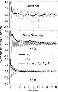
Figure 1: Autocorrelation functions of the sequences under study arbitrary assuming the sampling step $\Delta t$ as being expressed in seconds. The upper part exhibits the autocorrelation in the three solutions of the Lorenz map, while the lower part shows the autocorrelation in each of the seven sequences yielded from the Chang-Shirer map in both $r=28$ and $r=56$ cases.

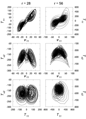
Figure 2: Some projections of the Chang-Shirer attractors corresponding to $r=28$ on the left and $r=56$, on the right in case of $\Delta t=0.01$.

3 Sequences used in the present analysis

The methods, shortly described in the previous section are commonly used to judge whether a time series represents one-dimensional projection of a chaotic system or not. To test their sensitivity to detect chaos in a complex system, they were applied to each of the sequences obtained as solutions of a 7D map taken to mimic a system characterised by a higher extent of complexity. Simultaneously, a 3D map considered an example of a less complex system was a subject of the same studies for comparison. The well known Lorenz map (Lorenz, 1963) defined as:

$$\dot{X} = \sigma(Y-X)$$

$$\dot{Y} = X(\rho-Z)-Y$$ (11)

$$\dot{Z} = XY-\beta Z$$

where $\sigma=10,\,\rho=28$ and $\beta=8/3$, has been chosen to represent this case. The former system was presented by a map defined by Chang and Shirer (1984) as (hereinafter referred to as the Chang-Shirer map or system):

$$\dot{\psi}_{m1}=aC_{5}C_{7}\psi_{n1}\psi_{(m-n)2}/4C_{1}$$

$$+PmaT_{m1}/C1-PC_{1}\psi_{m1}$$

$$\dot{\psi}_{n1}=-aC_{5}C_{6}\psi_{m1}\psi_{(m-n)2}/4C_{2}$$

$$+PnaT_{n1}/C_{2}-PC_{2}\psi_{n1}$$

$$\dot{\psi}_{(m-n)2}=-a^{3}C_{4}C_{5}^{2}\psi_{m1}\psi_{n1}/4C_{3}$$

$$+PaC_{4}T_{(m-n)2}/C_{3}-PC_{3}\psi_{(m-n)2}$$

$$\dot{T}_{m1}=aC_{5}[\psi_{n1}T_{(m-n)2}-\psi_{(m-n)2}T_{n1}]/4$$ (12)

$$+ma\psi_{m1}T_{o2}+maR\psi_{m1}-C_{1}T_{m1}$$

$$\dot{T}_{n1}=aC_{5}[\psi_{m1}T_{(m-n)2}+\psi_{(m-n)2}T_{m1}]/4$$

$$+na\psi_{n1}T_{o2}+naR\psi_{n1}-C_{2}T_{n1}$$

$$\dot{T}_{(m-n)2}=-aC_{5}[\psi_{m1}T_{n1}+\psi_{n1}T_{m1}]/4$$

$$+aC_{4}R\psi_{(m-n)2}-C_{3}T_{(m-n)2}$$

$$\dot{T}_{o2}=-a[m\psi_{m1}T_{m1}+n\psi_{n1}T_{n1}]/2-4T_{o2}\,,$$

where $C_{1}=1+m^{2}a^{2},\,C_{2}=1+n^{2}a^{2},\,C_{3}=4+(m-n)^{2}a^{2},\,C_{4}=m-n,\,C_{5}=m+n,\,C_{6}=3+C_{4}^{2}a^{2}-m^{2}a^{2}$ and $C_{7}=3+C_{4}^{2}a^{2}-n^{2}a^{2}$. Analysing this system, Nese et al. (1984) found that for $m=2,\,n=1,\,a=\sqrt{2}/2,\,P=10$ and $R=6.75\,r$ it provides chaotic solutions.

The three sequences given by the Lorenz map and two groups of sequences obtained from the Chang-Shirer map (Nese et al., 1984) for (i) $r=28$ and initial conditions (100, -150, -100, -1200, -2000, -5000, -2500), and (ii) $r=56$ with initial vector (-6, 20, -15, 10, 5, 15, 16) were obtained with sampling steps $\Delta t=0.01,\,0.05,\,0.1\,\,\text{and}\,\,0.5$, respectively. All these solutions have been found by using the “ode45” MATLAB procedure for 20000 sampling steps, omitting the first 10000 to avoid transitions. The sampling size of $N=10000$ was taken to satisfy inequality (10) (see also Table 1) despite some objections to the claim about the minimal sampling size (Grassberger et al., 1991).

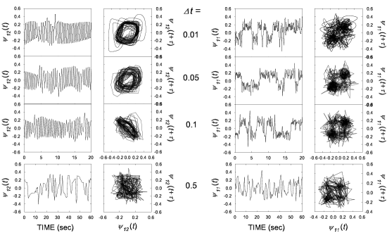
Figure 3: The two columns on the left present the time series and 2D projections of the corresponding attractors reconstructed from $\psi_{12}(r=28)$ for different steps $\Delta t$ indicated in the central part of the figure. The right two columns exhibit the same for $\psi_{11}(r=56)$.

Table 1: The three Lyapunov exponents of the Lorenz map and the largest five ones computed for the Chang-Shirer system for $r=28$ and $r=56$, respectively together with the Kaplan-Yorke ($D_{KY}$) and correlation ($D_{2}$) dimensions of the attractors, all evaluated by Nese et al. (1984) and considered reference values in the present analysis. The Lyapunov exponents are given in $\bigl{(}$(bits/sec)$\cdot$ln2$\bigr{)}$.

$\lambda_{1}$	$\lambda_{2}$	$\lambda_{3}$	$\lambda_{4}$	$\lambda_{5}$	$D_{KY}$	$D_{2}$
Lorenz map
$0.93$	$0.0$	$-14.60$	—	—	$2.063$	$2.05\pm 0.01$
Chang-Shirer map, $r=28$
$0.84$	$0.07$	$0.00$	$-0.43$	$-18.60$	$4.03$	$2.9\pm 0.1$
Chang-Shirer map, $r=56$
$2.51$	$1.12$	$0.00$	$-1.80$	$-16.30$	$4.11$	$3.8\pm 0.1$

Figure 1 presents the autocorrelation functions for these three groups of sequences adopted for the present analysis. It is seen that the time series presented by $\psi_{11}$ in both $r=28$ and $r=56$ cases and, $T_{11}$ for $r=28$ are characterised by comparatively high autocorrelation.

Some 2D projections of the Chang-Shirer attractors constructed for $r=28$ and $r=56$ respectively, are shown in Fig. 2, while Fig. 3 exhibits the reconstructed attractors from $\psi_{12}(r=28)$ and $\psi_{11}(r=56)$ corresponding to different sampling steps $\Delta t$. Each of the sequences under study has been normalized by $\bigl{(}\max(x_{i})-\min(x_{i})\bigr{)}_{1\leq i\leq N}$ that limits the differences $|x_{i}-x_{j}|_{1\leq i,j\leq N}$ between 0 and 1, and facilitate the calculation of the parameters used in the analysis. Figure 3 shows that the time series patterns found for $\Delta t=0.05$ and 0.1 do not differ significantly from those at $\Delta t=0.01$ in both cases shown on the left and right, while for $\Delta t=0.5$ the corresponding sequences look completely different. However, the corresponding 2D phase portraits indicate that the reconstructed attractors are more sensitive to the variations in the sampling time $\Delta t$. It is clearly seen that only for $\Delta t=0.01$ the projections of the reconstructed attractors are depicted by smooth curves like those presented in Fig. 2. For lower resolution (higher $\Delta t$) the attractors turn out to be represented by broken-line orbits and for $\Delta t=0.5$ the fiducial trajectory is composed in practice by long segments. A similar loss of the typical features of the attractor, resulted from enlarging of the sampling time, was reported by Kim and Yoon (2001) who analysed the Lorenz map. Thus, it can be concluded that an attractor projection depicted by broken-line orbits acts as an indicator for large sampling step in the sequence under study. However, it should be pointed out that the noise is able to produce a similar effect (Kawata et al., 1997).

Table 2: Minimum embedding dimension $m_{K}$ found for each of the attractors reconstructed using the sequences under study, determined as $m_{K}=\min\,(m:\text{FNNP}<1\%)$. The values found in case when FNNP follows the noise contaminated pattern (see Fig. 4 and the text), determined as $m_{K}=\min\,(m:\text{FNNP}<n\%)$ are signed by an asterisk together with the lowest value $n\%$ of FNNP, if it exceeds 1%, given in parenthesis. The cases for which FNNP behaves similarly to a stochastic sequence shown in Fig. 4 are signed by “–”. The values of $m_{GP}$ are also given, separated from $m_{K}$ by semicolons; “$\infty$” indicates that the corresponding value can not be determined varying $m$ from 1 to 20.

$\Delta t=$	0.01	0.05	0.1	0.5
Lorenz map
$X$	3; 3	3; 3	3; 3	3; 3
$Y$	3; 3	3; 3	3; 3	3; 3
$Z$	3; 3	3; 3	3; 3	4; 3
Chang–Shirer map, r=28
$\psi_{21}$	4; 7	5; 7	$4^{\ast}$(2%); 7	–;$\infty$
$\psi_{11}$	4; $\infty$	5; 7	5; 4	–;$\infty$
$\psi_{12}$	4; 4	4; 5	4; 5	4; 7
$T_{21}$	4; 7	4; 7	4; 7	4;$\infty$
$T_{11}$	6,$\infty$	$11^{\ast}$(2%); $\infty$	4; 6	4; 6
$T_{12}$	4; 4	$4^{\ast}$; 4	$4^{\ast}$; 5	–; 6
$T_{o2}$	4; 4	4; 5	4; 5	4;$\infty$
Chang–Shirer map, r=56
$\psi_{21}$	5; 7	$5^{\ast}$(3%); 7	$5^{\ast}$(3%); 7	–;$\infty$
$\psi_{11}$	6; $\infty$	4;$\infty$	–;$\infty$	–;$\infty$
$\psi_{12}$	7; 5	4; 7	4; 6	4;$\infty$
$T_{21}$	4; 6	4; 6	4; 6	4;$\infty$
$T_{11}$	5; 7	4; 7	4; 7	4;$\infty$
$T_{12}$	4; 6	4; 7	4; 7	4;$\infty$
$T_{o2}$	10; 7	$4^{\ast}$(5%); 6	$4^{\ast}$(5%); 6	4;$\infty$

Table 1 gives the Lyapunov spectra, Kaplan-Yorke ($D_{KY}$) and correlation ($D_{2}$) dimensions estimated by Nese et al. (1984) for the attractors corresponding to Lorenz and two cases of the Chang-Shirer systems, which values have been used here as reference ones.

4 Results and discussion

Table 2 exhibits the minimum embedding dimensions $m_{K}$ and $m_{GP}$ of the attractors, reconstructed from the sequences under study. As can be seen, for the Lorenz attractor the FNNP approach gave an estimation of $m_{K}$ equal to the real embedding dimension $m_{L}=3$, with one exception slightly exceeding this value. Conversely, the estimates found for the two groups of the time series obtained from Chang-Shirer system in case of $r=28$ and $r=56$ respectively, showed values varying between 4 and 11. Figure 4 represents the behaviour of FNNP as a function of the embedding dimension for $\psi_{21}(r=56)$ obtained for different time resolutions. The curve corresponding to the sequence with sampling time of 0.01 drops to 0.73% at $m=5$ and remains below this value until embedding dimension increases up to 20. A similar behaviour showed FNNP in all cases of the time series $X$, $Y$ and $Z$ obtained from the Lorenz system. The FNNP curve found for $\psi_{21}(r=56,\Delta t=0.05)$ follows a comportment similar to that presented by noise contaminated time series, while the curve characterising $\psi_{21}(r=56,\Delta t=0.5)$ shows a behaviour typical for the attractor reconstructed from a stochastic time series. Table 2 shows that both $m_{K}$ and $m_{GP}$ estimators give in practice equal values for the attractors of the Lorenz system, except for $Z(\Delta t=0.5)$ where a slight difference between them is seen. However, the application of the same approaches to the sequences yielded from the Chang-Shirer system do not give such an accordance between $m_{K}$ and $m_{GP}$ estimates. It is seen that $m_{K}$ tends to be underestimated and only in case of $\psi_{12}(r=56,\Delta t=0.01)$, $m_{K}$ represents the actual embedding dimension $m_{CS}=7$. In contrast, $m_{GP}=m_{CS}$ for 32% of all the sequences obtained from the Chang-Shirer map for the adopted values of $\Delta t$ but for 30% of them the corresponding approach does not give an estimate, while such a percentage is 11 % for the FNNP method.

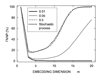
Figure 4: The false nearest neighbors percentage (FNNP) found as a function of embedding dimension for $\psi_{21}(r=56)$ in case of three different sampling times $\Delta t$ equal to 0.01, 0.05 and 0.5, respectively. The FNNP determined for a sequens of random values with Gaussian distribution, considered to represent a stochastic process is also given for comparison. In all cases the parameter $R_{tol}$ was assumed to be equal to 30.

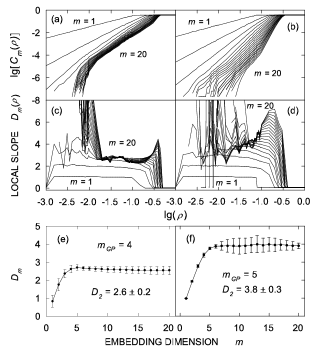
Figure 5: Behaviour of the correlation integral $C_{m}(\rho)$ as a function of $\rho$ presented in decimal logarithm scale (a, b) and the corresponding local slope $D_{m}(\rho)$ (c, d) evaluated for the sequence $\psi_{12}(r=28,\,\Delta t=0.01)$ (left) and $\psi_{12}(r=56,\,\Delta t=0.01)$ (right). In both cases the embedding dimension $m$ gradually increased from 1 to 20. Panels (e, f) present the behaviour of the parameter $D_{m}$ as a function of $m$ and the corresponding values of $m_{GP}$ and $D_{2}$ are also indicated.

Figure 5 shows as an example the scaling behaviour of the correlation integral $C(\rho)$ as a function of $\rho$ in decimal logarithm scale and the corresponding variations in the local slop $D_{m}(\rho)$ for $\psi_{12}(\Delta t=0.01)$ obtained assuming $r=28$ and $r=56$, respectively. The lower part of Fig. 5 illustrates the behaviour of parameter $D_{m}$ defined from the curves $D_{m}(\rho)$ $\bigl{(}$see Eq. (6)$\bigl{)}$. It can be seen that both cases presented in Fig. 5 exhibit different scaling patterns of the correlation integral. Panels (c) and (d) indicate that the linear part is easy recognizable for $r=28$, while for $r=56$ it becomes shorter and less marked. Figure 6 illustrates the comportment of the correlation integral evaluated for $\psi_{11}(r=28,\,\Delta t=0.05)$, one of the sequences characterised by high autocorrelation (see Fig. 1). Assuming $W=1$, Eqs. (2.3) and (6) give the curves shown on the left-hand side of Fig. 6, while the curves corresponding to $W=\tau=32$ can be seen on the right. The figure indicates that a linear segment of $\lg\bigl{(}C(\rho)\bigr{)}$ can not be identified for $W=1$, while taking $W=32$ a very short plateau in the local slope could be recognized for $-1.3<\lg(\rho)<-0.8$. However, despite the use of the cutoff parameter $W$ the behaviour of the correlation integral slightly changes that makes the estimation of the correlation dimension to be on the edge of the reliability. In contrast, the three series yielded by the Lorenz system for the adopted values of $\Delta t$ show a comparatively long linear segment in the corresponding curves similarly to the case given in Figs. 5 (a) and (c).

Table 3: Estimators of the Hausdorff dimension $D_{0}$ of the attractors under study presented by the corresponding correlation dimension $D_{2}$ with its standard deviation $\Delta D_{2}$ and the Kaplan-Yorke dimension $D_{KY}$ both shown as “$D_{2}\pm\Delta D_{2};\,D_{KY}$”. The symbol “$\infty$” indicates that a finite value of $D_{2}$ has not been found for embedding dimension increasing up to 20.

$\Delta t=$	0.01	0.05	0.1	0.5
Lorenz map
$X$	2.07$\pm$0.09; 2.3	2.06$\pm$0.04; 2.4	2.05$\pm$0.08; 2.5	2.05$\pm$0.08; 2.9
$Y$	2.08$\pm$0.09; 2.3	2.04$\pm$0.09; 2.3	2.05$\pm$0.05; 2.2	2.05$\pm$0.08; 2.9
$Z$	2.10$\pm$0.08; 2.1	2.08$\pm$0.06; 2.2	2.17$\pm$0.07; 2.4	2.10$\pm$0.08; 2.6
Chang–Shirer map, r=28
$\psi_{21}$	2.7$\pm$0.2; 4.8	3.1$\pm$0.2; 4.6	3.2$\pm$0.1; 4.6	$\infty$; 5.1
$\psi_{11}$	$\infty$; 4.8	3.3$\pm$0.6; 4.3	2.3$\pm$0.4; 5.3	$\infty$; 4.6
$\psi_{12}$	2.6$\pm$0.2; 4.6	3.2$\pm$0.2; 4.3	3.3$\pm$0.2; 4.6	3.7$\pm$0.2; 4.6
$T_{21}$	2.6$\pm$0.1; 4.6	3.2$\pm$0.2; 4.6	3.2$\pm$0.2; 4.9	$\infty$; 4.6
$T_{11}$	$\infty$; 4.4	$\infty$; 4.3	3.5$\pm$0.5; 4.4	3.7$\pm$0.6; 4.6
$T_{12}$	2.6$\pm$0.1; 4.6	3.0$\pm$0.3; 4.5	3.3$\pm$0.2; 4.5	3.7$\pm$0.2; 4.7
$T_{o2}$	2.8$\pm$0.1; 4.4	3.3$\pm$0.1; 4.8	3.3$\pm$0.1; 4.4	$\infty$; 4.4
Chang–Shirer map, r=56
$\psi_{21}$	3.9$\pm$0.2; 4.4	3.7$\pm$0.2; 4.7	3.9$\pm$0.1;1,4.8	$\infty$; 4.1
$\psi_{11}$	$\infty$; 5.1	$\infty$; 4.5	$\infty$; 3.0	$\infty$; 3.6
$\psi_{12}$	3.8$\pm$0.3; 4.5	3.9$\pm$0.2; 4.5	3.9$\pm$0.1; 4.4	$\infty$; 3.4
$T_{21}$	3.9$\pm$0.1; 4.6	3.8$\pm$0.3; 4.6	3.9$\pm$0.1; 4.6	$\infty$; 3.5
$T_{11}$	3.7$\pm$0.1; 4.5	3.8$\pm$0.1; 4.6	4.0$\pm$0.1; 4.6	$\infty$; 3.7
$T_{12}$	3.8$\pm$0.4; 4.7	3.8$\pm$0.1; 4.3	3.9$\pm$0.1; 4.3	$\infty$; 3.6
$T_{o2}$	3.9$\pm$0.2; 4.5	4.1$\pm$0.2; 4.5	4.0$\pm$0.1; 4.6	$\infty$; 3.5

The behaviour of the correlation integral presented in the upper part of Fig. 5 reveals an interesting feature. The increasing slope at low $\rho$ significantly more pronounced for $r=28$ lead to assume the presence of noise in the corresponding attractors (Theiler, 1990; Eckmann and Ruelle, 1985) even though such a component was not added solving Eqs. (3). A similar conclusion can be made analysing the behaviour of FNNP as a function of the embedding dimension $m$ for some of the sequences yielded from the Chang-Shirer map as Fig. 4 and Table 2 show. It should be pointed out that an analogous occurrence was not observed studding the 3D Lorenz system.

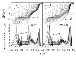
Figure 6: Scaling behaviour of the correlation integral $C_{m}(\rho)$ as a function of $\rho$ in decimal logarithm scale (upper panels) and the corresponding local slope $D_{m}(\rho)$ (lower panels) assessed for the time-series $\psi_{11}(r=28,\,\Delta t=0.05)$ for two different values of parameter $W$ (see Eq. 2.3).

Table 3 exhibits the correlation dimension $D_{2}$ of the attractors reconstructed from the time series under study. It can be seen that the values of $D_{2}$ found for the sequences of the Lorenz system for all adopted sampling steps are very close to the reference ones given in Table 1 . A similar behaviour shows the correlation dimensions $D_{2}$ of the Chang-Shirer attractors reconstructed for $r=56$ and $\Delta t=0.01,\,0.05$ and 0.1. For $r=28$ Table 3 exhibits a slight increase of $D_{2}$ when $\Delta t$ increases. Surprisingly, Table 3 indicates also that some of the series provided by the Chang-Shirer system determine an attractor for which a finite correlation dimension cannot be found. In case of $r=56$ the parameter $D_{2}$ is infinite for $\psi_{11}$ found at all adopted $\Delta t$, while for $\Delta t=0.5$ such an occurrence characterises all the sequences. In case of $r=28$ the attractors with undefined correlation dimension are those constructed from $\psi_{11}$ for $\Delta t=0.01$ and 0.5, and $T_{11}$ for $\Delta t=0.01$ and 0.05. For $\Delta t=0.5$ such features show also $\psi_{21}$, $T_{21}$ and $T_{02}$. It should be pointed out that the assessment of the correlation dimension $D_{2}$ for $\psi_{11}(r=28,\,\Delta t=0.1)$ and $T_{11}(r=28,\,\Delta t=0.1,\,\,\text{and}\,\,0.5)$ was very difficult to make, like in the case of $\psi_{11}(r=28,\,\Delta t=0.05)$ shown in Fig. 6.

Table 4: Lyapunov exponents of the Lorenz system obtained from the analysis of the corresponding sequences, arbitrary assuming $\Delta t$ in seconds.

	$\lambda_{1}$	$\lambda_{2}$	$\lambda_{3}$
$\Delta t=0.01$ s
X	0.98$\pm$0.07	0.0	-3.30$\pm$0.60
Y	1.09$\pm$0.04	0.0	-3.20$\pm$0.10
Z	0.94$\pm$0.09	0.0	-6.10$\pm$0.20
$\Delta t=0.5$ s
X	1.00$\pm$0.10	0.0	-1.10$\pm$0.70
Y	1.12$\pm$0.02	0.0	-1.26$\pm$0.09
Z	0.89$\pm$0.09	0.0	-1.50$\pm$0.60

Tables 4 and 5 represent the Lyapunov spectra of the sequences obtained from the Lorenz and Chang-Shirer sistems, respectively. As can be seen the positive Lyapunov exponents evaluated for the attractors of the Lorenz system in case of $\Delta t=0.01$ and 0.5 are in good agreement with the reference values given in Table 1. Similar results, not shown in Table 4, were found for 0.05 and 0.1 sampling steps, as well. Table 5 exhibits the five largest Lyapunov exponents found for all the seven sequences yielded from the Chang-Shirer system at $\Delta t=0.01$ and 0.5 for both $r=28$ and $r=56$ values. In case of $r=28$ and $\Delta t=0.01$ the positive exponents turn out to be overestimated except for the sequences $\psi_{11}$ and $T_{11}$. The same features present the time series found for 0.05 and 0.1 sampling times (not shown in Table 5). In contrary, for $\Delta t=0.5$ the exponent $\lambda_{1}$ turned out to be underestimated. Except for $\psi_{11}$, the positive values of $\lambda_{l}$ have been correctly estimated for all the sequences obtained for $r=56$ at sampling times $\Delta t=0.01,\,0.05$ and 0.1 (the last two cases are not shown in Table 5), while for $\Delta t=0.5$ the assessments of the Lyapunov exponents give completely different results characterised by one, appreciably underestimated positive exponent.

Table 5: The first five Lyapunov exponents evaluated from the Chang-Shirer sequences for both adopted values of parameter $r$ and sampling steps of 0.01 and 0.5, arbitrary assuming $\Delta t$ in seconds.

	$\lambda_{1}$	$\lambda_{2}$	$\lambda_{3}$	$\lambda_{4}$	$\lambda_{5}$
r=28
$\Delta t=0.01$ s
$\psi_{21}$	1.27$\pm$0.06	0.43$\pm$0.06	0.0	-0.60$\pm$0.20	-1.40$\pm$0.40
$\psi_{11}$	0.51$\pm$0.03	0.15$\pm$0.02	0.0	-0.15$\pm$0.01	-0.62$\pm$0.05
$\psi_{12}$	1.40$\pm$0.10	0.60$\pm$0.10	0.0	-0.65$\pm$0.02	-2.40$\pm$0.10
$T_{21}$	1.30$\pm$0.09	0.55$\pm$0.03	0.0	-0.70$\pm$0.10	-2.00$\pm$0.20
$T_{11}$	0.36$\pm$0.07	0.22$\pm$0.06	0.0	-0.31$\pm$0.02	-0.71$\pm$0.03
$T_{12}$	1.40$\pm$0.10	0.70$\pm$0.10	0.0	-0.75$\pm$0.09	-2.10$\pm$0.10
$T_{o2}$	1.22$\pm$0.06	0.60$\pm$0.10	0.0	-0.80$\pm$0.10	-2.81$\pm$0.03
$\Delta t=0.5$ s
$\psi_{21}$	0.19$\pm$0.06	0.06$\pm$0.02	0.0	-0.07$\pm$0.01	-0.14$\pm$0.02
$\psi_{11}$	0.18$\pm$0.03	0.07$\pm$0.02	0.0	-0.12$\pm$0.02	-0.23$\pm$0.01
$\psi_{12}$	0.26$\pm$0.05	0.11$\pm$0.02	0.0	-0.16$\pm$0.02	-0.35$\pm$0.01
$T_{21}$	0.13$\pm$0.03	0.03$\pm$0.01	0.0	-0.07$\pm$0.01	-0.15$\pm$0.01
$T_{11}$	0.18$\pm$0.03	0.07$\pm$0.01	0.0	-0.11$\pm$0.02	-0.21$\pm$0.02
$T_{12}$	0.26$\pm$0.09	0.12$\pm$0.06	0.0	-0.13$\pm$0.02	-0.33$\pm$0.03
$T_{o2}$	0.16$\pm$0.04	0.05$\pm$0.02	0.0	-0.13$\pm$0.02	-0.22$\pm$0.01
r=56
$\Delta t=0.01$ s
$\psi_{21}$	2.60$\pm$0.20	1.70$\pm$0.10	0.0	-2.30$\pm$0.50	-4.50$\pm$0.30
$\psi_{11}$	0.59$\pm$0.07	0.33$\pm$0.04	0.0	-0.24$\pm$0.04	-0.55$\pm$0.08
$\psi_{12}$	2.60$\pm$0.20	1.51$\pm$0.04	0.0	-2.10$\pm$0.10	-4.30$\pm$0.10
$T_{21}$	2.70$\pm$0.30	1.40$\pm$0.30	0.0	-1.26$\pm$0.09	-4.50$\pm$0.50
$T_{11}$	2.60$\pm$0.20	1.50$\pm$0.10	0.0	-2.00$\pm$0.50	-4.00$\pm$0.30
$T_{12}$	2.20$\pm$0.40	1.10$\pm$0.30	0.0	-1.20$\pm$0.20	-2.90$\pm$0.20
$T_{o2}$	2.70$\pm$0.30	1.20$\pm$0.10	0.0	-1.60$\pm$0.10	-4.50$\pm$0.30
$\Delta t=0.5$ s
$\psi_{21}$	0.60$\pm$0.20	0.0	-0.17$\pm$0.01	-0.38$\pm$0.05	-1.00$\pm$0.40
$\psi_{11}$	0.58$\pm$0.09	0.0	-0.21$\pm$0.04	-0.60$\pm$0.04	-1.43$\pm$0.01
$\psi_{12}$	0.50$\pm$0.10	0.0	-0.24$\pm$0.01	-0.64$\pm$0.03	-1.39$\pm$0.07
$T_{21}$	0.54$\pm$0.07	0.0	-0.24$\pm$0.02	-0.55$\pm$0.09	-1.42$\pm$0.03
$T_{11}$	0.50$\pm$0.10	0.0	-0.15$\pm$0.02	-0.48$\pm$0.03	-1.38$\pm$0.06
$T_{12}$	0.24$\pm$0.01	0.0	-0.09$\pm$0.01	-0.26$\pm$0.02	-0.67$\pm$0.05
$T_{o2}$	0.49$\pm$0.08	0.0	-0.22$\pm$0.03	-0.59$\pm$0.04	-1.37$\pm$0.03

In all cases the last component of the Lyapunov spectra turned out to be significantly overestimated due to the limited ability of the method to estimate correctly the negative exponents (Zeng et al., 1992b). Such an overestimation caused a corresponding overestimation of the Kaplan-Yorke dimension $D_{KY}$ (see Table 1 and Table 3). For the Lorenz system, the parameter $D_{KY}$ was found to be higher by 2%–40% with respect to the reference values given in Table 1, while such an amount for the Chang-Shirer system varied from 9% to 20% for $r=28$ and from 5% to 14% for $r=56$, respectively. On the other hand, the dimension $D_{KY}$ has been determined in practice for each of the attractors and, when the correlation dimension $D_{2}$ exists, the relationship between them, expressed by inequalities (9) is always held. In case of the Chang-Shirer system, except for the sequences at $r=56$ and $\Delta t=0.5$, and for $\psi_{11}(r=56,\,\Delta t=0.1)$, all the estimates of $D_{KY}$ are very similar to each other even in the cases when the Lyapunov exponents were not correctly evaluated. Thus, it can be concluded that $D_{KY}$ is slightly sensitive to the internal features of the system that could impact the other estimators analysed here, on the one hand, and to the variations in the sampling step, on the other.

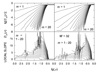
Figure 7: As in Fig. 6 but for surrogates of $\psi_{12}(r=56,\,\Delta t=0.01)$ (left) and $\psi_{11}(r=28,\,\Delta t=0.05)$ (right).

To have more clear idea about the characteristics of the attractors reconstructed from the time series under study, the corresponding surrogate sequences were created as was described in Section 2.5. Figure 7 illustrates the behaviour of the correlation integral calculated for surrogates corresponding to $\psi_{12}(r=56,\,\Delta t=0.01)$ and $\psi_{11}(r=28,\,\Delta t=0.05)$. Comparing the curves of Fig. 7 with those presented in Fig. 5 (upper right part) and Fig. 6 (right) respectively, that concern the original sequences, it can be seen that the surrogates exhibit quite different patterns. Hence, despite of the hardly recognizable linear segment in the curves $C_{m}(\rho)$ corresponding to the original sequences $\psi_{12}(r=56,\,\Delta t=0.01)$ and $\psi_{11}(r=28,\,\Delta t=0.05)$ it can be conclude that we deal with time series provided by a chaotic system.

The results presented in Tables 2, 3 and 5 identify some of the sequences under study as particular cases. To understand better the behaviour of these sequences, except for the correlation dimension $D_{2}$, the Lyapunov spectrum $\lambda_{l}$ and minimum embedding dimension $m_{K}$ of the corresponding surrogate attractors have been also evaluated. While the parameter $D_{2}$ showed features similar to those given in Fig. 7 (not shown here), the results for $\lambda_{l}$ and $m_{K}$ presented some particularities. Figures 8 and 9 demonstrate the estimates of these parameters for some cases of $\psi_{11}$ and $\psi_{21}$ together with the $Y$ component of the Lorenz system. For the latter, it is seen that the surrogate data present different patterns of $\lambda_{l}$ and $m_{K}$ respectively, for both $\Delta t=0.01$ and $\Delta t=0.1$ (see Figs. 8 and 9). Similarly, the Lyapunov spectra for $\psi_{21}$ sequences and the corresponding surrogates are different. Despite of the same embedding dimension, identified as 5 for both original and surrogate sequences $\psi_{21}(\Delta t=0.05\,\,\text{and}\,\,0.1)$ as Fig. 9 shows, the surrogate FNNP behaves similarly to a noise-free time series, while it follows the noise-contaminated comportment for the original sequences (see Fig. 4). Only the first positive component of the Lyapunov spectra for $\psi_{11}(r=28)$ and the corresponding surrogates in both $\Delta t=0.01$ and $\Delta t=0.05$ cases are different (Fig. 8), while the FNNP approach shows no differences between $\psi_{11}(r=28)$ sequences and their surrogates (Fig. 9). The Lyapunov spectra of $\psi_{11}(r=56,\,\Delta t=0.05\,\,\text{and}\,\,0.1)$ for both original and surrogate sequences are almost equal to each other (Fig. 8). For surrogate of $\psi_{11}(r=56,\,\Delta t=0.05)$, FNNP behaves similarly to the original sequence as Fig. 9 indicates, while the surrogate of $\psi_{11}(r=56,\,\Delta t=0.1)$ exhibits a behaviour quite different from the corresponding original sequence. In fact, while for the original data FNNP shows a typical for stochastic time series comportment, the corresponding surrogate data present a FNNP behaviour characterising a noise-free chaotic time series.

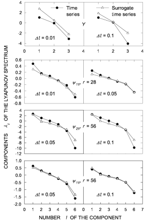
Figure 8: Lyapunov exponents for some of the time series determined by the Lorenz and Chang-Shirer systems together with the values found for the corresponding surrogate data.

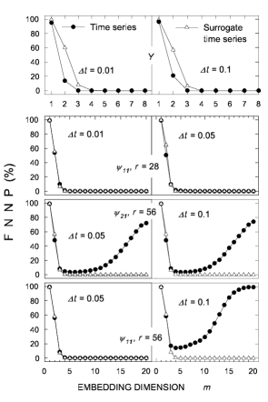
Figure 9: Variations in the false nearest neighbors percentage (FNNP) for the same as in Fig. (8) sequences.

Thus, while for the 3D Lorenz map the conclusion about chaotic character of the system was quite straightforward, for the Chang-Shirer map some of the sequences ran into difficulties. In fact, let we assume that a blind test using the sequences yielded from the second map should be performed. If we make a conclusion about chaotic origin just on the basis of the estimated correlation dimension $D_{2}$ we will take the wrong decision attributing stochastic features to considerable number of the sequences. In addition for instance, if $\psi_{11}(r=28,\,\Delta t=0.01)$ is the subject of the analysis, the adopted methods give $m_{K}=4$, undefined $m_{GP}$, $D_{2}=\infty$, $D_{KY}=4.8$, and two positive Lyapunov exponents $\lambda_{1}=0.51\pm 0.03$ and $\lambda_{2}=0.15\pm 0.02$. The surrogate test shows differences just in the first Lyapunov exponent and, as a result in $D_{KY}$, which are $0.29\pm 0.03$ and 5.1, respectively. Thus, if a researcher had at his/her disposal these estimates, he/she would likely conclude that the system, which generated this series is stochastic. In case of $\psi_{11}(r=56,\,\Delta t=0.05)$ such a decision would seem more grounded. Since a noise component was not added solving the analysed maps and the sampling size of the sequences was chosen to satisfy the conditions assumed to assure a correct estimation of the invariants, it could be concluded that the difficulties in detecting chaos have arisen likely due to specific internal features of the 7D system. It should be pointed out that the last two examples showing that the chaotic origin of the corresponding sequences is hardly recognizable concerned the system components, characterised by high autocorrelation as Fig. 1 shows.

The results reported by Zeng et al. (1992a) illustrate behaviour similar to that described in this section. The authors examined the sequences yielded from surface temperature and pressure measurements. The analysis showed infinite or unreliably high correlation dimension of the reconstructed attractors. On the other hand, it was found that these attractors were characterised by two positive Lyapunov exponenets and despite that the Kaplan-Yorke dimension was not evaluated, it is easy to conclude that $D_{KY}$ varies between 4 and 5. Although the question about chaotic origin of the sequences was not raised by Zeng et al. (1992a), the results of the present study allow the conclusion that the time series analysed by them had been likely generated by chaotic processes.

5 Conclusions

The parameters, most commonly used to judge whether a time series represents one-dimensional projection of a chaotic system have been estimated for each of the sequences generated by both 3D Lorenz and 7D Chang-Shirer maps considering the second as a more complex system. The sequences were not contaminated by additional noise and their sampling sizes were assumed to assure a correct estimation of the correlation dimension and Lyapunov exponents. In addition, the impact of the sampling step on the assessed parameters was investigated.

Performed analysis highlighted some important features of the reconstructed attractors. First of all, the adopted methods gave an unambiguous answer to the question if each of the sequences provided by the 3D Lorenz map has a chaotic origin. Moreover, the estimated parameters showed very similar values for all sampling times, assumed here. In contrary, not each of the sequences yielded from the 7D map represented correctly the attractor properties as in the case of the 3D system. For some of the sequences of the 7D map the false nearest neighbors approach together with the correlation integral behaviour characterised the system as stochastic especially in the case of larger sampling steps. When these approaches gave an assessment, the minimum embedding dimension turned out to be generally underestimated, while the correlation dimension $D_{2}$ was predominantly correctly evaluated. For the 7D sequences characterised by high autocorrelation, a finite value of $D_{2}$ was impossible to find in the most of the cases and the corresponding positive Lyapunov exponents $\lambda_{l}^{+}$ turned out to be underestimated. A similar estimates of $D_{2}$ and $\lambda_{l}^{+}$ were obtained for the time series with large sampling step. Among all the evaluated parameters just the Kaplan-Yorke estimator $D_{KY}$ of the Housdorff dimension of the attractor gave reliable values for the major part of the sequences yielded from the 7D map. The surrogate data test applied to some time series did not show differences between certain parameters evaluated for the original and the corresponding surrogate sequences, that usually characterises a stochastic system.

The present study shows that the widely used methods for detecting chaos in systems of the real world could run into difficulties with a sequence generated by a high-dimensional process even in case when it is yielded from a theoretical map without noise contamination and presenting a sufficient sampling size. Thus, it can be concluded that the decision about chaotic origin of a time series provided by an experiment or field observations should be taken with a special caution, taking into account the estimations of several parameters that characterise the corresponding attractor. Even if only one or two of these parameters give a positive answer, the hypothesis about chaotic origin of the time series should not be excluded.

References

- Cao (1997) Cao, L., 1997. Practical method for determining the minimum embedding dimension of a scalar time series. Physica D 110, 43–50 (see Introductin).
- Chang and Shirer (1984) Chang, H.R., Shirer, H.N., 1984. Transitions in shallow convection: an explanation for lateral cell expansion. J Atmos. Sci. 41, 2334–2346.
- Eckmann et al. (1986) Eckmann, J.P., Kamphorst, S.O., Ruelle, D., Ciliberto, S., 1986. Liapunov exponents from time series. Phys Rev A 34, 4971–4979.
- Eckmann and Ruelle (1985) Eckmann, J.P., Ruelle, D., 1985. Ergodic theory of chaos and strange attractors. Rev. Mod. Phys. 57, 617–656.