Extreme variability in convergence to structural balance in frustrated dynamical systems

Abstract

In many complex systems, the dynamical evolution of the different components can result in adaptation of the connections between them. We consider the problem of how a fully connected network of discrete-state dynamical elements which can interact via positive or negative links, approaches structural balance by evolving its links to be consistent with the states of its components. The adaptation process, inspired by Hebb’s principle, involves the interaction strengths evolving in accordance with the dynamical states of the elements. We observe that in the presence of stochastic fluctuations in the dynamics of the components, the system can exhibit large dispersion in the time required for converging to the balanced state. This variability is characterized by a bimodal distribution, which points to an intriguing non-trivial problem in the study of evolving energy landscapes.

Many complex systems that arise in biological, social and technological contexts can be represented as a collection of dynamical elements, interacting via a non-trivial connection topology Newman10 ; Barrat08 . A variety of critical behavior has been observed in such systems, both in the collective dynamics taking place on the network, as well as in the evolution of the network architecture itself Dorogovtsev08 . The interplay between changes to the connection topology (by adding, removing or rewiring links) and nodal dynamics has also been investigated in different contexts Jain01 ; Gross06 ; MacArthur10 ; Durrett12 ; Goudarzi12 ; Liu12 . While the coevolution of network structure and nodal activity has mostly been studied in the simple case where the links are either present or absent, many naturally occurring networks have links with heterogeneously distributed properties. Connections in such systems can differ quantitatively by having a distribution of weights (which may represent the strength of interaction) Barrat04 ; Onnela07 and/or qualitatively through the nature of their interactions, viz., positive (cooperative or activating) and negative (antagonistic or inhibitory) Traag09 . The presence of negative links in signed networks can introduce frustration through the presence of inconsistent relations within cycles in the system Fischer91 . Networks whose positive and negative links are arranged such that frustration is absent are said to be structurally balanced – a concept that was originally introduced in the context of social interactions Heider46 . A classic result in graph theory is that a balanced network can be always represented as comprising two subnetworks, with only positive interactions within each subnetwork, while links between the two are exclusively negative Cartwright56 . Networks of dynamical elements with such structural organization can exhibit non-trivial collective phenomena, e.g., “chimera” order Singh11 .

Recently, the processes through which structural balance can be achieved in networks has received attention from scientists and quantitative models for understanding their underlying mechanisms have been proposed. Evolving networks where the sign of links are flipped to reduce frustration have been shown to reach balance; however, introduction of constraints can sometimes result in jammed states which prevent convergence to the balanced state Antal05 ; Marvel09 . Another approach, using coupled differential equations for describing link adaptation Kulakowski05 , has been analytically demonstrated to result in balance Marvel11 .

While most studies on structural balance have been done in the context of social networks, an important question is whether other kinds of networks, in particular, those that occur in biology, exhibit balance. The recent observation that the resting human brain is organized into two subnetworks that are dynamically anti-correlated (with the activity within each subnetwork being correlated) Fox05 point to the intriguing possibility that the underlying network may in fact be balanced. As connections in the brain evolve according to long-term potentiation which embodies Hebb’s principle Hebb49 , i.e., the link weights change in proportion to the correlation between activity of the connected elements, it suggests a novel process for achieving structural balance. Thus, signed and weighted networks can remove frustration by adjusting the weights associated with the links in accordance with the dynamical states of their nodes. Such a local adaptation process has an intuitive interpretation in social systems, viz., agents that act alike have their ties strengthened, while those behaving differently gradually develop antagonistic relations. In fact, Hebb’s rule may apply more broadly to a large class of systems, for example, in gene regulation networks where it has been suggested that co-expression of genes can lead to co-regulation over evolutionary time-scales Fernando09 .

In this paper, we show that such a link-weight adaptation dynamics can in fact lead to structural balance (shown schematically in Fig. 1), using only local information about the correlation between dynamical states of the nodes. The temporal behavior of the approach to balance shows unexpected features. In particular, we observe that the system exhibits a high degree of variability in the time required to converge to the balanced state when stochastic fluctuations are present in the nodal dynamics. This relaxation time has a bimodal distribution for a range of adaptation rates and noise strengths. Finite-size scaling of the transition from fast to slow relaxation shows that the variation of the scaling exponent is related to the qualitative nature of the way the bimodal distribution emerges. As a larger fraction of positive (negative) interactions reduces (promotes) frustration, we also investigate the role of bias in the sign of interactions on the nature and rate of convergence to the balanced state.

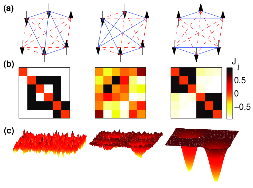
Figure 1: Coevolution of coupling strength with the dynamics on the node starting from a disordered state of spin orientations and interaction strengths randomly selected to be $\pm 1$. (a) The spin configurations in the initial (left), intermediate (center) and final, i.e., after convergence to structural balance (right), states for a system of $N=6$ spins. Solid (broken) lines represent positive (negative) interactions between spins. The corresponding coupling matrices $J$ are shown in (b) while the schematic energy landscapes are represented in (c). The two minima in the balanced state correspond to the pair of degenerate ground states related by reversal of each spin.

We consider a system of $N$ globally coupled Ising spins $\sigma_{i}=\pm 1$ ($i=1,\ldots,N$), the energy for a given configuration of spins being

$$\mathcal{E}=-\sum_{i\neq j}J_{ij}\sigma_{i}\sigma_{j}$$ (1)

where $J_{ij}(=J_{ji})$ is the symmetric bond, representing interaction strength between the spin pair ($i,j$). Structural balance in real social networks have been recently investigated using a similar energy function Facchetti11 . The balanced state corresponds to the situation where the interactions are consistent with the corresponding spin pairs, i.e., $J_{ij}$ and $\sigma_{i}\sigma_{j}$ have the same sign. Starting from a disordered spin configuration and random distribution of interactions, the state of the spins are updated stochastically at discrete time-steps using the Metropolis Monte Carlo (MC) algorithm with temperature $T$. The interaction strengths also evolve after every MC step according to the following deterministic adaptation dynamics:

$$J_{ij}(t+1)=(1-\epsilon)J_{ij}(t)+\epsilon\sigma_{i}(t)\sigma_{j}(t),$$ (2)

where $\epsilon$ governs the rate of change of the interaction relative to the spin dynamics. The $J_{ij}$ dynamics alters the energy landscape on which the state of the spin system evolves. The relaxation time for the system is defined as the characteristic time scale in which the balanced state is reached. Note that the form of Eq. (2) ensures that the relaxation time $\sim 1/\epsilon$ in the absence of any thermal fluctuation (i.e., at $T=0$). Also, it restricts the asymptotic distribution of $J_{ij}$ to the range $[-1,1]$, independent of whether the system converges to a balanced state. In many real systems the signature of the link cannot change, although the magnitude of the link weight can. We have also considered a variant of Eq. (2) for which the dynamics is constrained such that the sign of each $J_{ij}$ cannot change from the initially chosen value. As a result several of the interactions can go to zero when the system relaxes.

In our simulations the initial state of the system for each realization is constructed by choosing the spins $\sigma_{i}$ to be $\pm 1$ with equal probability. For most results shown here, each initial $J_{ij}$ is chosen from a distribution with two equally weighted $\delta$ function peaks at $\pm 1$, i.e., $P(z;\mu)=[(1+\mu)/2]\delta(z-1)+[(1-\mu)/2]\delta(z+1)$ where the mean $\mu=0$. We have verified that the results do not change qualitatively if the initial distribution has a non-zero mean, or has a different functional form (e.g., a uniform distribution in $[-1,1]$), provided that the system is initially far from balance. For each set of parameters ($T,\epsilon$), $10^{4}$ different realizations have been used to statistically quantify the relaxation behavior of the system, which is identified using the energy per bond [Eq.( 1)] normalized by the number of connections, i.e., $E=\mathcal{E}/{N\choose 2}$, as the order parameter. The number of spins has been chosen to be $N=64$ for most of the figures shown here, although we have verified that the results are qualitatively unchanged for $N$ upto 512. Simulating larger systems is computationally very expensive as the system is globally coupled and disordered with time-varying interactions.

In the absence of thermal fluctuations (i.e., at $T=0$), the dynamics of the system can be understood intuitively. Starting from a random initial state, the spin dynamics stops when the system gets trapped in local energy minimum within a few MC steps ($\sim 1/\epsilon$, as mentioned above). The subsequent evolution of the interaction strengths makes this configuration a global minimum. However, at finite temperature, the stochastic fluctuations of the spins may prevent the system from remaining in a metastable state for sufficiently long. This does not allow the $J_{ij}$ dynamics to alter the energy landscape sufficiently to make the configuration the global minimum. Thus, an extremely long time may be required to reach structural balance, and the relaxation time diverges due to the stronger fluctuations on increasing temperature.

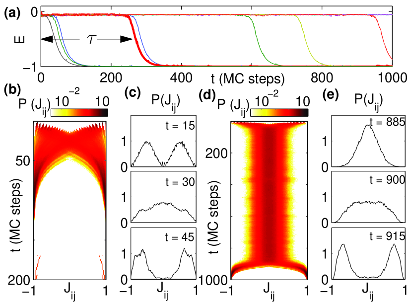
Figure 2: (a) Typical time-evolution of the energy per bond $E$ for a system of $N$ spins starting from different initial conditions. The relaxation time $\tau$ indicated in the figure is the duration after which $E$ decreases below $-0.5$. (b-e) Time-evolution of the distributions for the interaction strength $J_{ij}$ shown for two cases: (b-c) when the system relaxes rapidly and (d-e) when convergence takes much longer. Snapshots of the $J_{ij}$ distribution at specific times immediately before, during and immediately after the convergence are shown for the two cases in (c,e) respectively. For all figures $N=256$ with $T=51$, $\epsilon=0.05$.

Fig. 2 (a) shows the time-evolution of the order parameter $E$ for several typical runs for different initial conditions and realizations of a system with $T=15,\epsilon=0.05$. The order parameter of the system initially corresponds to that for a maximally disordered state ($\approx 0$) but eventually relaxes to a balanced state ($E=-1$). The time required for reaching balance, referred to as relaxation time, $\tau$, is estimated by measuring the duration starting from the initial state after which $E$ decreases below $-1/2$ [Fig. 2 (a)]. For a large range of parameters, we observe two very distinct types of behavior: in one, the system relaxes rapidly, while in the other this takes a longer time. In both cases, once the order parameter starts decreasing (i.e., after time $\tau$), it reaches a balanced state within a time-interval $\sim 1/\epsilon$. As this is typically much shorter than the relaxation time for the second case, the transition to the balanced state can appear rather suddenly for the latter. Before the onset of the convergence to the balanced state, the order parameter fluctuates over a very narrow range around zero, and there is little indication as to when the transition will happen. Characteristic time-evolution corresponding to these two types of behavior are shown in Fig. 2 (b-e). When the system relaxes rapidly, smaller peaks emerge from the two peaks of the initial $J_{ij}$ distribution (located at $\pm 1$) and eventually cross each other to reach the opposite ends asymptotically, converging to a two-peaked distribution again [Fig. 2 (b-c)], indicating that all interactions are now balanced. However, in the case where convergence takes significantly longer [Fig. 2 (d-e)], the initial distribution is first completely altered to a form resembling a Gaussian distribution with zero mean. After a long time, the system abruptly converges towards a balanced state with a corresponding transformation of the $J_{ij}$ distribution to one having peaks at $\pm 1$. Note that even with the same initial spin configuration and realization of $J_{ij}$ distribution, different MC runs generate distinct trajectories that are similar to those shown in Fig. 2 (a). This implies that knowledge of the initial conditions is not sufficient to decide whether the system will relax rapidly or not.

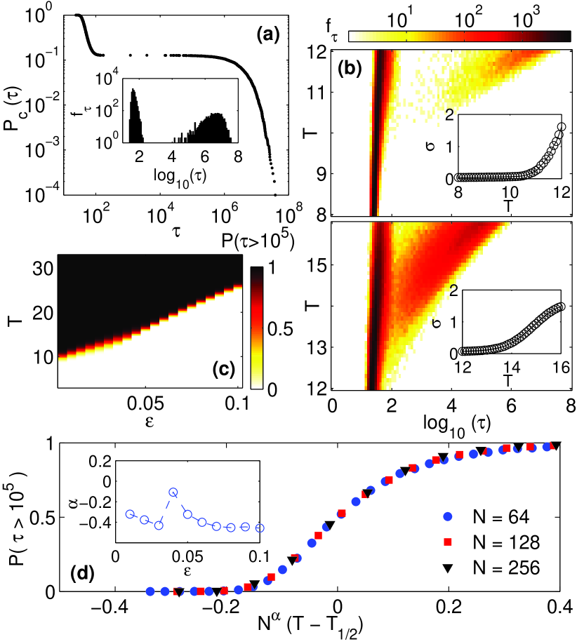
Figure 3: (a) The cumulative distribution of relaxation time $\tau$ for system of $N=64$ spins with $T=12,\epsilon=0.03$ shows a gap implying a bimodal nature for the distribution. The inset showing the corresponding frequency distribution $f_{\tau}$ for $\log_{10}(\tau)$ clearly indicates this bimodal nature. (b) Probability distributions of $\log_{10}(\tau)$ shown as a function of temperature $T$ for $\epsilon=0.03$ (top) and 0.05 (bottom) indicates the onset of bimodal behavior at higher values of temperature, e.g., for $T\gtrsim 10$ in (top). Bimodality appears around the temperature where the standard deviation of $\log_{10}(\tau)$ starts increasing appreciably from an almost constant value (insets). (c) The probability that relaxation takes longer than $10^{5}$ MC steps, $P(\tau>10^{5})$ shown as a function of $\epsilon$ and $T$. The point of transition from fast to slow convergence can be quantified by $T_{1/2}(\epsilon)$, i.e., the temperature at which $P(\tau>10^{5})$=1/2 for a given value $\epsilon$ (indicated by boundary between the dark and light regions). (d) Finite size scaling of the probability that relaxation takes longer than $10^{5}$ MC steps, $P(\tau>10^{5})$, with $N^{\alpha}(T-T_{1/2})$ for different system sizes $N$ ($\epsilon=0.05$). The temperature at which $P(\tau>10^{5})$ becomes half is represented as $T_{1/2}$. A scaling exponent value of $\alpha\approx-0.32$ shows reasonable data collapse. The inset shows the scaling exponents for the best data collapse at different values of $\epsilon$.

To quantitatively characterize the distinction between the two types of relaxation behavior, we focus on the statistics of $\tau$ (Fig. 3). Fig. 3 (a) shows the distribution of the relaxation time for a given set of $(T,\epsilon)$ where cases of both fast and slow convergences are seen. The resulting bimodal nature is clearly observed with the peak at lower $\tau$ ($\sim 100$ MC steps) corresponding to fast convergence to balanced state while that occurring at a higher value ($\sim 10^{7}$ MC steps) arises from the instances of slow relaxation. The distribution decays exponentially at very high values of $\tau$. Fig. 3 (b) shows the temperature dependence of the distribution of $\log_{10}(\tau)$ for two different values of $\epsilon$. For the smaller $\epsilon$ (= 0.03), the second peak is well-separated from the first when bimodality first appears, while for the larger $\epsilon$ (= 0.05) the second peak appears close to the first one. To estimate the temperature where the second peak appears, we plot the standard deviation of $\log_{10}(\tau)$ as a function of $T$ (inset), as bimodality is characterized by an increase in the dispersion of relaxation times. To observe how the distribution is affected by variation in both $T$ and $\epsilon$, we show in Fig. 3 (c) how the probability that the relaxation takes a long time (viz., $\geq 10^{5}$ MC steps) varies as a function of these two parameters. As we know that the system relaxes rapidly when the temperature is decreased close to zero, we expect this probability to be negligible at very low values of $T$. On the other hand, when temperature is increased to very high values, the relaxation takes increasingly longer, so that the probability $P(\tau>10^{5})$ approaches 1. We indeed observe a monotonic increase in this probability from 0 to 1 as the temperature is increased for a given value of $\epsilon$. We can define a transition temperature $T_{1/2}(\epsilon)$ as the value of $T$ at which this probability is equal to $1/2$. We observe that $T_{1/2}(\epsilon)$ increases with $\epsilon$, which implies that the relaxation to the balanced state requires a longer duration as the interaction dynamics becomes slower. For a given $\epsilon$, we study the variation of the probability $P(\tau>10^{5})$ with $T$ for different system sizes. Finite-size scaling shows data collapse with a scaling exponent $\alpha$ [Fig. 3 (d)] that varies with $\epsilon$ (inset). Depending on the value of $\epsilon$, we observe that there may be different types of bimodal distribution of the relaxation times, e.g., one where the second peak is clearly separated from the first, and the other where they are joined [Fig. 3 (b)]. The variation of $\alpha$ with $\epsilon$ appears to reflect this change from one type of bimodality to another (inset).

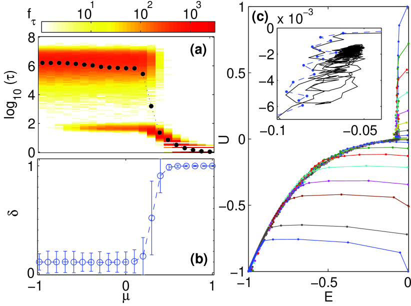
Figure 4: (a) Probability distribution of $\log_{10}(\tau)$ shown as a function of the mean $\mu$ of the initial distribution for $J_{ij}$ for $T=17$, $\epsilon=0.05$. The filled circles represent the average of $\log_{10}(\tau)$ for different values of $\mu$. The distribution does not change much for small bias ($|\mu|$); however the lower peak disappears as $\mu$ approached $-1$ while the the relaxation behavior occurs faster as $\mu$ approaches $+1$. (b) Scaled size difference $\delta=(C_{1}-C_{2})/N$ between the two clusters of aligned spins shown as a function of $\mu$. As $\mu$ increases from negative values to 1, $\delta$ increases from values close to 0 towards 1. (c) Trajectories representing the time-evolution of the system ($N=256$) in the ($E,U$) order parameter space for different values of $\mu$ (from top to bottom, $\mu$ increases from $-1$ to $1$ in steps of $0.1$). After transients, all trajectories converge to a single curve independent of the time required to converge to the balanced state. A magnified view (inset) compares the trajectory corresponding to a long relaxation time (solid curve), which appears to be trapped in this region, with the one corresponding to a short relaxation time (broken curve) for $\mu=0$.

So far we have assumed that the initial $J_{ij}$ distribution is unbiased (i.e., $\mu=0$). However, having a higher fraction of interactions of a particular sign can have significant consequences for both the structure of the final balanced state and the time required to converge to it. To investigate the role of this initial bias among the interaction strengths, we consider a distribution with two differently weighted $\delta$ function peaks at $\pm 1$ (i.e., $\mu\neq 0$). Fig. 4 (a) shows the distribution of the relaxation times as $\mu$ is varied over the interval [$-1,1$] with the parameters $T$, $\epsilon$ chosen such that there is a clear bimodal nature of the relaxation time distribution for the unbiased case ($\mu=0$). If all the interactions are anti-ferromagnetic ($\mu=-1$), the system is extremely frustrated and the relaxation to a balanced state may take a long time, whereas in the case where the interactions are all ferromagnetic ($\mu=1$), the system is balanced to begin with. Thus, with increasing $\mu$, we expect the relaxation time to decrease, which is indeed observed; in addition, the peak at higher values of $\tau$ disappears as $\mu$ approaches 1. On the other hand, when $\mu$ approaches $-1$, the peak corresponding to shorter relaxation times is no longer present. The two clusters that comprise the final balanced state can have very different size distributions depending on the bias in the initial distribution of $J_{ij}$. For the unbiased case, the two clusters are approximately of the same size. We observe from Fig. 4 (b) that this property holds for the entire range of negative values for $\mu$. As $\mu$ increases from 0, the size difference between the two clusters start increasing, eventually leading to a single cluster where all the spins interact with each other ferromagnetically ($\mu\simeq 1$). Note that if the system initially has a very low degree of frustration [e.g., $\mu\geq 0.4$ in Fig. 4 (a,b)], the system relaxes almost immediately to a balanced state where the larger cluster comprises almost the entire system. To visualize the coevolving dynamics in the link weights and spin orientations as the system approaches balance for different values of $\mu$, we use an additional order parameter Antal05 ; Marvel09 that measures the frustration in a signed network in terms of the fraction of triads deviating from balance (a triad being balanced if the product of its link weights approaches $+1$), $U=-\sum_{i,j,k}J_{ij}J_{jk}J_{ki}/{N\choose 3}$. Fig. 4 (c) shows that the trajectories corresponding to different values of $\mu$ converge to a single curve after transients, eventually reaching the balanced state at ($E=-1,U=-1$). For $\mu<0$, the initial trajectory is approximately vertical indicating that it is dominated by the adaptation dynamics (Eq. 2), whereas for $\mu>0$, it has strong horizontal component implying that it is governed primarily by the MC update of the spin states. Realizations in which the system takes a long time to relax to the balanced state are distinguished by trajectories that appear to be trapped in a confined region in the ($E,U$) space for a considerable period [Fig. 4 (c), inset].

We can qualitatively understand the appearance of short relaxation times as follows. In the initial state, when the system has a random assignment of interaction strengths, the energy landscape is extremely rugged, resembling that of a spin glass Fischer91 . The system starts out in a potential well corresponding to one of the many initially available local minima. As the state of the system evolves, the $J_{ij}$ dynamics (Eq. 2) lowers the energy of the state by making the interactions consistent with the spin orientations of the system, while the spin dynamics (updated according to the MC algorithm) can either result in a further lowering of energy as the state moves towards the bottom of the potential well, or is ejected from the initial local minima due to thermal fluctuations. The probability of escaping from the well at the $t$-th iteration, $p(t)$, depends on the potential barrier height with neighboring wells. If the state cannot escape in the first few iterations from the local minimum from which it starts, successive lowering of the energy of this well by the $J_{ij}$ dynamics results in the minima becoming deeper, so that the probability of escape is reduced further. Eventually, the system relaxes to the balances state with a time-scale of $\sim\epsilon^{-1}$, when the well becomes the global minimum of a smooth energy landscape. On the other hand, if the state escapes from the initial well within the first few iterations, when the $J_{ij}$ dynamics has not yet been able to significantly reduce the energy of a particular well, the barrier heights separating the different local minima are all relatively low. As a result, the system can jump from one well to another with ease, corresponding to frequent switching of the spin orientations. As $J_{ij}$ moves towards $\sigma_{i}\sigma_{j}$ at any given time (Eq. 2), rapid changes in the sign of the latter implies that there is effectively no net movement of $J_{ij}$ towards $\pm 1$. In fact, in this case, we observe that the initial distribution of $J_{ij}$, comprising delta-function peaks at $\pm 1$, transforms within a few iterations to one resembling a Gaussian peaked at zero [Fig. 2 (d-e)]. Once the system reaches such a state, it can only attain a balanced state through a low-probability event which corresponds to the state remaining in the same local minimum for several successive time steps. As such an event will only happen after extremely long time, this will lead to a very large relaxation time for a range of $T$ and $\epsilon$. Let us assume for simplicity that when the system is in the state corresponding to frequent spin flips and low interaction strengths, the probability of escaping from a local minimum is approximately a constant ($p(t)\approx p$). Then the probability that the system jumps between different minima for $t$ steps and gets trapped in the $t+1$-th step is $p^{t}(1-p)$. This results in the distribution of the relaxation times (under the simplifying assumption of constant $p$) having an exponential tail, which is indeed observed [Fig. 3 (a)].

To conclude, we have shown that a link adaptation dynamics inspired by the Hebbian principle can result in an initially frustrated network achieving structural balance. However, in the presence of fluctuations, we observe that the system exhibits a large dispersion in the time-scale of relaxation to the balanced state, characterized by a bimodal distribution. This extreme variability of the time required to converge to the balanced state is a novel phenomenon that requires further investigation. Our result suggests that even when a system has the potential of attaining structural balance, the time required for this process to converge may be so large that it will not be observed in practice. Although we have considered a globally connected network of binary state dynamical elements, it is possible to extend our analysis to sparse networks Dasgupta09 and different kinds of nodal dynamics (e.g., $q$-state Potts model). As many networks seen in nature have directed links, a generalization of the concept of balance to directed networks and understanding how it can arise may provide important insights on the evolution of such systems.

We thank Chandan Dasgupta, Deepak Dhar, S. S. Manna, Shakti N. Menon and Purusattam Ray for helpful discussions. This work was supported in part by CSIR, UGC-UPE, IMSc Associate Program and IMSc Complex Systems Project. We thank IMSc for providing access to the “Annapurna” supercomputer.

References

- (1) M. E. J. Newman, Networks: An Introduction (Oxford Univ. Press, Oxford, 2010).
- (2) A. Barrat, M. Barthélemy and A. Vespignani, Dynamical Processes on Complex Networks (Cambridge Univ. Press, Cambridge, 2008).
- (3) S. N. Dorogovtsev, A. V. Goltsev and J. F. F. Mendes, Rev. Mod. Phys. 80, 1275 (2008).
- (4) S. Jain and S. Krishna, Proc. Natl. Acad. Sci. USA 98, 543 (2001).
- (5) T. Gross, C. J. D. D’Lima and B. Blasius, Phys. Rev. Lett. 96, 208701 (2006); T. Gross and B. Blasius, J. Roy. Soc. Interface 5, 259 (2008).
- (6) B. D. MacArthur, R. J. Sánchez-García and A. Ma’ayan, Phys. Rev. Lett. 104, 168701 (2010).
- (7) R. Durrett et al., Proc. Natl. Acad. Sci. USA 109, 3682 (2012).
- (8) A. Goudarzi, C. Teuscher, N. Gulbahce and T. Rohlf, Phys. Rev. Lett. 108, 128702 (2012).
- (9) W. Liu, B. Schmittmann and R. K. P. Zia, EPL 100, 66007 (2012).
- (10) A. Barrat, M. Barthélemy, R. Pastor-Satorras and A. Vespignani, Proc. Natl. Acad. Sci. USA 101, 3747 (2004); A. Barrat, M. Barthélemy and A. Vespignani, Phys. Rev. Lett. 92, 228701 (2004).
- (11) J.-P. Onnela et al., Proc. Natl. Acad. Sci. USA 104, 7332 (2007).
- (12) V. A. Traag and J. Bruggeman, Phys. Rev. E 80, 036115 (2009).
- (13) K. H. Fischer and J. A. Hertz, Spin Glasses (Cambridge Univ. Press, Cambridge, 1991); M. Mezard, G. Parisi, M. A. Virasoro, Spin Glass Theory and Beyond (World Scientific, Singapore, 1987).
- (14) F. Heider, J. Psychol. 21, 107 (1946).
- (15) D. Cartwright and F. Harary, Psychol. Rev. 63, 277 (1956).
- (16) R. Singh, S. Dasgupta and S. Sinha, EPL 95, 10004 (2011).
- (17) T. Antal, P. L. Krapivsky and S. Redner, Phys. Rev. E 72, 036121 (2005).
- (18) S. A. Marvel, S. H. Strogatz and J. M. Kleinberg, Phys. Rev. Lett. 103 198701 (2009).
- (19) K. Kułakowski, P. Gawronski and P. Gronek, Int. J. Mod. Phys. C 16 707 (2005).
- (20) S. A. Marvel, J. Kleinberg, R. D. Kleinberg and S. H. Strogatz, Proc. Natl. Acad. Sci. USA 108, 1771 (2011); T. H. Summers and I. Shames, EPL 103 18001 (2013).
- (21) M. D. Fox et al. Proc. Natl. Acad. Sci. USA 102, 9673 (2005).
- (22) D. O. Hebb, The Organization of Behavior (Wiley, New York, 1949); B. L. McNaughton, Phil. Trans. R. Soc. B 358, 629 (2003).
- (23) C. T. Fernando et al., J. R. Soc. Interface 6, 463 (2009); R. A. Watson, C. L. Buckley, R. Mills and A. Davies, in Artificial Life XII, edited by H. Fellermann et al. (MIT Press, Cambridge, 2010), p. 194.
- (24) G. Facchetti, G. Iacono and C. Altafini, Proc. Natl. Acad. Sci. USA 108, 20953 (2011); Phys. Rev. E 86, 036116 (2012).
- (25) S. Dasgupta, R. K. Pan and S. Sinha, Phys. Rev. E 80, 025101 (2009); R. K. Pan and S. Sinha, EPL 85, 68006 (2009).