On the existence of moments for high dimensional importance sampling

Abstract

Theoretical results for importance sampling rely on the existence of certain moments of the importance weights, which are the ratios between the proposal and target densities. In particular, a finite variance ensures square root convergence and asymptotic normality of the importance sampling estimate, and can be important for the reliability of the method in practice. We derive conditions for the existence of any required moments of the weights for Gaussian proposals and show that these conditions are almost necessary and sufficient for a wide range of models with latent Gaussian components. Important examples are time series and panel data models with measurement densities which belong to the exponential family. We introduce practical and simple methods for checking and imposing the conditions for the existence of the desired moments. We develop a two component mixture proposal that allows us to flexibly adapt a given proposal density into a robust importance density. These methods are illustrated on a wide range of models including generalized linear mixed models, non-Gaussian nonlinear state space models and panel data models with autoregressive random effects.

Keywords: MCMC, simulated maximum likelihood, state space models, robustness

1 Introduction

This paper develops robust high-dimensional importance sampling methods for estimating the likelihood of statistical and econometric models with latent Gaussian variables. We propose computationally practical methods for checking and ensuring that the second (and possibly higher) moments of the importance weights are finite. The existence of particular moments of the importance weights is fundamental for establishing the theoretical properties of estimators based on importance sampling. A central limit theorem applies to the importance sampling estimator if the second moment of the weights is finite (Geweke,, 1989). The Berry-Esseen theorem (Berry,, 1941; Esseen,, 1942) specifies the rate of convergence to normality when the third moment exists. In a more general case where the weights can have local dependence and may not be identically distributed, if the $n^{\text{th}}$ moment of the weights exists, Chen and Shao, (2004) show that the rate of convergence to normality is of the order of $O(S^{-(n-2)/4})$ with $S$ the number of importance samples. This implies that the higher the moments that exist, the faster the rate of convergence. Even though infinite variance may in some cases be due to a region of the sampling space that has no practical impact for Monte Carlo sampling (Owen and Zhou,, 2001), this problem can result in highly inaccurate importance sampling estimates in a variety of applications; see Robert and Casella, (2005) and Richard and Zhang, (2007) for examples.

In many models, e.g. non-Gaussian nonlinear state space models and generalized linear mixed models, the likelihood involves analytically intractable integrals. These integrals are often estimated by importance sampling. A popular approach for estimating the parameters in such models is the simulated maximum likelihood (SML) method (see, e.g., Gourieroux and Monfort,, 1995). SML first estimates the likelihood by importance sampling and then maximizes the estimated likelihood. A second approach for estimating such models is by Bayesian inference using Markov chain Monte Carlo simulation. If the likelihood is estimated unbiasedly, then the Metropolis-Hastings algorithm with the likelihood replaced by its unbiased estimator is still able to sample exactly from the posterior. See, for example, Andrieu and Roberts, (2009) and Flury and Shephard, (2011). Pitt et al., (2012) show that it is crucial for this approach that the variance of the estimator of the log-likelihood exists, which is guaranteed by a finite second moment of the weights when the likelihood is estimated by importance sampling. Both the SML and MCMC methods require an efficient importance sampling estimator of the likelihood.

This paper introduces methods that directly check the existence of any particular moment of the importance weights when using a possibly high-dimensional Gaussian importance density. If the Gaussian importance density does not possess the required moments, our results make it straightforward to modify the original Gaussian importance density in such a way that the desired moment conditions hold. This approach is extended by developing a mixture importance density which is a combination of that robust modified Gaussian density with any other importance density. We prove that this mixture importance density satisfies the desired moment conditions, while providing substantial flexibility to design practical and efficient importance densities. The only requirement for the validity of these methods is that the log measurement density is concave or bounded linearly from above as a function of the latent variables. Our method contrasts with previous approaches which rely on statistical testing. See for example Monahan, (1993) and Koopman et al., (2009), who develop diagnostic tests for infinite variance based on extreme value theory.

We also develop specific results that allow us to efficiently check and impose the required moment conditions for nonlinear non-Gaussian state space models. Gaussian importance samplers are extensively applied in this setting. Some examples include non-Gaussian unobserved components time series models as in Durbin and Koopman, (2000), stochastic volatility models in Liesenfeld and Richard, (2003), stochastic conditional intensity models in Bauwens and Hautsch, (2006), stochastic conditional duration models in Bauwens and Galli, (2009), stochastic copula models in Hafner and Manner, (2012) and dynamic factor models for multivariate counts in Jung et al., (2011).

We illustrate the new method in a simulation study and in an empirical application to Bayesian inference for a Poisson panel data model with autoregressive random effects. We consider the Shephard and Pitt, (1997) and Durbin and Koopman, (1997) (SPDK) importance sampling algorithm, a commonly used approach based on local approximation techniques. We find that the SPDK method leads to infinite variance for this problem. The results show that the mixture approach for imposing the finite variance condition can provide an insurance against poor behavior of the SPDK method for estimating the likelihood at certain parameter values (for example, at the tail of the posterior density), even though the standard method performs nearly as well in most settings. This result suggests that the infinite variance problem typically has low probability of causing instability for this example. We also show that the mixture importance sampler leads to more efficient estimates compared to Student’s $t$ importance sampler with the same mean and covariance matrix as the SPDK Gaussian sampler.

Section 2 provides the background to importance sampling and establishes the notation. Section 3 presents the main theoretical results. Section 4 discusses the robust importance sampling methods for three popular classes of models including generalized linear mixed models, non-Gaussian nonlinear state space models and panel data models. Section 5 provides several illustrative examples.

2 Importance sampling

In many statistical applications we need to estimate an analytically intractable likelihood of the form

$$L(\psi)=\int p(y|\alpha;\psi)p(\alpha;\psi)d\alpha,$$ (1)

where $y$ is the observed data, $\alpha$ is a $d\times 1$ vector of latent variables, and $\psi$ is a fixed parameter vector at which the likelihood is evaluated. The density $p(y|\alpha;\psi)$ is the conditional density of the data given the latent variable $\alpha$ and $p(\alpha;\psi)$ is the density of $\alpha$. These densities usually depend on a parameter vector $\psi$. In some classes of models such as state space models, (1) can be a very high-dimensional integral. In some other classes such as generalized linear mixed models and panel data models, the likelihood decomposes into a product of lower dimensional integrals. Since the parameter vector $\psi$ has no impact on the mathematical arguments that follow, we omit to show this dependence, except that we still write $L(\psi)$ to explicitly indicate the dependence of the likelihood on $\psi$.

To evaluate the integral (1) by importance sampling, we write it as

$$L(\psi)=\int\frac{p(y|\alpha)p(\alpha)}{g(\alpha)}g(\alpha)\,\textrm{d}\alpha=\int\omega(\alpha)g(\alpha)\,\textrm{d}\alpha,$$

where $g(\alpha)$ is an importance density whose support contains the support of $p(y|\alpha)p(\alpha)$, and $\omega(\alpha)={p(y|\alpha)p(\alpha)}/{g(\alpha)}$ is the importance weight. Let $\alpha_{1},\ldots,\alpha_{S}$ be $S$ draws from the importance density $g(\alpha)$. Then the likelihood (1) is estimated by $\widehat{L}(\psi)=\frac{1}{S}\sum_{s=1}^{S}\omega(\alpha_{s})$. Let

$$E_{g}[\omega(\alpha)^{n}]=\int\omega(\alpha)^{n}g(\alpha)d\alpha.$$ (2)

If $E_{g}[\omega(\alpha)]<\infty$, a strong law of large numbers holds, i.e. $\widehat{L}(\psi)\stackrel{{\scriptstyle a.s.}}{{\longrightarrow}}L(\psi)$ as $S\rightarrow\infty$. Let $W=\sqrt{S}(\widehat{L}-L)/\sigma_{w}$ where $\sigma^{2}_{w}=\text{\rm Var}_{g}(w(\alpha))$. If $E_{g}[\omega(\alpha)^{2}]<\infty$, a central limit theorem holds, i.e. $W\stackrel{{\scriptstyle d}}{{\to}}N(0,1)$ (see, e.g., Geweke,, 1989). Furthermore, if $E_{g}[\omega(\alpha)^{3}]<\infty$, the rate of convergence of $\widehat{L}$ to normality can be determined by the Berry-Esseen theorem (Berry,, 1941; Esseen,, 1942), which states that

$$\sup_{z}|P(W\leq z)-\Phi(z)|\leq\frac{1}{\sqrt{S}}C\gamma,$$

where $\gamma=E_{g}[|\omega(\alpha)-L|^{3}]$, $C$ is a finite constant and $\Phi(z)$ is the standard normal cdf.

Our article first obtains conditions for the existence of the required moments of the weights $\omega(\alpha)$ when using a Gaussian importance density $g(\alpha)=\textrm{\rm N}(\alpha|\mu^{\ast},Q^{\ast-1})$. The results are then extended to the case of a mixture importance density.

3 General properties of importance weights

We are concerned with the existence of the $n^{th}$ moment $E_{g}[\omega(\alpha)^{n}]$ of the importance weights $\omega(\alpha)$ when using a Gaussian importance density $g(\alpha)=\textrm{\rm N}(\alpha|\mu^{\ast},Q^{\ast-1})$. In this paper, $n$ can be any positive number. Of special interest is cases where $n$ is a positive integer and we refer to $n=1$ as the fist moment, $n=2$ as the second moment and so forth. Let $l(\alpha)=\log p(y|\alpha)$. We write the log of the importance weights as

$$\log\omega(\alpha) =l(\alpha)+\log p(\alpha)-\log g(\alpha)$$

$$=c+l(\alpha)+\log p(\alpha)+\frac{1}{2}(\alpha-\mu^{\ast})^{\prime}Q^{\ast}(\alpha-\mu^{\ast}),$$

where the constant $c$ does not depend on $\alpha$. In this paper, for a square matrix $A$, the notation $A>0$ ($A<0$) means that $A$ is a positive definite (negative definite). We obtain the following general result on the moments of $\omega(\alpha)$.

Proposition 1.

Suppose that there exists a constant scalar $k$, a vector $\xi$ and a symmetric matrix $Q>0$ such that

$$l(\alpha)+\log p(\alpha)\leq k-\frac{1}{2}(\alpha-\xi)^{\prime}Q(\alpha-\xi),\text{ for all }\alpha.$$ (3)

Then $E_{g}[\omega(\alpha)^{m}]<\infty$ for all $m\leq n$ if $Q^{*}$ satisfies

$$Q^{\ast}-n(Q^{\ast}-Q)>0.$$ (4)

Proof.

See Appendix A. ∎

When $n=0$ condition (4) requires that the inverse covariance matrix $Q^{\ast}$ of the importance density $g(\alpha)$ is positive definite. For $n=1$, condition (4) holds because $Q>0$ by assumption. The requirement for a finite variance of the weights, corresponding to the case $n=2$, requires that $2Q-Q^{\ast}>0$. In practice the bounding assumption (3) can be difficult to verify for general models. However, for models in which the density of the latent vector $p(\alpha)$ is Gaussian, verifying this assumption is straightforward. Also, when $p(\alpha)$ is Gaussian it is relatively straightforward to check the existence condition (4) and to impose conditions on $Q^{*}$ to ensure the existence of specific moments of the weights. The rest of this paper will therefore focus on models for which the latent density $p(\alpha)$ is itself multivariate Gaussian $N(\alpha|\mu,Q^{-1})$ with $Q>0$.

Proposition 2.

(i) Suppose that there exists a constant scalar $k$, and a vector $\delta$ such that

$$l(\alpha)=\log p(y|\alpha)\leq k+\delta^{\prime}\alpha,\text{ for all }\alpha.$$ (5)

Then $E_{g}[\omega(\alpha)^{m}]<\infty$ for all $m\leq n$ if $Q^{\ast}-n(Q^{\ast}-Q)>0$.

(ii) Suppose that for at least one $j$ ($j=1,...,d$),

$$\text{either}\;\;\lim_{\alpha_{j}\to-\infty}\frac{l(\alpha)}{\alpha_{j}^{2}}=0\;\;\text{or}\;\;\lim_{\alpha_{j}\to+\infty}\frac{l(\alpha)}{\alpha_{j}^{2}}=0.$$ (6)

Then $Q^{\ast}-n(Q^{\ast}-Q)<0$ implies $E_{g}[\omega(\alpha)^{n}]=\infty$.

Proof.

See Appendix A. ∎

Part (i) of Proposition 2 indicates that when the log measurement density is concave in the latent variable $\alpha$, a sufficient condition for the existence of the first $n$ moments is that $Q^{\ast}-n(Q^{\ast}-Q)>0$. Under the additional assumption of part (ii), the condition is also necessary. For many models, it is possible to verify these Assumptions. Assumption (5) covers all exponential family models with a canonical link to the latent variable $\alpha$, i.e. the density $p(y|\alpha)$ is of the form

$$p(y|\alpha)=\exp\left(\frac{y\eta(\alpha)-b(\eta(\alpha))}{\varpi}\right),$$

where $\eta(\alpha)=z^{\prime}\alpha+c$, $z$ is a vector of covariates, $c$ is a constant that does not depend on $\alpha$, and $\varpi>0$ is a dispersion parameter (see Section 4). Because $\ddot{b}(\eta)=\partial^{2}b(\eta)/\partial\eta^{2}>0$ by the property of the exponential family,

$$\frac{\partial^{2}l(\alpha)}{\partial\alpha\partial\alpha^{T}}=-\frac{1}{\varpi}\ddot{b}(\eta(\alpha))zz^{\prime}<0.$$

It follows that $l(\alpha)$ is a concave function in $\alpha$, because a differentiable function is concave if and only if its Hessian matrix is negative definite (see, e.g., Bazaraa et al.,, 2006, Chapter 3). Similarly, we can show that the stochastic volatility model (see, e.g., Ghysels et al.,, 1996) satisfies (5) with Gaussian or Student $t$ errors in the observation equation. The observation equation for the univariate stochastic volatility model with Gaussian errors is $y_{t}=\exp(\alpha_{t}/2)\epsilon_{t}$, $t=1,...,T$, with $\epsilon_{t}\sim N(0,1)$. Hence,

$$l(\alpha)=-\frac{T}{2}\log(2\pi)-\frac{1}{2}\sum_{t=1}^{T}\alpha_{t}-\frac{1}{2}\sum_{t=1}^{T}y_{t}^{2}\exp(-\alpha_{t}),\;\;\alpha=(\alpha_{1},...,\alpha_{T})^{\prime}.$$ (7)

It is straightforward to show that the Hessian matrix of $l(\alpha)$ is negative definite, thus $l(\alpha)$ is concave. The concavity of $l(\alpha)$ in the case with $t$ errors can be shown similarly.

Assumption (6) is also satisfied by many popular models. For example, in the Poisson model where $b(\eta(\alpha))=\exp(z^{\prime}\alpha+c)$ and in the binomial model where $b(\eta(\alpha))=\log(1+e^{z^{\prime}\alpha+c})$, we can easily check that (6) holds. For the stochastic volatility model with $l(\alpha)$ given in (7), (6) holds because $\lim_{\alpha_{j}\to+\infty}(l(\alpha)/\alpha_{j}^{2})=0$ for any $j$.

3.1 A general method for checking and imposing the existence condition

This section presents a general method for checking and imposing the existence condition (4). A more efficient method that exploits the structure of non-Gaussian nonlinear state space models is presented in Section 4.2.

Suppose that $g(\alpha)=\textrm{\rm N}(\alpha|\mu^{\ast},Q^{\ast-1})$ is an importance density available in the literature, e.g. one obtained by the Laplace method. It is straightforward to check the positive definiteness of the matrix $Q^{\ast}-n(Q^{\ast}-Q)$ by verifying that all its eigenvalues are positive or by using Sylvester’s criterion, which is discussed in Section 4.2.1.

If $Q^{*}$ fails the existence condition, we modify $Q^{*}$ to construct a matrix $\widetilde{Q}$ such that $\widetilde{Q}-n(\widetilde{Q}-Q)>0$ by first decomposing $nQ=AA^{\prime}$ using the Cholesky decomposition. Let $V$ be the diagonalization matrix of $A^{-1}Q^{*}{A^{\prime}}^{-1}$, i.e. $V^{\prime}A^{-1}Q^{*}{A^{\prime}}^{-1}V=\Lambda$, where $\Lambda=\text{diag}(\lambda_{1},...,\lambda_{d})$ is a diagonal matrix, $VV^{\prime}=V^{\prime}V=I$. Such an orthonormal matrix $V$ always exists as $A^{-1}Q^{*}{A^{\prime}}^{-1}$ is real and symmetric. We define $\widetilde{\Lambda}=\text{diag}(\widetilde{\lambda}_{1},...,\widetilde{\lambda}_{d})$ with

$$\widetilde{\lambda}_{j}=\begin{cases}\lambda_{j},&\text{if}\;\;\lambda_{j}<1/(n-1),\\ \frac{1-\epsilon}{n-1},&\text{if}\;\;\lambda_{j}\geq 1/(n-1).\end{cases}$$ (8)

for some $\epsilon>0$. Note that $\widetilde{\lambda}_{j}<1/(n-1)$ for all $j=1,...,d$. Finally, let $\widetilde{Q}=AV\widetilde{\Lambda}V^{\prime}A^{\prime}$. It follows that $nQ-(n-1)\widetilde{Q}=AV(I-(n-1)\widetilde{\Lambda})V^{\prime}A^{\prime}>0$. The new importance density $\widetilde{g}(\alpha)=\textrm{\rm N}(\alpha|\mu^{\ast},\widetilde{Q}^{-1})$ then satisfies the existence condition (4).

For SML, it is essential that the likelihood estimator $\widehat{L}(\psi)$ is continuous, and desirably, differentiable with respect to the model parameters $\psi$. The function $\widetilde{\lambda}_{j}=\widetilde{\lambda}_{j}(\lambda_{j})$ in (8) is not a continuous function of $\lambda_{j}$, so $\widetilde{\lambda}_{j}(\psi)=\widetilde{\lambda}_{j}(\lambda_{j}(\psi))$ is not continuous in $\psi$. Appendix C presents a modification of (8) in which $\widetilde{\lambda}_{j}$ is a continuous and differentiable function of $\lambda_{j}$.

The principle behind the above method is that the difference $\widetilde{Q}-Q^{*}$ is often small, so that $\widetilde{g}(\alpha)$ still provides a good fit to the target density, while the condition for the existence of the $n^{th}$ moment is guaranteed to hold. Intuitively, only directions of $Q^{\ast}$ along which the density $N(\alpha|\mu^{*},{Q^{*}}^{-1})$ has light tails are modified; the other directions are unchanged. The resulting density $N(\alpha|\mu^{*},{\widetilde{Q}}^{-1})$ has heavier tails than the original density $N(\alpha|\mu^{*},{Q^{*}}^{-1})$.

However, we have seen that the observation density $p(y|\alpha)$ does not matter for the existence of moments under the assumptions of Proposition 2, so that the importance density $\widetilde{g}(\alpha)$ may be a poor approximation to $p(y|\alpha)p(\alpha)$ near its mode. To overcome this problem, we establish the following result. Let $f(\alpha)=p(y|\alpha)p(\alpha)$ and $\sup(f)=\{\alpha:f(\alpha)\not=0\}$ be the support of $f$.

Proposition 3.

Suppose that $g_{1}(\alpha)$ is a density such that $\sup(g_{1})\supseteq\sup(f)$, and for some $n\geq 0$,

$$\int_{\sup(g_{1})}\left(\frac{f(\alpha)}{g_{1}(\alpha)}\right)^{n}g_{1}(\alpha)d\alpha<\infty.$$ (9)

For any density $g_{2}(\alpha)$, consider the mixture importance density $g(\alpha)=\pi g_{1}(\alpha)+(1-\pi)g_{2}(\alpha)$ with $0<\pi<1$. Then, for all $m\leq n$,

$$\int_{\sup(g)}\left(\frac{f(\alpha)}{g(\alpha)}\right)^{m}g(\alpha)d\alpha<\infty.$$

Proof.

See Appendix A. ∎

The proposition suggests an approach to combine the importance density provided by the standard methods with a second importance density which by itself ensures the existence of the required moments. This result gives substantial flexibility in that it is useful in practice to put very little weight on the heavy density component $g_{1}(\alpha)$, while leaving the rest of the mass for the lighter tailed component. The existence of the moments will still be entirely governed by the heavier term $g_{1}(\alpha)$, but the use of the mixture proposal may lead to lower variance since $g_{2}(\alpha)$ is designed to approximate the target density accurately.

In all the models and examples considered in this article, Assumption (9) is satisfied with $g_{1}(\alpha)=N(\alpha|\mu^{*},{\widetilde{Q}}^{-1})$ and it is obvious that $\sup(g_{1})\supseteq\sup(f)$ as $\sup(g_{1})=\mathbb{R}^{d}$. The density $g_{2}(\alpha)$ can be any density that we can sample from. In practice, we would like to choose $g_{2}$ such that the weight $\omega(\alpha)$ has a small variance, while the desired moments are theoretically guaranteed to exist. In this paper we choose $g_{2}(\alpha)=N(\alpha|\mu^{*},{Q^{*}}^{-1})$, and set $\pi=0.1$ based on some experimentation. We refer to this approach as the $n^{\text{th}}$-moment constrained mixture importance sampler or $n^{\text{th}}$-IS for short.

4 Models

4.1 Generalized linear mixed models

A popular class of models that typically needs importance sampling for likelihood estimation is generalized linear mixed models (GLMM) (see, e.g., Jiang,, 2007). Consider a GLMM with data $y_{i}=(y_{i1},...,y_{in_{i}})^{\prime}$, $i=1,...,m$. Conditional on the random effects $\alpha_{i}$, the observations $y_{ij}$ are independently and exponentially distributed as

$$p(y_{ij}|\beta,\alpha_{i})=\exp\left(\frac{y_{ij}\eta_{ij}-b(\eta_{ij})}{\varpi}+c(y_{ij},\varpi)\right),$$

with $\eta_{ij}=x_{ij}^{\prime}\beta+z_{ij}^{\prime}\alpha_{i},\ j=1,...,n_{i},\ i=1,...,m,$ where $x_{ij},\ z_{ij}$ are $p$- and $u$-vectors of covariates. For simplicity, we assume that the dispersion parameter $\varpi$ is known; the cases with an unknown $\varpi$ require only a small modification to the procedure described below. The random effects are assumed to have a normal distribution $\alpha_{i}\stackrel{{\scriptstyle iid}}{{\sim}}N(0,Q^{-1})$. The parameters of interest are $\psi=(\beta,Q)$. The density of $y$ conditional on $\psi$ and $\alpha$ is

$$p(y|\psi,\alpha)=\prod_{i=1}^{m}p(y_{i}|\beta,\alpha_{i})=\prod_{i=1}^{m}\prod_{j=1}^{n_{i}}p(y_{ij}|\beta,\alpha_{i}),$$

so that the likelihood is

$$L(\psi)=p(y|\psi)=\prod_{i=1}^{m}L_{i}(\psi)\;\;\text{with}\;\;L_{i}(\psi)=\int p(y_{i}|\beta,\alpha_{i})p(\alpha_{i}|Q)d\alpha_{i}.$$ (10)

It is often difficult to estimate the model parameters $\psi$ because the likelihood (10) involves analytically intractable integrals $L_{i}(\psi)$. A popular approach for estimating $\psi$ is the SML method (see, e.g., Gourieroux and Monfort,, 1995). SML first estimates the integrals in (10) by importance sampling and then maximizes the estimated likelihood over $\psi$. It is necessary to use common random numbers so that the resulting estimator $\widehat{L}(\psi)$ is smooth in $\psi$. Another approach for estimating $\psi$ is by using MCMC with the likelihood (10) replaced by its unbiased estimator (Andrieu and Roberts,, 2009; Flury and Shephard,, 2011; Pitt et al.,, 2012).

Both the SML and MCMC methods require an efficient estimator of the likelihood (10). The robust importance sampling approach for estimating the integrals $L_{i}(\psi)$ can be carried out as follows. Write $X_{i}=[x_{i1},...,x_{in_{i}}]^{\prime}$, $Z_{i}=[z_{i1},...,z_{in_{i}}]^{\prime}$, $\eta_{i}=X_{i}\beta+Z_{i}\alpha_{i}$. Let $F_{i}(\alpha_{i})=\log p(y_{i}|\beta,\alpha_{i})+\log p(\alpha_{i}|Q)$, then

$$F_{i}(\alpha_{i})=\varpi^{-1}\left(y_{i}^{\prime}X_{i}\beta+y_{i}^{\prime}Z_{i}\alpha_{i}-\mathbf{1}_{n_{i}}^{\prime}b(\eta_{i})\right)-\frac{1}{2}\alpha_{i}^{\prime}Q\alpha_{i}+C,$$

where $C$ is the constant term independent of $\alpha_{i}$. Then

$$\frac{\partial F_{i}(\alpha_{i})}{\partial\alpha_{i}}=\varpi^{-1}\left(Z_{i}^{\prime}y_{i}-Z_{i}^{\prime}\dot{b}(\eta_{i})\right)-Q\alpha_{i}$$

and

$$H_{i}(\alpha_{i})=\frac{\partial^{2}F_{i}(\alpha_{i})}{\partial\alpha_{i}\partial\alpha_{i}^{\prime}}=-\varpi^{-1}Z_{i}^{\prime}\text{diag}(\ddot{b}(\eta_{i}))Z_{i}-Q,$$

where $\dot{b}(\eta)$ and $\ddot{b}(\eta)$ are the first and second derivatives of $b(\eta)$ and are understood componentwise, i.e. $\dot{b}(\eta)=(\dot{b}(\eta_{1}),...,\dot{b}(\eta_{k}))^{\prime}$, $\ddot{b}(\eta)=(\ddot{b}(\eta_{1}),...,\ddot{b}(\eta_{k}))^{\prime}$ when $\eta=(\eta_{1},...,\eta_{k})^{\prime}$ is a vector. It is straightforward to use Newton’s method to find a maximizer $\alpha_{i}^{*}$ of $F_{i}(\alpha_{i})$, because both the first and second derivatives of $F_{i}(\alpha_{i})$ are available in closed form. Let $Q_{i}^{*}=-H_{i}(\alpha_{i}^{*})$. We can now construct the $n^{\text{th}}$-moment constrained mixture importance sampler as described in Section 3.1 to ensure the existence of the first $n$ moments of the weights. It is therefore straightforward to carry out importance sampling in GLMM with the required moments of the weights guaranteed to exist. We note that $l_{i}(\alpha_{i})=\log p(y_{i}|\beta,\alpha_{i})$ is concave in $\alpha_{i}$ for all GLMMs with the canonical link (see Section 3), so that Proposition 2(i) applies.

A common practice is to use a $t$ importance density with mean $\alpha^{*}_{i}$, scale matrix ${Q^{*}_{i}}^{-1}$ and small degrees of freedom $\nu$, although the moments of the weights are not theoretically guaranteed to exist. Section 5.4 compares empirically the performance of such a $t$ importance density to our constrained mixture importance density.

4.2 Nonlinear non-Gaussian state space models

Consider the following class of nonlinear non-Gaussian state space models

$$\begin{split}y_{t}|\theta_{t}\sim p(y_{t}|\theta_{t};\psi),\qquad&\theta_{t}=c_{t}+Z_{t}\alpha_{t},\qquad t=1,\ldots,T,\\ \alpha_{t+1}=d+\Phi\alpha_{t}+\eta_{t},\qquad&\alpha_{1}\sim\textrm{\rm N}(\mu,\Sigma_{\alpha}),\qquad\eta_{t}\sim\textrm{\rm N}(0,\Sigma),\end{split}$$ (11)

where $y_{t}$ is the $k\times 1$ observation vector, $\theta_{t}$ is the $p\times 1$ signal vector, $\alpha_{t}$ is the $m\times 1$ state vector, and $Z_{t}$ is the $p\times m$ selection matrix; the $m\times 1$ constant vector $d$, the $m\times m$ transition matrix $\Phi$ and the $m\times m$ covariance variance matrix $\Sigma$ jointly determine the dynamic properties of the model. The parameter vector $\psi$ contains the unknown coefficients in the observation density and in the system matrices. A thorough overview of the models and methodology is provided in Durbin and Koopman, (2001).

Define $\alpha=(\alpha_{1}^{\prime}\,,\,\ldots\,,\,\alpha_{T}^{\prime})^{\prime}$ and $y=(y_{1}^{\prime}\,,\,\ldots\,,\,y_{T}^{\prime})^{\prime}$. The likelihood for the model is

$$L(\psi)=\int p(y|\alpha)p(\alpha)\,\textrm{d}\alpha=\int\prod_{t=1}^{T}p(y_{t}|\alpha_{t})p(\alpha_{1})\prod_{t=2}^{T}p(\alpha_{t}|\alpha_{t-1})\,\textrm{d}\alpha_{1}\ldots\,\textrm{d}\alpha_{T},$$ (12)

with $p(\alpha)=p(\alpha_{1})\prod_{t=2}^{T}p(\alpha_{t}|\alpha_{t-1})$ and $p(y|\alpha)=\prod_{t=1}^{T}p(y_{t}|\alpha_{t})$. The latent states are Gaussian, with $p(\alpha)=N(\alpha|\mu;Q^{-1})$, where $Q$ is a block tridiagonal matrix because the states $\alpha_{t}$ follow a first order autoregressive process. A closed form representation of $Q$ is derived in Appendix D.

A suitable Gaussian importance density for evaluating the likelihood (12) is $g(\alpha)=g(y|\alpha)p(\alpha)/g(y)$, where $g(y)=\int g(y|\alpha)p(\alpha)d\alpha$ and

$$\begin{split}g(y|\alpha)=\prod_{t=1}^{T}g(y_{t}|\alpha_{t}),\;\;\;\;g(y_{t}|\alpha_{t})=\exp\left\{a_{t}+b_{t}^{\prime}\,\alpha_{t}-\frac{1}{2}\alpha_{t}^{\prime}\,C_{t}\,\alpha_{t}\right\}.\end{split}$$ (13)

Let $B=(b_{1}^{\prime},\ldots\,b_{T}^{\prime})^{\prime}$, $C=\textrm{diag}(C_{1},\ldots,C_{T})$. Shephard and Pitt, (1997) and Durbin and Koopman, (1997) propose an efficient method for selecting the importance parameters $B$ and $C$, which is referred to as the SPDK method. Appendix B provides the details. We apply the SPDK method in Section 5. It is simple to verify that $g(\alpha)$ is a multivariate normal density with inverse covariance $Q^{*}=C+Q$ and mean $\mu^{*}=Q^{\ast-1}(B+Q\mu)$.

Shephard and Pitt, (1997) and Durbin and Koopman, (1997) show that we can efficiently sample from $g(\alpha)$ and calculate its integration constant by interpreting $g(\alpha)$ as an approximating linear Gaussian state space model with observations $\widehat{y}_{t}=C_{t}^{-1}b_{t}$ and the linear Gaussian measurement equation

$$\begin{split}&\widehat{y}_{t}=\alpha_{t}+\varepsilon_{t},\qquad\varepsilon_{t}\sim\textrm{\rm N}(0,C_{t}^{-1}),\qquad t=1,\ldots,T.\\ \end{split}$$ (14)

The simulation smoothing methods of de Jong and Shephard, (1995) and Durbin and Koopman, (2002) sample $\alpha$ from $g(\alpha|\widehat{y})$ in $O(T)$ operations. The Kalman filter calculates the integration constant $g(\widehat{y})$ by evaluating the likelihood function for the linear state space model (14). Jungbacker and Koopman, (2007) show that it is only necessary that the individual matrices $C_{t}$ are non-singular for the Kalman filter based procedure to be valid.

4.2.1 Checking the existence of moments

If the first $n$ moments are required, then by Proposition 2 it is only necessary to check that $Q^{*}-n(Q^{*}-Q)=Q-(n-1)C>0$, with $Q^{*}=C+Q$. It is possible to exploit the special structure of the non-Gaussian state space model to obtain a fast $O(T)$ method for checking and imposing this condition. This method is more computationally efficient than the eigenvalue method described in Section 3.1 when $T$ is large.

Suppose now that $\alpha_{t}$ is scalar. The main principles and procedures in this section are best illustrated and analytically explored for the case with scalar $\alpha_{t}$. We discuss the case with multivariate $\alpha_{t}$ below. The stationary univariate AR(1) model for $\alpha_{t}$ is

$$\alpha_{t+1}=\mu(1-\phi)+\phi\alpha_{t}+\eta_{t},\;\;\;\;\eta_{t}\sim N(0,\sigma^{2}),$$ (15)

for $t=1,...,T-1$ with $\left|\phi\right|<1$ and initial condition $\alpha_{1}\sim N(\mu,\sigma_{\alpha}^{2})$, where the unconditional variance of the states is $\sigma_{\alpha}^{2}=\sigma^{2}/(1-\phi^{2})$. The observation equation for the approximating linear state space model (14) is

$$\begin{split}&\widehat{y}_{t}=\alpha_{t}+\varepsilon_{t},\qquad\varepsilon_{t}\sim\textrm{\rm N}(0,v_{t}),\qquad t=1,\ldots,T,\\ \end{split}$$ (16)

with $v_{t}=C_{t}^{-1}$. The matrix $Q-(n-1)C$ has the tridiagonal form (see Appendix D)

$$\sigma^{-2}\begin{pmatrix}1-\frac{\sigma^{2}(n-1)}{v_{1}}&-\phi&\ldots&0\\ -\phi&1+\phi^{2}-\frac{\sigma^{2}(n-1)}{v_{2}}&-\phi&\vdots\\ \vdots&-\phi&1+\phi^{2}-\frac{\sigma^{2}(n-1)}{v_{T-1}}&-\phi\\ 0&\cdots&-\phi&1-\frac{\sigma^{2}(n-1)}{v_{T}}\end{pmatrix}.$$ (17)

To check that this matrix is positive definite, we use Sylvester’s criterion (see, e.g., Horn and Johnson,, 1990, Chapter 7) which states that a symmetric real matrix is positive definite if and only if all of the leading principal minors are positive. This means that all the determinants of the square upper left sub-matrices, in our case, of the $T\times T$ matrix $Q-(n-1)C$ must be positive. Denote the determinant of the top left $1\times 1$ sub-matrix as $\Lambda_{1}=1-\sigma^{2}(n-1)v^{-1}_{1}$. Setting $\Lambda_{0}=1$, it can be checked that the top left $t\times t$ sub-matrix has determinant $\Lambda_{t}$ which satisfies the recursion

$$\Lambda_{t}=\{1+\phi^{2}-\sigma^{2}(n-1)v^{-1}_{t}\}\Lambda_{t-1}-\phi^{2}\Lambda_{t-2},$$ (18)

for $t=2,..,T-1$ and

$$\widetilde{\Lambda}_{T}=\{1-\sigma^{2}(n-1)v^{-1}_{T}\}\Lambda_{T-1}-\phi^{2}\Lambda_{T-2}.$$ (19)

It is therefore necessary that all the determinants $\Lambda_{t},\ t=1,...,T-1$ and $\widetilde{\Lambda}_{T}$ are positive for the matrix $Q-(n-1)C$ to be positive definite, which gives a straightforward and fast approach for checking whether the required moments exist.

4.2.2 Imposing the existence of moments

We now examine a simple condition on $v_{t}$ which ensures that the first $n$ moments exist. We want to find a constant value for $v=v_{t}$ in (16) for which the resulting matrix $Q-(n-1)C_{v}$ is positive definite, with $C_{v}=\text{diag}(1/v,...,1/v)$ . This corresponds to a constant variance in the measurement density of the approximating state space form,

$$\widehat{y}_{t}=\alpha_{t}+\varepsilon_{t},\text{ }\varepsilon_{t}\sim N(0,v).$$ (20)

Proposition 4 shows that $Q-(n-1)C_{v}>0$ if $v=(n-1)\sigma_{\alpha}^{2}\frac{1+|\phi|}{1-|\phi|}$ when $\phi\not=0$ and $v=(n-1)\sigma_{\alpha}^{2}+\epsilon$ when $\phi=0$, for some small $\varepsilon>0$. We set $\varepsilon=10^{-5}$ in this paper.

Proposition 4.

Consider the non-Gaussian nonlinear state space model given in (11) with scalar $\alpha_{t}$. Suppose there exists a constant scalar $k$ and a vector $\delta$ such that

$$l(\alpha_{t})=\log p(y_{t}|\alpha_{t})\leq k+\delta^{\prime}\alpha_{t},\text{ for all }\alpha_{t}.$$

Suppose that the proposal density is $g(\alpha)=N(\alpha|\mu^{\ast},Q^{\ast-1})$ with $Q^{*}=Q+C_{v}$. Then $E_{g}[\omega(\alpha)^{n}]<\infty$ provided that

$$v\geq(n-1)\sigma_{\alpha}^{2}\frac{1+|\phi|}{1-|\phi|}\;\;\text{if}\;\;\phi\not=0,\;\;\text{and}\;\;v>(n-1)\sigma_{\alpha}^{2}\;\;\text{if}\;\;\phi=0.$$ (21)

Proof.

See Appendix A. ∎

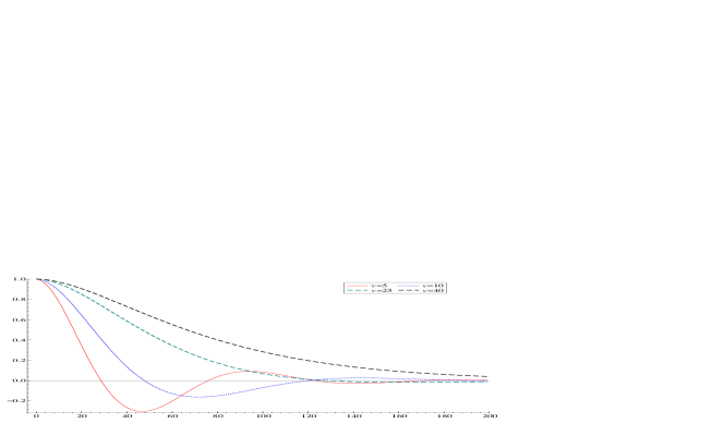
Figure 1: Plots of the determinants $\Lambda_{t}$ against $t$ for $\phi=0.975$, $\sigma_{\alpha}^{2}=0.5$ and four values of the approximating measurement variance $v$. Under Assumption (6), any negative values in the plot show that the second moment of the weights does not exist.

Figure 1 plots the determinants $\Lambda_{t}$ against $t$ when $n=2$, $\phi=0.975$, and $\sigma_{\alpha}^{2}=0.5$ for $v=5$, 10, 25 and 40. Since $v\geq\sigma_{\alpha}^{2}(1+|\phi|)/(1-|\phi|)=39.5$, $\Lambda_{t}$ decays exponentially only for $v=40$, with the three smaller values of $v$ resulting in complex roots in the difference equation (18), and therefore sinusoidal paths that cross the horizontal axis. If the model is less persistent, i.e. $\phi$ is smaller, then it is unnecessary for $v$ to be as large. For example, suppose that $n=2$, with $\sigma_{\alpha}^{2}=0.5$ as before and $\phi=0.6$. Then it is only necessary that $v\geq 2$ for the second moment to be finite.

Using the approximating state space model (20) with constant variance $v$ as the importance density may be inefficient because it does not depend on the $v_{t}$ which we estimate from the data. To take greater account of the computed $v_{t}$, let $v_{t}^{(0)}=v_{t}$, $C^{(0)}=\text{diag}(1/v_{1}^{(0)},...,1/v_{T}^{(0)})$, and $\epsilon>0$ be some small value. For $k=1,2,...$, define $v_{t}^{(k)}=v_{t}^{(k-1)}$ if $v_{t}^{(k-1)}\geq v$ and $v_{t}^{(k)}=v_{t}^{(k-1)}(1+\epsilon)$ if $v_{t}^{(k-1)}<v$. Let $C^{(k)}=\text{diag}(1/v_{1}^{(k)},...,1/v_{T}^{(k)})$. We suggest the following algorithm for finding the smallest $k\geq 0$ such that $Q-(n-1)C^{(k)}>0$.

Algorithm 1. Set $k=0$.

1. Check the positive definiteness of $Q-(n-1)C^{(k)}$ as in Section 4.2.1.

2. If it is positive definite then stop. Otherwise, set $k=k+1$ and go back to Step 1.

It is straightforward to see that the algorithm always converges, as with a large enough $k$, all the $v_{t}^{(k)}\geq v$ and therefore $Q-(n-1)C^{(k)}=Q-(n-1)C_{v}+(n-1)(C_{v}-C^{(k)})>0$. This justification does not mean that all $v_{t}^{(k)}\geq v$ after convergence. The motivation for Algorithm 1 is to adjust the data-based variances $v_{t}$ as little as possible while ensuring the existence of the required moments.

After the algorithm converges, let $C^{*}=C^{(k)}$ to obtain $Q-(n-1)C^{*}>0$. In practice, it is more efficient to use a mixture of two approximating Gaussian models in the form of (16), one with $\varepsilon_{t}\sim\textrm{\rm N}(0,v_{t}^{*})$ and the other with $\varepsilon_{t}\sim\textrm{\rm N}(0,v_{t})$, as justified by Proposition 3. We put a small weight $\pi=0.1$ on the former in all the examples below.

4.2.3 Checking and imposing the existence of moments for multivariate $\alpha_{t}$

Let $C^{(k)}=C^{(k-1)}/(1+\epsilon)$ for $k=1,2,...$ with $C^{(0)}=C$ and $\epsilon>0$ is a small number. The following algorithm provides a way to find the smallest $k$ such that $Q-(n-1)C^{(k)}>0$.

Algorithm 2. Set $k=0$.

1. Compute the smallest eigenvalue $\lambda_{\min}$ of $Q-(n-1)C^{(k)}$.

2. If $\lambda_{\min}>0$ then stop. Otherwise, set $k=k+1$ and go back to Step 1.

After convergence, as a by-product for checking the existence condition, a resulting $k>0$ means that the original $C$ fails the condition. Computing $\lambda_{\min}$ will be fast because $Q-(n-1)C^{(k)}$ is symmetric and block tridiagonal (Saad,, 2011). We now construct a mixture of two approximating Gaussian models (14) using the matrices $C$ and $C^{*}=C^{(k)}$.

4.3 Panel data models with an AR(1) latent process

The random effects models considered in Section 4.1 do not take into account time-varying individual effects. A possible way to overcome this is to include in the model a time-varying individual-specific effect $\alpha_{it}$. Let $y_{i}=(y_{i1},...,y_{iT_{i}})^{\prime}$, $i=1,...,m$, be panel data, which are modeled as

$$p(y_{it}|\beta,\alpha_{i})=\exp\left(\frac{y_{it}\eta_{it}-b(\eta_{it})}{\varpi}+c(y_{it},\varpi)\right),$$ (22)

with $\eta_{it}=x_{it}^{\prime}\beta+\alpha_{it},\ t=1,...,T_{i},\ i=1,...,m$, where the $x_{it}$ are $p$-vectors of covariates. The random effects $\alpha_{i}=(\alpha_{i1},...,\alpha_{iT_{i}})^{\prime}$ are assumed to follow the AR(1) process

$$\alpha_{i,t+1}=\mu(1-\phi)+\phi\alpha_{it}+\sigma u_{it},\;\;t=1,...,T_{i},$$

with $|\phi|<1$ and initial value $\alpha_{i1}\sim N(\mu,\sigma^{2}/(1-\phi^{2}))$, $u_{it}\stackrel{{\scriptstyle iid}}{{\sim}}N(0,1)$. The parameter vector $\psi$ consists of $\beta$, $\phi$ and $\sigma^{2}$. See, e.g., Bartolucci et al., (2012).

The likelihood is

$$L(\psi)=p(y|\psi)=\prod_{i=1}^{m}p(y_{i}|\psi)=\prod_{i=1}^{m}\int p(y_{i}|\alpha_{i},\psi)p(\alpha_{i}|\psi)d\alpha_{i},$$ (23)

which decomposes into a product of lower dimensional integrals, where

$$p(y_{i}|\alpha_{i},\psi)=\prod_{t=1}^{T_{i}}p(y_{it}|\beta,\alpha_{it})\,\;\;\text{and}\;\;p(\alpha_{i}|\psi)=p(\alpha_{i1})\prod_{t=1}^{T_{i}-1}p(\alpha_{i,t+1}|\alpha_{it}).$$

Each panel $y_{i}$ has the form of a non-Gaussian non-linear state space model (24) except that $T_{i}$ is often small, therefore the SPDK method can be used to obtain the importance parameters $\mu^{*}_{i}$ and ${Q^{*}_{i}}^{-1}$. Because the lengths $T_{i}$ of the panels are often small, we can use the general method in Section 3.1 to impose the condition for the existence of moments.

5 Illustrations

5.1 Illustrative example

Let $y=(y_{1},...,y_{N})$ be observations from a Bernoulli distribution with success probability $\alpha\in(0,1)$. The likelihood is

$$p(y|\alpha)=\prod_{i=1}^{N}\alpha^{y_{i}}(1-\alpha)^{1-y_{i}}=\alpha^{k}(1-\alpha)^{N-k},$$

with $k$ the total number of successes. We use a normal distribution $N(0.5,Q^{-1})$, with $Q=0.1$, truncated to the interval $(0,1)$ as a relatively uninformative prior on $\alpha$. That is, $p(\alpha)=C\kappa(\alpha)1_{(0,1)}(\alpha)$, where $\kappa(\alpha)=\exp\left(-\frac{1}{2}Q(\alpha-0.5)^{2}\right)$, with $C$ the normalizing constant such that $\int_{0}^{1}p(\alpha)d\alpha=1$. Suppose that we are interested in estimating the posterior mean of $\alpha$, i.e. we wish to estimate the integral $I=\int_{0}^{1}\alpha p(\alpha|y)d\alpha$ using importance sampling. Let $g(\alpha)$ be the importance density. Then the unnormalized weight is given by $w(\alpha)={1_{(0,1)}(\alpha)\kappa(\alpha)p(y|\alpha)}/{g(\alpha)}$. It is possible to use the Laplace method to construct a Gaussian importance density, but the constraint on the interval $(0,1)$ makes it difficult to find the mode of $p(\alpha|y)\propto p(\alpha)p(y|\alpha)$ when the mode is near either boundary. We instead use a second order Taylor expansion of $l(\alpha)=\log p(y|\alpha)$ at the MLE estimate $\widehat{\alpha}_{\text{mle}}=k/N$ of $\alpha$. Then, for all $\alpha\in(0,1)$,

$$\log p(y|\alpha)+\log p(\alpha) = \text{constant}+l(\alpha)-\frac{1}{2}Q(\alpha-0.5)^{2}$$

$$\simeq \text{constant}+l(\widehat{\alpha}_{\text{mle}})+\frac{1}{2}D(\alpha-\widehat{\alpha}_{\text{mle}})^{2}-\frac{1}{2}Q(\alpha-0.5)^{2}$$

$$= \text{constant}-\frac{1}{2}Q^{*}(\alpha-\alpha^{*})^{2},$$

where

$$D=\frac{\partial^{2}l(\alpha)}{\partial\alpha^{2}}\big{|}_{\alpha=\widehat{\alpha}_{\text{mle}}}=-\frac{k}{\widehat{\alpha}_{\text{mle}}^{2}}-\frac{N-k}{(1-\widehat{\alpha}_{\text{mle}})^{2}},\;\;Q^{*}=Q-D,\;\;\alpha^{*}=\frac{0.5Q-D\widehat{\alpha}_{\text{mle}}}{Q^{*}}.$$

Suppose that $g(\alpha)=N(\alpha|\alpha^{*},{Q^{*}}^{-1})$ is the importance density. Then the second moment of the unnormalized weight $E_{g}[w(\alpha)^{2}]$ is approximated as

$$E_{g}[w(\alpha)^{2}]\simeq K\int_{0}^{1}\exp\left(-\frac{1}{2}(2Q-Q^{*})(\alpha-\widetilde{\alpha})^{2}\right)d\alpha,$$

with $\widetilde{\alpha}=({Q-Q^{*}\alpha^{*}})/({2Q-Q^{*}})$ and a finite constant $K$. In theory, unlike the result in Proposition 1, this second moment exists even if $2Q-Q^{*}=Q+D<0$, because the integral is taken over the interval $(0,1)$ rather than the real line as in (2). However, in practice, this integral can be very large if $2Q-Q^{*}=Q+D\ll 0$. This is likely to happen as $D$ is often very small, especially in extreme cases where the underlying $\alpha$ is close to 0 or 1, while we need to keep $Q$ small enough in order to have a flat prior. We refer to this as the normal-IS case.

To demonstrate the theory presented in Section 3, we use a $2^{\text{nd}}$-moment constrained mixture importance sampler $g(\alpha)=\pi g_{1}(\alpha)+(1-\pi)g_{2}(\alpha)$ constructed as in Section 3.1. The heavy-tailed component $g_{1}(\alpha)$ with the weight $\pi=0.1$ is a normal density $N(\alpha^{*},{\widetilde{Q}}^{-1})$ with $\widetilde{Q}$ modified from $Q^{*}$ such that $2Q-\widetilde{Q}>0$, and $g_{2}(\alpha)$ is the original normal density $N(\alpha^{*},{Q^{*}}^{-1})$. We refer to this case as the $2^{\text{nd}}$-IS. Using a $t$ importance density rather than a normal importance density is sometimes recommended in the literature (Geweke,, 1989). As the third importance density, we use a $t$ density with location $\alpha^{*}$, scale ${Q^{*}}^{-1}$ and small degrees of freedom $\nu$. We set $\nu=5$ in this example after some experimentation and refer to this as the $t$-IS case.

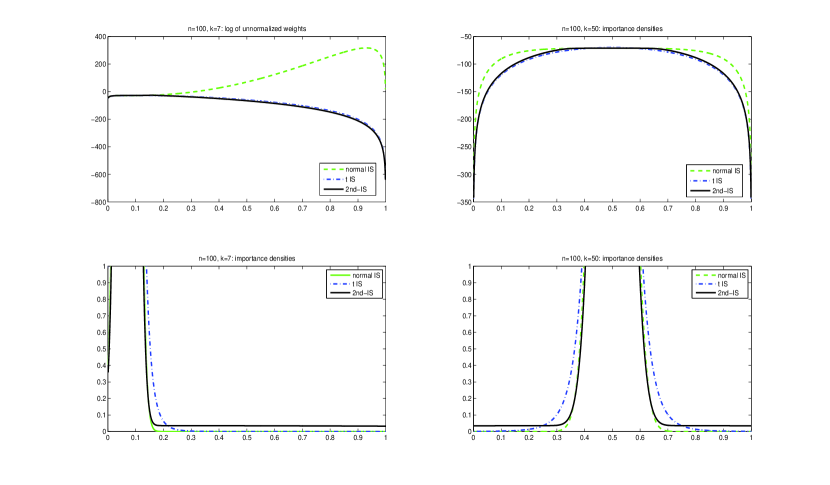
Figure 2: Bernoulli example: plots of the log weight functions $\log(w(\alpha))$ against $\alpha$ for three importance sampling approaches.

The first row of Figure 2 plots $\log(w(\alpha))$ against $\alpha$ for the three importance densities described above for two cases: a ‘hard’ case where $N=100$, $k=7$ and an ‘easy’ case where $N=100$, $k=50$. In the hard case the weight function $w(\alpha)$ of the normal-IS behaves badly for large $\alpha$, because the posterior is highly skewed to the right and the tail of the normal importance density declines much faster than the posterior. The figure shows that $t$-IS and $2^{\text{nd}}$-IS both avoid this problem. In the easy case, where the posterior is symmetric and is well approximated by a normal distribution, all the three weight functions appear well behaved. The panels in the second row plot the three importance densities, which show that imposing the condition leads to an importance density with the necessary heavy tails.

Let $\alpha_{s}\stackrel{{\scriptstyle iid}}{{\sim}}g(\alpha)$, $s=1,...,S=10^{6}$ be $S$ samples generated from the importance density $g(\alpha)$. The IS estimator of the integral $I$ and its asymptotic variance are (Geweke,, 1989)

$$\widehat{I}=\frac{\sum_{s=1}^{S}\alpha_{s}w(\alpha_{s})}{\sum_{s=1}^{S}w(\alpha_{s})},\;\;\;\;\widehat{\text{\rm Var}}(\widehat{I})=\frac{S\sum_{s=1}^{S}(\alpha_{s}-\widehat{I})^{2}w(\alpha_{s})^{2}}{\big{(}\sum_{s=1}^{S}w(\alpha_{s})\big{)}^{2}}.$$

We implemented the statistical test for finite variance by Koopman et al., (2009) (KSC). Define a sequence of $r$ random variables $Z_{1},\ldots,Z_{r}$ created from the importance weights that exceed a given threshold $u$ as $Z_{i}=\omega(\alpha_{i})-u$. The threshold $u$ is set to the $90^{\text{th}}$ percentile. Their test is based on the fact as $S$ and $u$ increase, the distribution of the excesses $Z_{1},\ldots,Z_{r}$ converges to the generalized Pareto distribution

$$f(z;\xi,\beta)=\frac{1}{\beta}\left(1+\xi\frac{z}{\beta}\right)^{-\frac{1}{\xi}-1}.$$

The shape parameter $\xi$ characterizes the thickness of the tails of the distribution. It can be shown that when $\xi>0$, $E_{g}[\omega(\alpha)^{n}]=\infty$ for $n\geq 1/\xi$. Hence, the variance of the importance weights is infinite when $\xi>1/2$. The Koopman et al., (2009) tests consists of obtaining a maximum likelihood estimate of $\xi$ and testing the null hypothesis that $\xi\leq 1/2$. We implement the Wald test version of their procedure and reject the hypothesis that the variance is finite if the returning $p$-value is smaller than 0.01.

Table 1 reports the following items averaged over 100 replications: (i) the estimate of the posterior mean $\widehat{I}$, (ii) the ratio of the asymptotic variance of $\widehat{I}$ for each IS approach divided by the asymptotic variance for the normal-IS, (iii) the proportion of the 100 replications in which the KSC test rejects the hypothesis of a finite variance, (iv) and the CPU time in seconds. In the “hard” case $N=100$ and $k=7$, the asymptotic variances of the $t$-IS and $2^{\text{nd}}$-IS are both small compared to that of the normal-IS, and the KSC test almost always rejects the hypothesis of a finite variance of the normal-IS. The improvement of the $2^{\text{nd}}$-IS over the normal-IS and $t$-IS is bigger when the ratio $k/N$ is closer to either 0 or 1. In the “easy” case $N=100$ and $k=50$, the normal IS has the smallest asymptotic variance, the KSC test indicates that all the variances are finite. However, we note that the loss in efficiency when using the $2^{\text{nd}}$-IS in the “easy” case is not as severe as the loss for the normal-IS in the “hard” case. That is, in general the $2^{\text{nd}}$-IS should be used if we do not have much information about the target density.

We found that the KSC test is very sensitive to the selection of the threshold $u$. In the examples follow we therefore do not compare our results to the test.

	$N=100,k=7$			$N=100,k=50$
Importance density	normal	$t$	$2^{\text{nd}}$-IS	normal	$t$	$2^{\text{nd}}$-IS
$\widehat{I}$	0.078	0.078	0.078	0.5	0.5	0.5
Variance ratio	1	0.38	0.34	1	1.83	1.20
KSC rejections	99	0	0	0	0	0
CPU time	0.24	0.39	0.35	0.26	0.39	0.37

Table 1: Bernoulli example: The table reports the estimate of the posterior mean, the ratio of the asymptotic variances, the KSC test rejections and the CPU times for the normal-IS, the $t$-IS and the $2^{\text{nd}}$-IS. All the values are averaged over 100 replications.

5.2 Likelihood evaluation for a non-Gaussian non-linear state space model

We consider a time series $\{y_{t},t=1,...,T\}$ generated from the dynamic Poisson model

$$p(y_{t}|\lambda_{t}) = \frac{\exp(-\lambda_{t})\lambda_{t}^{y_{t}}}{y_{t}!},\;\;\log(\lambda_{t})=\beta+\alpha_{t},$$ (24)

$$\alpha_{t+1} = \phi\alpha_{t}+\eta_{t},\;\;\eta_{t}\sim N(0,\sigma^{2}),\;\;\alpha_{1}\sim N(0,\sigma^{2}/(1-\phi^{2})).$$

We generate the data using the parameter values $\beta=-1.4$, $\phi=0.8$ and $\sigma^{2}=0.5(1-\phi^{2})$. The objective is to determine whether the importance weights from the SPDK importance sampling method for estimating the likelihood in model (24) have a finite variance. We also investigate the potential benefits of imposing a finite second moment using the $2^{\text{nd}}$-moment constrained mixture IS as in Section 4.2.

The simulation study generates 100 time series of length $T=500$ from model (24). Given the model parameter $\psi=(\beta,\phi,\sigma^{2})$, for each time series, we perform 100 likelihood evaluations at $\psi$ using $S=10^{4}$ importance samples for each likelihood evaluation. Table 2 reports the following performance measures averaged over the 100 realizations of the time series $\{y_{t},t=1,...,T\}$ and 100 evaluations: (i) the ratio of the variance of the weights; (ii) the ratio of the Monte Carlo standard errors (MCE) of the likelihood evaluations, with the SPDK sampler that does not impose the existence condition as the benchmark in both cases; (iii) the computing time per one likelihood evaluation; and (iv) the proportion of the 100 replications in which the original SPDK sampler satisfies the criterion (4) for the existence of the second moment.

	$\beta=-1.4,\phi=0.99,\sigma^{2}=1$		$\beta=-1.4,\phi=0.8,\sigma^{2}=0.18$
	not imposing	imposing	not imposing	imposing
Variance	1	0.0005	1	0.77
MCE	1	0.97	1	0.92
CPU (second)	0.46	0.52	0.21	0.23
Finite variance	0	-	0	-

Table 2: Likelihood evaluation for the Poisson state space model. The table reports the ratio of the variance of the weights, the ratio of the Monte Carlo standard errors (MCE) with the SPDK sampler without imposing the existence condition as the benchmark, the CPU time per likelihood evaluation, and the proportion of the 100 replications in which the original SPDK sampler satisfies the existence condition.

We estimate the likelihood for each simulated dataset at two different values of the model parameters $\psi$. The first parameter vector is $\psi=(-1.4,0.99,1)$, which represents an extreme case away from the DGP values. From Proposition 4, higher values of $\phi$ and $\sigma^{2}$ lead to a stricter restriction on the approximating linear state space model in order for the variance of the importance sampler to exist. In this case, imposing the existence condition leads to a substantial improvement in terms of both variance of the weights and the Monte Carlo errors of the likelihood evaluation. The original SPDK method always fails the criterion of Proposition 2 for the existence of the second moment. In the second case, we evaluate the likelihood at the true parameter values. In this case imposing the existence condition does not improve much on the original SPDK method. This result holds despite the theoretical infinite variance of the SPDK importance sampler.

5.3 Estimating a panel data model with autoregressive random effects

This simulation study estimates a panel data model with autoregressive random effects. We generate a data set from a Poisson longitudinal model

$$y_{it} \sim \text{Poisson}(\lambda_{it}),\;\;\lambda_{it}=\exp(x_{it}^{\prime}\beta+\alpha_{it}),$$

$$\alpha_{i,t+1} = \phi\alpha_{it}+\eta_{it},\;\;\alpha_{i1}\sim N(0,\sigma_{\alpha}^{2}),$$

$$\eta_{it} \stackrel{{\scriptstyle iid}}{{\sim}} N(0,\sigma^{2}),\;\;\sigma_{\alpha}^{2}=\sigma^{2}/(1-\phi^{2}),$$

with $t=1,...,T$ and $i=1,...,m$. We set $m=20$, $\beta=(1.4,-1)^{\prime}$, $\phi=0.8$, $x_{it}=(1,z_{it})^{\prime}$ with $z_{it}$ generated randomly from a uniform distribution on [0,1]. The unknown model parameters are $\psi=(\beta,\phi,\sigma^{2})$.

5.3.1 Likelihood estimation

We investigate the potential benefit of imposing the condition that the importance weights have a finite variance in the context of likelihood evaluation at a particular value of the model parameters. As noted in Section 4.3, the likelihood of this panel data model decomposes into a product of lower dimensional integrals. We estimate each of these integrals by first using the SPDK method to obtain the importance parameters, then construct the $2^{\text{nd}}$-moment constrained mixture IS as described in Section 3.1.

For the reasons discussed in Section 5.1, we compare this $2^{\text{nd}}$-IS to a $t$-IS with $\nu=5$ degrees of freedom, noting again that using such a $t$ importance density does not guarantee the existence of the second moments of the weights.

			Case 1			Case 2
$T$	$\sigma^{2}_{\alpha}$	Sampler	Variance	MCE	CPU	Variance	MCE	CPU
20	0.5	$t$-IS	1	1	0.15	1	1	0.17
		$2^{\text{nd}}$-IS	0.21	0.48	0.10	0.55	0.78	0.10
	1	$t$-IS	1	1	0.15	1	1	0.16
		$2^{\text{nd}}$-IS	0.32	0.59	0.10	0.57	0.79	0.10
50	0.5	$t$-IS	1	1	0.22	1	1	0.22
		$2^{\text{nd}}$-IS	0.23	0.50	0.18	0.48	0.76	0.16
	1	$t$-IS	1	1	0.22	1	1	0.22
		$2^{\text{nd}}$-IS	0.32	0.65	0.18	0.55	0.79	0.16

Table 3: Likelihood estimation for the panel data model. The table reports the ratio of the variance of weights and the ratio of the Monte Carlo standard errors (MCE) of the likelihood estimates with the $t$-IS as the benchmark. CPU is the computing time per one likelihood evaluation.

We draw 100 data sets from model (5.3) and perform 100 likelihood evaluations at a given model parameter vector $\psi$. We consider two different sets of the model parameters: in the first case $\psi$ is the vector of the true parameters that generate the data, and in the second case $\psi$ is set to $(0,0,0,1)$ which is far from the true values. We base each likelihood evaluation on $S=10^{3}$ importance samples. Common random numbers (CRN) are used. Similarly to Section 5.2, Table 3 reports the ratio of the variance of the weights, the ratio of the Monte Carlo standard errors (MCE) of the likelihood estimates with the $t$-IS as the benchmark, and computing time per one likelihood evaluation. Note that each likelihood evaluation consists of estimating $m$ separate integrals, so the variance reported here has been averaged over the $m$ panels. The simulation results suggest that it is beneficial to impose the condition that the importance weights have a finite variance.

Table 3 also shows that although imposing the existence of the second moments takes extra CPU time, the $2^{\text{nd}}$-IS method overall takes less time than the $t$-IS because working with a $t$ distribution takes more time than working with the constrained Gaussian mixture density.

5.3.2 Bayesian inference

This section explores the potential benefit of imposing the existence condition in the context of Bayesian inference. Bayesian inference for the panel data model (5.3) can be carried out using the MCMC approach to sample from the posterior $p(\psi|y)$, in which the likelihood used within the Metropolis-Hastings algorithm is estimated unbiasedly by importance sampling. We put a normal prior $N(0,\tau_{0}I_{p})$ on $\beta$, a reference prior $p(\phi)\propto 1/\sqrt{1-\phi^{2}}$ on the correlation coefficient $\phi$ (Berger and Yang,, 1994) and $p(\sigma^{2})\propto 1/\sigma^{2}$, and set $\tau_{0}=100$.

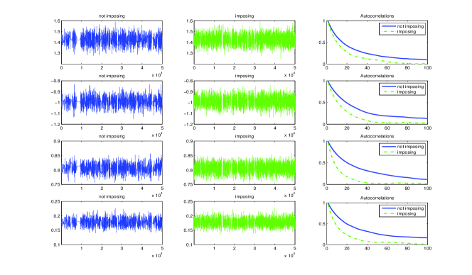
Figure 3: Panel data model example. Plots of the MCMC chains and autocorrelations for $\beta$, $\phi$ and $\sigma^{2}$ for the case with $T=80$ and $\sigma^{2}_{\alpha}=1$.

We consider two MCMC samplers. The first sampler uses the $2^{\text{nd}}$-IS to estimate the likelihood to ensure the finite second moment of the importance weights, and leads to a finite variance of the log likelihood estimator which is important for MCMC simulation based on an estimated likelihood (Pitt et al.,, 2012). The second MCMC sampler uses the $t$-IS as in Section 5.3.1 to estimate the likelihood. Each sampler is run for 50,000 iterations after 50,000 burn-in iterations using $S=200$ importance samples to estimate each likelihood. The Markov chains are drawn by the adaptive random walk Metropolis-Hastings algorithm in Haario et al., (2001).

We use the integrated autocorrelation time (IACT) and the acceptance rate of the Metropolis-Hastings algorithm as the performance measures. For a scalar parameter $\theta$ the IACT is defined as (Liu,, 2001)

$$\text{IACT}=1+2\sum_{j=1}^{\infty}\rho_{j},$$

where $\rho_{j}$ is the $j$th lag autocorrelation of the iterates of $\theta$ in the MCMC scheme. We estimate the IACT by

$$\widehat{\text{IACT}}=1+2\sum_{j=1}^{L^{*}}\widehat{\rho}_{j},$$

where $\widehat{\rho}_{j}$ is the $j$th lag sample autocorrelation and $L^{*}=\min\{1000,L\}$, with $L$ the first index $j$ such that $|\widehat{\rho}_{j}|\leq 2/\sqrt{K}$ where $K$ is the sample size used to estimate $\widehat{\rho}_{j}$. When summarizing the performance of the MCMC with $d$ parameters estimated, we report, for simplicity, the average IACT over the $d$ parameters.

We investigate the performance of the two MCMC samplers for four combinations of $T$ and $\sigma^{2}$. Figures 3 plot the iterates and the autocorrelations for the four parameters $\beta$ (first two rows), $\phi$ (third) and $\sigma^{2}$ (last) for the case with $\sigma^{2}_{\alpha}=1$ and $T=80$, which shows that the sampler which imposes the existence condition works better. Table 4 summarizes the acceptance rates and the IACT ratios averaged over 5 replications. The table also reports the CPU time taken for each MCMC iteration. The results suggest that the new method is beneficial in cases with large $\sigma^{2}$, after taking into account the higher computing time required to impose the variance existence condition.

$T$	$\sigma^{2}_{\alpha}$	Imposing	Acc. rate (%)	IACT ratio	CPU (second)
20	0.5	No	20	1	0.015
		Yes	25	0.79	0.033
	1	No	6	1	0.016
		Yes	12	0.34	0.033
80	0.5	No	20	1	0.064
		Yes	23	0.95	0.135
	1	No	1.8	1	0.061
		Yes	4.8	0.54	0.132

Table 4: Bayesian inference for the panel data model. The table reports the acceptance rates (Acc. rate), the integrated autocorrelation time (IACT) ratios with the MCMC sampler that does not impose the existence condition as the benchmark, and the CPU time taken for each MCMC iteration. All values are averaged over 5 replications.

5.4 An application to the anti-epileptic drug dataset

The anti-epileptic drug longitudinal dataset (see, e.g., Fitzmaurice et al.,, 2011, p.346) consists of seizures counts on 59 epileptic patients over 5 time-intervals of treatment. The objective is to study the effects of the anti-epileptic drug on the patients. Following Fitzmaurice et al., (2011), we consider the mixed effects Poisson regression model

$$p(y_{ij}|\beta,\alpha_{i}) = \text{Poisson}(\exp(\eta_{ij})),$$

$$\eta_{ij} = c_{ij}+\beta_{1}+\beta_{2}\text{time}_{ij}+\beta_{3}\text{treatment}_{ij}+\beta_{4}\text{time}_{ij}\times\text{treatment}_{ij}$$

$$+\alpha_{i1}+\alpha_{i2}\text{time}_{ij},$$

$j=0,1,...,4$, $i=1,...,59$ and $c_{ij}$ is an offset. As in Fitzmaurice et al., (2011), the offset $c_{ij}=\log(8)$ if $j=0$ and $c_{ij}=\log(2)$ for $j>0$, $\text{time}_{ij}=j$, $\text{treatment}_{ij}=0$ if patient $i$ is in the placebo group and $\text{treatment}_{ij}=1$ if in the treatment group. The $\alpha_{i}=(\alpha_{i1},\alpha_{i2})^{\prime}\sim N(0,Q^{-1})$ are random effects that need to be integrated out. We consider a normal prior $N_{p}(0,\tau_{0}I_{p})$ for $\beta$ and a Wishart $\mathcal{W}(\nu_{0},\tau_{0}I_{u})$ prior for the precision $Q$. In order to have flat priors, we select $\tau_{0}=1000$, $\nu_{0}=u+1$. In the MCMC scheme, we first use the Leonard and Hsu transformation $Q=\exp(\Sigma)$, where $\Sigma$ is an unconstrained symmetric matrix, and reparameterize $Q$ by the lower-triangle elements $\theta_{Q}$ of $\Sigma$, which is an one-to-one transformation between $Q$ and $\theta_{Q}$. We then use the adaptive random walk Metropolis-Hastings algorithm in Haario et al., (2001) to sample from the posterior $p(\beta,\theta_{Q}|y)$. The dimension of $\psi=(\beta,\theta_{Q})$ is $4+2(2+1)/2=7$.

Similarly to Section 5.3.2, we run two MCMC samplers based on $2^{\text{nd}}$-IS and $t$-IS. Each sampler is run for 50000 iterations after discarding 50000 burn-in iterations. The number of samples used in each likelihood estimation is $S=200$. Figure 4 plots the iterates of the parameters as well as the autocorrelations generated by the two samplers. The IACT values of the samplers imposing and not imposing the existence condition are 19.6 and 29.2. That is, imposing the condition leads to a sampler that is roughly 1.5 times more efficient than not imposing. The acceptance rates averaged over replications of the sampler imposing and not imposing the existence condition are 22.3% and 18.8%, respectively. This suggests that it is beneficial to impose the finite second moment condition of the importance weight within a MCMC sampler. The two samplers respectively take 0.079 and 0.058 seconds to run each MCMC iteration.

Figure 4: Drug example: The figure plots the marginal chains and their corresponding first 100 autocorrelations, generated by the MCMC sampler based on the $2^{\text{nd}}$-IS (green) and the MCMC sampler based on the $t$-IS (blue).

Appendix A

Proof of Proposition 1.

Let $\text{const}_{1}$, $\text{const}_{2}$,… be generic constants. By equation (3)

$$\log\omega(\alpha) =l(\alpha)+\log p(\alpha)-\log g(\alpha)$$

$$\leq\text{const}_{1}-\frac{1}{2}(\alpha-\xi)^{\prime}Q(\alpha-\xi)+\frac{1}{2}(\alpha-\mu^{\ast})^{\prime}Q^{\ast}(\alpha-\mu^{\ast})$$

$$=\text{const}_{2}+\frac{1}{2}(\alpha-\mu^{+})^{\prime}Q^{+}(\alpha-\mu^{+}),$$

where $Q^{+}=Q^{\ast}-Q$, $\mu^{+}=\left(Q^{+}\right)^{-1}(Q^{\ast}\mu^{\ast}-Q\xi)$. Hence

$$n\log\omega(\alpha)\leq\text{const}_{3}+\frac{1}{2}(\alpha-\mu^{+})^{\prime}nQ^{+}(\alpha-\mu^{+}),$$

and

$$E_{g}[\omega(\alpha)^{n}] \leq\text{const}_{4}\times\int\exp\left\{\frac{1}{2}(\alpha-\mu^{+})^{\prime}nQ^{+}(\alpha-\mu^{+})\right\}g(\alpha)d\alpha$$

$$=\text{const}_{5}\times\int\exp\left\{-\frac{1}{2}(\alpha-a^{+})^{\prime}V(\alpha-a^{+})\right\}d\alpha,$$

where $V=Q^{\ast}-nQ^{+}=Q^{\ast}-n(Q^{\ast}-Q)$, $Va^{+}=Q^{\ast}\mu^{\ast}-nQ^{+}\mu^{+}$. Since $V=Q^{\ast}-n(Q^{\ast}-Q)>0$ by assumption, the integrand in the last equation corresponds to the kernel of a multivariate Gaussian density. The integral is therefore finite. ∎

Proof of Proposition 2.

Proof of (i) follows directly from Proposition 1. To prove (ii), let $V=Q^{\ast}-n(Q^{\ast}-Q)<0$.

$$\log\omega(\alpha) =l(\alpha)+\log p(\alpha)-\log g(\alpha)$$

$$=\text{const}_{1}+l(\alpha)-\frac{1}{2}(\alpha-\xi)^{\prime}Q(\alpha-\xi)+\frac{1}{2}(\alpha-\mu^{\ast})^{\prime}Q^{\ast}(\alpha-\mu^{\ast})$$

$$=\text{const}_{2}+l(\alpha)+\frac{1}{2}(\alpha-\mu^{+})^{\prime}Q^{+}(\alpha-\mu^{+}),$$

where $Q^{+}=Q^{*}-Q$. So

$$E_{g}[\omega(\alpha)^{n}] =\text{const}_{3}\times\int_{\mathbb{R}^{d}}\exp\left\{nl(\alpha)+\frac{1}{2}(\alpha-\mu^{+})^{\prime}nQ^{+}(\alpha-\mu^{+})\right\}g(\alpha)d\alpha$$

$$=\text{const}_{4}\times\int_{\mathbb{R}^{d}}\exp\left\{nl(\alpha)+\zeta^{\prime}\alpha-\frac{1}{2}\alpha^{\prime}V\alpha\right\}d\alpha,$$

where $\zeta$ is a constant vector. We can write $\frac{1}{2}\alpha^{\prime}V\alpha=\frac{1}{2}v_{jj}\alpha_{j}^{2}+B\alpha_{j}+C$, where $v_{jj}<0$ as $V<0$ and $B$ and $C$ involve only $\alpha_{-j}=(\alpha_{1},...,\alpha_{j-1},\alpha_{j+1},...,\alpha_{d})^{\prime}$. The moment $E_{g}[\omega(\alpha)^{n}]$ can now be written as

$$E_{g}[\omega(\alpha)^{n}] =\text{const}_{4}\times\int_{\mathbb{R}^{d-1}}\left(\int_{\mathbb{R}}\exp\left\{nl(\alpha)+\zeta^{\prime}\alpha-\frac{1}{2}v_{jj}\alpha_{j}^{2}-B\alpha_{j}-C\right\}d\alpha_{j}\right)d\alpha_{-j}.$$

By (6), for any fixed $\alpha_{-j}$,

$$nl(\alpha)+d^{\prime}\alpha-\frac{1}{2}v_{jj}\alpha_{j}^{2}-B\alpha_{j}-C=\alpha_{j}^{2}\left(-\frac{1}{2}v_{jj}+\frac{nl(\alpha)+d^{\prime}\alpha-B\alpha_{j}-C}{\alpha_{j}^{2}}\right)\longrightarrow+\infty$$

when either $\alpha_{j}\to-\infty$ or $\alpha_{j}\to+\infty$. It follows that the integral over $\alpha_{j}$ is infinite for any fixed $\alpha_{-j}$, thus $E_{g}[\omega(\alpha)^{n}]$ is infinite. ∎

Proof of Proposition 3.

Since $g(\alpha)\geq\pi g_{1}(\alpha)$, $\sup(g)\supseteq\sup(g_{1})\supseteq\sup(f)$.

$$\int_{\sup(g)}\left(\frac{f(\alpha)}{g(\alpha)}\right)^{n}g(\alpha)d\alpha = \int_{\sup(g_{1})}\left(\frac{f(\alpha)}{g(\alpha)}\right)^{n}g(\alpha)d\alpha+\int_{\sup(g)\setminus\sup(g_{1})}\left(\frac{f(\alpha)}{g(\alpha)}\right)^{n}g(\alpha)d\alpha$$

$$= A+B.$$

We have

$$A=\int_{\sup(g_{1})}\left(\frac{f(\alpha)}{g(\alpha)}\right)^{n}g(\alpha)d = \int_{\sup(g_{1})}\left(\frac{f(\alpha)}{g_{1}(\alpha)}\right)^{n}\left(\frac{g_{1}(\alpha)}{g(\alpha)}\right)^{n-1}g_{1}(\alpha)d\alpha$$

$$\leq \frac{1}{\pi^{n-1}}\int_{\sup(g_{1})}\left(\frac{f(\alpha)}{g_{1}(\alpha)}\right)^{n}g_{1}(\alpha)d\alpha<\infty.$$

If $\sup(g)\setminus\sup(g_{1})=\emptyset$, $B=0$. Otherwise, $f(\alpha)=0$ on $\sup(g)\setminus\sup(g_{1})$, and therefore $B=0$. This completes the proof. ∎

Proof of Proposition 4.

From Proposition 2, we need to have $Q-(n-1)C>0$. This is equivalent to having all the determinants $\Lambda_{t}>0$, $t=1,...,T-1$ and $\widetilde{\Lambda}_{T}>0$, where the $\Lambda_{t}$ and $\widetilde{\Lambda}_{T}$ are given in (18) and (19), with $v_{t}=v$. Let $c=1+\phi^{2}-\sigma^{2}(n-1)/v$. The general solution of the recursion equation (18) is a linear combination of the powers of the roots of the characteristic polynomial

$$r^{2}-cr+\phi^{2}=0$$ (25)

if the roots are unequal, as we discuss bellow.

Consider first the case where $v>(n-1)\sigma^{2}_{\alpha}(1+|\phi|)/(1-|\phi|)=(n-1)\sigma^{2}/(1-|\phi|)^{2}$. Then $c>2|\phi|$, which ensures that the characteristic polynomial (25) has two distinct and positive roots $r_{1}={c}/{2}+\frac{1}{2}\sqrt{c^{2}-4\phi^{2}}$ and $r_{2}={c}/{2}-\frac{1}{2}\sqrt{c^{2}-4\phi^{2}}$. Hence the general solution to the second-order difference equation (18) is

$$\Lambda_{t}=Kr_{1}^{t}+Lr_{2}^{t},\;\;t=0,...,T-1,$$

where $K,L$ are constants determined by the boundary conditions $K+L=1$ and $Kr_{1}+Lr_{2}=\Lambda_{1}$. Note that $v>(n-1)\sigma^{2}/(1-|\phi|)^{2}>(n-1)\sigma^{2}$, which implies that $\Lambda_{1}=1-(n-1)\sigma^{2}/v>0$. Using the boundary conditions, we obtain

$$K=\frac{c-\phi^{2}-r_{2}}{r_{1}-r_{2}},\;\;L=\frac{r_{1}-c+\phi^{2}}{r_{1}-r_{2}}.$$

As $r_{2}<c/2$, $|\phi|<1$ and $r_{1}>r_{2}$, we have that $K>(c/2-\phi^{2})/(r_{1}-r_{2})>(|\phi|-\phi^{2})/(r_{1}-r_{2})>0$. Therefore, for $t=0,...,T-1$,

$$\Lambda_{t}=Kr_{1}^{t}+(1-K)r_{2}^{t}=K(r_{1}^{t}-r_{2}^{t})+r_{2}^{t}>0.$$

We now check that $\widetilde{\Lambda}_{T}>0$ as well, by observing that for any $t\geq 0$,

$$\Lambda_{t}=Kr_{1}^{t}+Lr_{2}^{t} =\frac{c-\phi^{2}-r_{2}}{r_{1}-r_{2}}r_{1}^{t}+\frac{r_{1}-c+\phi^{2}}{r_{1}-r_{2}}r_{2}^{t}$$

$$=\frac{cr_{1}^{t}-\phi^{2}r_{1}^{t}-\phi^{2}r_{1}^{t-1}}{r_{1}-r_{2}}+\frac{\phi^{2}r_{2}^{t-1}-cr_{2}^{t}+\phi^{2}r_{2}^{t}}{r_{1}-r_{2}}$$

$$=\frac{r_{1}^{t-1}(cr_{1}-\phi^{2})-\phi^{2}r_{1}^{t}}{r_{1}-r_{2}}+\frac{r_{2}^{t-1}(\phi^{2}-cr_{2})+\phi^{2}r_{2}^{t}}{r_{1}-r_{2}}$$

$$=\frac{r_{1}^{t+1}-\phi^{2}r_{1}^{t}}{r_{1}-r_{2}}+\frac{-r_{2}^{t+1}+\phi^{2}r_{2}^{t}}{r_{1}-r_{2}}$$

$$=\frac{r_{1}^{t+1}-r_{2}^{t+1}-\phi^{2}(r_{1}^{t}-r_{2}^{t})}{r_{1}-r_{2}}.$$

In the above, we use the fact that $r_{1}r_{2}=\phi^{2}$ and $cr_{i}-\phi^{2}=r_{i}^{2}$, $i=1,2$. Hence,

$$\widetilde{\Lambda}_{T} =\left(\{1+\phi^{2}-(n-1)\sigma^{2}/v\}\Lambda_{T-1}-\phi^{2}\Lambda_{T-2}\right)-\phi^{2}\Lambda_{T-1}$$

$$=\Lambda_{T}-\phi^{2}\Lambda_{T-1}$$

$$=\frac{r_{1}^{T+1}-r_{2}^{T+1}-\phi^{2}(r_{1}^{T}-r_{2}^{T})}{r_{1}-r_{2}}-\phi^{2}\frac{r_{1}^{T}-r_{2}^{T}-\phi^{2}(r_{1}^{T-1}-r_{2}^{T-1})}{r_{1}-r_{2}}$$

$$=\frac{r_{1}^{T-1}(r_{1}-\phi^{2})^{2}-r_{2}^{T-1}(r_{2}-\phi^{2})^{2}}{r_{1}-r_{2}}.$$

It is easy to check that $-(r_{1}-\phi^{2})<r_{2}-\phi^{2}<r_{1}-\phi^{2}$, thus $(r_{2}-\phi^{2})^{2}<(r_{1}-\phi^{2})^{2}$. This, together with $r_{1}>r_{2}$, implies that $\widetilde{\Lambda}_{T}>0$.

Consider the case where $v=(n-1)\sigma^{2}_{\alpha}(1+|\phi|)/(1-|\phi|)=(n-1)\sigma^{2}/(1-|\phi|)^{2}$. The characteristic polynomial (25) has two equal roots $r_{1}=r_{2}=r=|\phi|$. Then the solution to the difference equation (18) is $\Lambda_{t}=(A_{0}+A_{1}t)r^{t}$ with $A_{0}=1$ and $A_{1}=1-|\phi|$. If $\phi\not=0$, it is obvious that $\Lambda_{t}>0$ for $t=0,...,T-1$, and for $t=T$,

$$\widetilde{\Lambda}_{T}=\Lambda_{T}-\phi^{2}\Lambda_{T-1} =(A_{0}+A_{1}T)r^{T}-\phi^{2}\big{(}(A_{0}+A_{1}(T-1))r^{T-1}\big{)}$$

$$=|\phi|^{T}(1-|\phi|)(1+|\phi|+T(1-|\phi|))>0.$$

This completes the proof. ∎

Appendix B

Shephard and Pitt, (1997) and Durbin and Koopman, (1997) construct an importance sampler based on the following approximation of the target density

$$\log p(y|\alpha)+\log p(\alpha) =l(\alpha)-\frac{1}{2}(\alpha-\mu)^{T}Q(\alpha-\mu)$$

$$\simeq l(\widehat{\alpha})+(\alpha-\widehat{\alpha})^{T}l^{\prime}(\widehat{\alpha})-\frac{1}{2}(\alpha-\widehat{\alpha})^{T}C(\alpha-\widehat{\alpha})-\frac{1}{2}(\alpha-\mu)^{T}Q(\alpha-\mu),$$

where $\widehat{\alpha}$ is the mode of $p(y|\alpha)p(\alpha)$ and $C$ is minus the Hessian of $l(\alpha)$ at $\widehat{\alpha}$. In the framework of equation (13), $B=l^{\prime}(\widehat{\alpha})+C\widehat{\alpha}$.

We can find the mode of $p(y|\alpha)p(\alpha)$ by using the following iterative algorithm, which is equivalent to a Newton-Raphson procedure for finding the maximum of the target density as a function of $\alpha$.

Algorithm: Constructing the SPDK importance density

1. Start with an initial guess $\widehat{\alpha}$.

2. While convergence criterion is not met do

   • Calculate the matrix of second derivatives $C\leftarrow-\left.\frac{\partial^{2}l(\alpha)}{\partial\alpha\partial\alpha^{\prime}}\right|_{\alpha=\widehat{\alpha}}$

   • Update the other importance parameter $B\leftarrow l^{\prime}(\widehat{\alpha})+C\widehat{\alpha}$.

   • Update the covariance matrix $Q^{\ast-1}\leftarrow(C+Q)^{-1}$.

   • Update the estimate of the mode $\widehat{\alpha}\leftarrow Q^{\ast-1}(B+Q\mu)$.

3. Set the mean of the importance density as $\mu^{\ast}=\widehat{\alpha}$.

Shephard and Pitt, (1997) and Durbin and Koopman, (1997) show how to carry out the above computations efficiently using the Kalman filter and smoother for the state space model of Section 4.2. In this case, it is unnecessary to calculate the items in Algorithm 1 explicitly, except for the mode. For this class of models, we can also obtain near optimal importance parameters $\left\{b_{t},C_{t}\right\}$ for $t=1,\ldots,T$ by using the NAIS method of Koopman et al., (2012). The method is based on recursively minimising

$$\underset{\chi_{t}}{\min}\int\lambda^{2}(\alpha_{t},y_{t};\psi)g(\alpha_{t}|y;\psi)\,\textrm{d}\alpha_{t}$$ (26)

where

$$\lambda(\alpha_{t},y_{t};\psi)=\log p(y_{t}|\alpha_{t};\psi)-a_{t}-b_{t}^{\prime}\,\alpha_{t}+\frac{1}{2}\alpha_{t}^{\prime}C_{t}\alpha_{t},$$ (27)

for $t=1,\ldots,T$, given the current estimates of the optimal importance parameters. We obtain $g(\alpha_{t}|y;\psi)$ by the Kalman filter and smoother and evaluate the integral (26) by numerical integration (in the univariate state case). Due to the linearity of $\lambda(\theta_{t},y_{t};\psi)$, the minimisation consists of a weighted OLS regression.

Appendix C

We make $\widetilde{\lambda}_{j}$ continuous in $\lambda_{j}$ by defining

$$\widetilde{\lambda}_{j}=\begin{cases}\lambda_{j},&\text{if}\;\;\lambda_{j}<\frac{1-\epsilon}{n-1},\\ \frac{1-\epsilon}{n-1},&\text{if}\;\;\lambda_{j}\geq\frac{1-\epsilon}{n-1}.\end{cases}$$ (28)

Then we still have that $nQ-(n-1)\widetilde{Q}=AV(I-(n-1)\widetilde{\Lambda})V^{\prime}A^{\prime}>0$ because $\widetilde{\lambda}_{j}<1/(n-1)$ for all $j$. However, the $\widetilde{\lambda}_{j}$ in (28) is not a differentiable function of $\lambda_{j}$. To make $\widetilde{Q}$ continuous and differentiable in $\psi$, we proceed as follows. Let $\delta>0$ be some small number and denote $\tau=(1-\epsilon)/(n-1)$. We define

$$\widetilde{\lambda}_{j}=\begin{cases}\lambda_{j},&\text{if}\;\;\lambda_{j}<\tau-\delta,\\ f(\lambda_{j}),&\text{if}\;\;\tau-\delta\leq\lambda_{j}<\tau,\\ \tau,&\text{if}\;\;\lambda_{j}\geq\tau,\end{cases}$$ (29)

where $f(\lambda_{j})=a\lambda_{j}^{3}+b\lambda_{j}^{2}+c\lambda_{j}+d$ satisfying $f(\tau-\delta)=\tau-\delta$, $f(\tau)=\tau$, $\dot{f}(\tau-\delta)=1$ and $\ddot{f}(\tau)=0$. Then $\widetilde{\lambda}_{j}$ defined in (29) is continuous and differentiable in $\lambda_{j}$. After some algebra, we obtain $a=-1/\delta^{2}$, $b=3\tau/\delta^{2}-2/\delta$, $c=4\tau/\delta-3\tau^{2}/\delta^{2}$ and $d=\tau+\tau^{3}/\delta^{2}-2\tau^{2}/\delta$. Now, $h(\lambda_{j})=f^{\prime}(\lambda_{j})=3a\lambda_{j}^{2}+2b\lambda_{j}+c$ is an open-down parabola with $h(\tau-\delta)=1$ and $h(\tau)=0$, which implies that $h(\lambda_{j})\geq 0$ for all $\lambda_{j}$ in the interval $(\tau-\delta,\tau)$. It follows that $f(\lambda_{j})\leq f(\tau)=\tau$ for all $\lambda_{j}\in(\tau-\delta,\tau)$. We have proved that $\widetilde{\lambda}_{j}\leq\tau<1/(n-1)$, which ensures that $nQ-(n-1)\widetilde{Q}=AV(I-(n-1)\widetilde{\Lambda})V^{\prime}A^{\prime}>0$ as required. In our implementation we take $\delta=\epsilon=10^{-5}$.

Appendix D

Recall that the latent $\alpha_{t}$ follows an AR(1) process $\alpha_{t+1}=d+\Phi\alpha_{t}+\eta_{t}$, $t=1,...,T-1$ with $\alpha_{1}\sim N(\mu,\Sigma_{\alpha})$ and $\eta_{t}\sim N(0,\Sigma)$. For any $\tau\geq 1$, let

$$\Gamma(\tau) =\text{cov}(\alpha_{t+1},\alpha_{t+1-\tau})=\Phi\text{cov}(\alpha_{t},\alpha_{t+1-\tau})=\Phi\Gamma(\tau-1).$$

For $\tau=0$, $\Sigma_{\alpha}=\Gamma(0)$ satisfies the following equation

$$\Sigma_{\alpha}=\text{cov}(\alpha_{t+1},\alpha_{t+1})=\Phi\text{cov}(\alpha_{t},\alpha_{t})\Phi^{\prime}+\Sigma=\Phi\Sigma_{\alpha}\Phi^{\prime}+\Sigma.$$ (30)

The covariance matrix of $\alpha=(\alpha_{1}^{\prime},...,\alpha_{T}^{\prime})^{\prime}$ is

$$Q^{-1}=\begin{pmatrix}\Sigma_{\alpha}&(\Phi\Sigma_{\alpha})^{\prime}&...&(\Phi^{T-1}\Sigma_{\alpha})^{\prime}\\ \Phi\Sigma_{\alpha}&\Sigma_{\alpha}&...&(\Phi^{T-2}\Sigma_{\alpha})^{\prime}\\ \vdots&\vdots&\ddots&\vdots\\ \Phi^{T-1}\Sigma_{\alpha}&\Phi^{T-2}\Sigma_{\alpha}&...&\Sigma_{\alpha}\end{pmatrix}.$$

It can be shown that the inverse of this matrix is

$$Q=\begin{pmatrix}\Sigma_{\alpha}^{-1}(I+\Phi(I-\Phi^{2})^{-1}\Phi)&-\widetilde{\Phi}&0&...&0&0\\ -\widetilde{\Phi}&\widetilde{\Gamma}&-\widetilde{\Phi}&...&0&0\\ \vdots&\vdots&\vdots&&\vdots&\vdots\\ 0&0&0&...&\widetilde{\Gamma}&-\widetilde{\Phi}\\ 0&0&0&...&-\widetilde{\Phi}&\Sigma_{\alpha}^{-1}(I-\Phi^{2})^{-1}\end{pmatrix},$$

where $\widetilde{\Phi}=\Sigma_{\alpha}^{-1}\Phi(I-\Phi^{2})^{-1}$ and $\widetilde{\Gamma}=\Sigma_{\alpha}^{-1}(I-\Phi^{2})^{-1}+\Sigma_{\alpha}^{-1}\Phi(I-\Phi^{2})^{-1}\Phi$.

If $\alpha_{t}$ is scalar as in model (15), then using the notation in Section 4.2.1, $\Phi,\Sigma_{\alpha},\Sigma$ become $\phi,\sigma_{\alpha}^{2},\sigma^{2}$ respectively. Solving $\Sigma_{\alpha}$ in (30) gives $\sigma_{\alpha}^{2}=\sigma^{2}/(1-\phi^{2})$ and

$$Q=\begin{pmatrix}1/\sigma^{2}&-\phi/\sigma^{2}&0&...&0&0\\ -\phi/\sigma^{2}&(1+\phi^{2})/\sigma^{2}&-\phi/\sigma^{2}&...&0&0\\ \vdots&\vdots&\vdots&&\vdots&\vdots\\ 0&0&0&...&(1+\phi^{2})/\sigma^{2}&-\phi/\sigma^{2}\\ 0&0&0&...&-\phi/\sigma^{2}&1/\sigma^{2}\end{pmatrix}.$$

References

- Andrieu and Roberts, (2009) Andrieu, C. and Roberts, G. (2009). The pseudo-marginal approach for efficient Monte Carlo computations. The Annals of Statistics, 37:697–725.
- Bartolucci et al., (2012) Bartolucci, F., Farcomeni, A., and Pennoni, F. (2012). Latent Markov Models for Longitudinal Data. Chapman and Hall/CRC press.
- Bauwens and Galli, (2009) Bauwens, L. and Galli, F. (2009). Efficient importance sampling for ML estimation of SCD models. Computational Statistics and Data Analysis, 53(6):1974–1992.
- Bauwens and Hautsch, (2006) Bauwens, L. and Hautsch, N. (2006). Stochastic conditional intensity processes. Journal of Financial Econometrics, 4(3):450–493.
- Bazaraa et al., (2006) Bazaraa, M. S., Sherali, H. D., and Shetty, C. M. (2006). Nonlinear Programming. Wiley, New Jersey, 3rd edition.
- Berger and Yang, (1994) Berger, J. O. and Yang, R.-Y. (1994). Noninformative priors and Bayesian testing for the AR(1) model. Econometric Theory, 10(3-4):461–482.
- Berry, (1941) Berry, A. C. (1941). The accuracy of the Gaussian approximation to the sum of independent variates. Transactions of the American Mathematical Society, 49:122–136.
- Chen and Shao, (2004) Chen, L. H. Y. and Shao, Q.-M. (2004). Normal approximation under local dependence. The Annals of Probability, 32(3A):1985–2028.
- de Jong and Shephard, (1995) de Jong, P. and Shephard, N. (1995). The simulation smoother for time series models. Biometrika, 82:339–350.
- Durbin and Koopman, (1997) Durbin, J. and Koopman, S. J. (1997). Monte Carlo maximum likelihood estimation for non-Gaussian state space models. Biometrika, (84):669–684.
- Durbin and Koopman, (2000) Durbin, J. and Koopman, S. J. (2000). Time series analysis of non-Gaussian observations based on state space models from both classical and Bayesian perspectives. Journal of the Royal Statistical Society, Series B, (62):3–56.
- Durbin and Koopman, (2001) Durbin, J. and Koopman, S. J. (2001). Time Series Analysis by State Space Methods. Oxford University Press.
- Durbin and Koopman, (2002) Durbin, J. and Koopman, S. J. (2002). A simple and efficient simulation smoother for state space time series analysis. Biometrika, (89):603–616.
- Esseen, (1942) Esseen, C.-G. (1942). On the Liapunoff limit of error in the theory of probability. Arkiv for matematik, astronomi och fysik, A28:1–19.
- Fitzmaurice et al., (2011) Fitzmaurice, G. M., Laird, N. M., and Ware, J. H. (2011). Applied Longitudinal Analysis. John Wiley & Sons, Ltd, New Jersey, 2nd edition.
- Flury and Shephard, (2011) Flury, T. and Shephard, N. (2011). Bayesian inference based only on simulated likelihood: Particle filter analysis of dynamic economic models. Econometric Theory, 1:1–24.
- Geweke, (1989) Geweke, J. (1989). Bayesian inference in econometric models using Monte Carlo integration. Econometrica, 57:1317–1739.
- Ghysels et al., (1996) Ghysels, E., Harvey, A., and Renault, E. (1996). Stochastic volatility. In Maddala, G. and Rao, C., editors, Handbook of Statistics, Vol 14. Elsevier, Amsterdam.
- Gourieroux and Monfort, (1995) Gourieroux, C. and Monfort, A. (1995). Statistics and Econometric Models, volume 2. Cambridge University Press, Melbourne.
- Haario et al., (2001) Haario, H., Saksman, E., and Tamminen, J. (2001). An adaptive Metropolis algorithm. Bernoulli, 7:223–242.
- Hafner and Manner, (2012) Hafner, C. and Manner, H. (2012). Dynamic stochastic copula models: Estimation, inference and applications. Journal of Applied Econometrics, 27(2):269–295.
- Horn and Johnson, (1990) Horn, R. A. and Johnson, C. R. (1990). Matrix Analysis. Cambridge University Press, reprint edition edition.
- Jiang, (2007) Jiang, J. (2007). Linear and Generalized Linear Mixed Models and Their Applications. Springer, New York.
- Jung et al., (2011) Jung, R., Liesenfeld, R., and Richard, J. F. (2011). Dynamic factor models for multivariate count data: An application to stock-market trading activity. Journal of Business and Economic Statistics, 29(1):73–85.
- Jungbacker and Koopman, (2007) Jungbacker, B. and Koopman, S. J. (2007). Monte Carlo estimation for nonlinear non-Gaussian state space models. Biometrika, (94):827–839.
- Koopman et al., (2012) Koopman, S. J., Lucas, A., and Scharth, M. (2012). Numerically accelerated importance sampling for nonlinear non-Gaussian state space models. Working paper, Tinbergen Institute.
- Koopman et al., (2009) Koopman, S. J., Shephard, N., and Creal, D. (2009). Testing the assumptions behind importance sampling. Journal of Econometrics, 149(1):2–11.
- Liesenfeld and Richard, (2003) Liesenfeld, R. and Richard, J. (2003). Univariate and multivariate stochastic volatility models: Estimation and diagnostics. Journal of Empirical Finance, 10(4):505–531.
- Liu, (2001) Liu, J. S. (2001). Monte Carlo Strategies in Scientific Computing. Springer, New York.
- Monahan, (1993) Monahan, J. F. (1993). Testing the behaviour of importance sampling weights. Computer Science and Statistics: Proceedings of the 25th Annual Symposium on the Interface, 112–117.
- Owen and Zhou, (2001) Owen, A. and Zhou, Y. (2001). Safe and Effective Importance Sampling. Journal of the American Statistical Association, 95(449):135–143.
- Pitt et al., (2012) Pitt, M. K., Silva, R. S., Giordani, P., and Kohn, R. (2012). On some properties of Markov chain Monte Carlo simulation methods based on the particle filter. Journal of Econometrics, 172(2):134–151.
- Richard and Zhang, (2007) Richard, J. and Zhang, W. (2007). Efficient high-dimensional importance sampling. Journal of Econometrics, 141:1385–1411.
- Robert and Casella, (2005) Robert, C. and Casella, G. (2005). Monte Carlo Statistical Methods (Springer Texts in Statistics). Springer, New York, 2nd edition.
- Saad, (2011) Saad, Y. (2011). Numberical methods for large eigenvalue problems. SIAM - Society for Industrial & Applied Mathematics, 2nd edition.
- Shephard and Pitt, (1997) Shephard, N. and Pitt, M. (1997). Likelihood analysis of non-Gaussian measurement time series. Biometrika, 84:653–667.