Do Finite-Size Lyapunov Exponents
Detect Coherent Structures?

Abstract

Ridges of the Finite-Size Lyapunov Exponent (FSLE) field have been used as indicators of hyperbolic Lagrangian Coherent Structures (LCSs). A rigorous mathematical link between the FSLE and LCSs, however, has been missing. Here we prove that an FSLE ridge satisfying certain conditions does signal a nearby ridge of some Finite-Time Lyapunov Exponent (FTLE) field, which in turn indicates a hyperbolic LCS under further conditions. Other FSLE ridges violating our conditions, however, are seen to be false positives for LCSs. We also find further limitations of the FSLE in Lagrangian coherence detection, including ill-posedness, artificial jump-discontinuities, and sensitivity with respect to the computational time step.

Originally developed as a diagnostic for multi-scale mixing, the Finite-Size Lyapunov Exponent (FSLE) has also been broadly used to detect coherent structures in dynamical systems. This use of the FSLE is motivated by a heuristic analogy with the Finite-Time Lyapunov Exponent (FTLE), a classic measure of particle separation. Here we derive conditions under which this analogy is mathematically justified. We also show by examples, however, that the FSLE field has several shortcomings when applied to coherent structure detection.

1 Introduction

The Finite-Size Lyapunov Exponent (FSLE) is a popular diagnostic of trajectory separation in dynamical systems. To define this quantity, one first selects an initial separation $\delta_{0}>0$ and a separation factor $r>1$ of interest. The separation time $\tau(x_{0};\delta_{0},r)$ is then defined as the minimal time in which the distance between a trajectory starting from $x_{0}$ and some neighboring trajectory starting $\delta_{0}$-close to $x_{0}$ first reaches $r\delta_{0}$. The FSLE $\sigma$ associated with the location $x_{0}$ is then defined as (cf. [2, 1, 19])

$$\sigma\left(x_{0};\delta_{0},r\right)\coloneqq\frac{\log r}{\tau\left(x_{0};\delta_{0},r\right)}.$$ (1)

This quantity infers a local separation exponent for each initial condition $x_{0}$ over a different time interval of length $\tau(x_{0};\delta_{0},r)$. The FSLE field is therefore not linked directly to the flow map between times $t_{0}$ and $t$ for any choice of $t$. In addition, the FSLE field $\sigma\left(x_{0};\delta_{0},r\right)$ depends on the choice of the initial separation and the separation factor.

These dependencies are generally viewed as advantages of the FSLE, enabling the targeted detection of material stretching at different spatial scales. The spatial average of the FSLE field is particularly helpful in describing the statistics of trajectory separation under finite-size perturbations [5].

Beyond Lagrangian statistics, however, the FSLE has also been used in the detection of specific coherent flow features. In particular, ridges of the FSLE field have been proposed as indicators of hyperbolic Lagrangian Coherent Structures (LCSs), which are most repelling or most attracting material surfaces over a given time interval $[t_{0},t]$ [19, 7, 4]. This idea is based on a heuristic analogy with the Finite-Time Lyapunov Exponent (FTLE) field and an observed visual similarity of the FSLE and FTLE fields, cf. [22, Sec. 10.5.1] and [27].

Recent results guarantee that certain FTLE ridges do signal nearby hyperbolic LCSs defined over the same time interval $[t_{0},t]$ (cf. [16, 13, 10, 20]). These results, however, do not extend to ridges of $\sigma\left(x_{0};\delta_{0},r\right)$ in any obvious way, because the latter ridges involve a range of time scales. Furthermore, assessing rigorously the stability of material surfaces requires an accurate characterization of the fate of infinitesimally small perturbations to such surfaces. Using the FSLE in locating LCSs accurately, therefore, is a diversion from its original mandate, the description of finite-size perturbations to trajectories.

Here we discuss in detail some marked differences between the FSLE and FTLE that contradict the broadly presumed equivalence of these two scalar fields. The differences stem from irregularities of the FSLE field, which include local ill-posedness, spurious ridges, insensitivity to changes in the dynamics past the separation time, and intrinsic jump-discontinuities. Families of such jump-discontinuity surfaces turn out to be generically present in any nonlinear flow, creating sensitivity in FSLE computations with respect to the temporal resolution of the underlying flow data.

We also establish mathematical conditions under which select FSLE ridges do signal the presence of nearby FTLE ridges, which in turn mark hyperbolic LCSs under further conditions. The key tool used in proving this result is a new separation metric, the Infinitesimal-Size Lyapunov Exponent (ISLE), which we introduce here as the $\delta_{0}\to 0$ limit of the FSLE. We also show examples in which FSLE ridges fail to satisfy our conditions, and indeed do not correspond to nearby FTLE ridges.

A side-result of our paper is a new ridge definition (cf. Definition 2) that guarantees structural stability for the ridge of a scalar field under small perturbations. Such a definition has apparently been unavailable in the literature, and hence should be of independent interest.

2 Notation and definitions

Consider an $n$-dimensional unsteady vector field $v(x,t)$, whose trajectories are generated by the dynamical system

$$\dot{x} =v(x,t), x \in D\subset\mathbb{R}^{n}.$$ (2)

We assume that $v(x,t)$ is of class $C^{3}$ in its arguments. The trajectory of (2) starting from the point $x=x_{0}$ at time $t=t_{0}$ is denoted $x\left(t;t_{0},x_{0}\right)$, which allows us to define the flow map as

$$F_{t_{0}}^{t}(x_{0})\coloneqq x\left(t;t_{0},x_{0}\right).$$

We will use the Cauchy–Green strain tensor $C{}_{t_{0}}^{t}(x_{0}):=\left[DF_{t_{0}}^{t}(x_{0})\right]^{T}DF_{t_{0}}^{t}(x_{0})$, a symmetric positive definite tensor field associated with the flow map. The maximal and minimal strain eigenvalues and the corresponding strongest and weakest unit strain eigenvectors of $C{}_{t_{0}}^{t}(x_{0})$ satisfy the relations

$$C{}_{t_{0}}^{t}(x_{0})e_{\mathrm{min}}\left(C{}_{t_{0}}^{t}(x_{0})\right) =\lambda_{\mathrm{min}}\left(C{}_{t_{0}}^{t}(x_{0})\right)e_{\mathrm{min}}\left(C{}_{t_{0}}^{t}(x_{0})\right),$$

$$C{}_{t_{0}}^{t}(x_{0})e_{\mathrm{max}}\left(C{}_{t_{0}}^{t}(x_{0})\right) =\lambda_{\mathrm{max}}\left(C{}_{t_{0}}^{t}(x_{0})\right)e_{\mathrm{max}}\left(C{}_{t_{0}}^{t}(x_{0})\right).$$

The Finite-Time Lyapunov Exponent (FTLE) over the time interval $[t_{0},t]$ is then defined as

$$\Lambda_{t_{0}}^{t}(x_{0})\coloneqq\frac{1}{2\left(t-t_{0}\right)}\log\lambda_{\max}\left(C{}_{t_{0}}^{t}(x_{0})\right).$$ (3)

The FTLE measures the largest average exponential separation rate between the trajectory starting at $x_{0}$ and trajectories starting infinitesimally close to $x_{0}$. The separation rates in this maximization are compared over a common length of time $\left(t-t_{0}\right)$, and hence describe the stretching properties of the flow map $F_{t_{0}}^{t}$ near $x_{0}$.

An alternative assessment of separation in the flow is provided by the Finite-Size Lyapunov exponent (FSLE). As already noted in the Introduction, for a fixed separation factor $r>1$, and initial separation $\delta_{0}>0$, the separation time $\tau(x_{0};\delta_{0},r)$ is defined as

$$\tau(x_{0};\delta_{0},r)=\min_{\left|x_{1}-x_{0}\right|=\delta_{0}}\left\{\left|t-t_{0}\right|:\,\,t>t_{0},\,\,\left|F_{t_{0}}^{t}(x_{1})-F_{t_{0}}^{t}(x_{0})\right|=r\delta_{0}\right\},$$ (4)

from which the FSLE field $\sigma(x_{0};\delta_{0},r)$ is computed as in (1).

The only setting in which FSLE and FTLE are directly related by a formula is that of linear dynamical systems. Such systems exhibit spatially homogeneous separation properties at all scales, and hence the quantities $\sigma$, $\tau$ and $\Lambda_{t_{0}}^{t}$ are all independent of the initial condition $x_{0}$ and the initial separation $\delta_{0}$. Therefore, for linear systems we obtain

$$\sigma(r)=\Lambda_{t_{0}}^{t_{0}+\tau(r)}$$

for the common FSLE and FTLE values that all trajectories share.

For nonlinear systems, however, the separation time $\tau$ will also depend on the initial condition $x_{0}$ and the initial separation $\delta_{0}$. As a consequence, the FSLE and FTLE fields will no longer be computable from each other, no matter what integration time is used in the FTLE.

More generally, the philosophy behind computing FSLE is not in line with classical, observation-driven assessments of flow properties between fixed initial and final times. All basic concepts in dynamical systems and Lagrangian continuum mechanics build on properties of the flow map, and hence fall in the latter observational category. Specifically, material surfaces that show locally extreme repulsion or attraction over a fixed observational period (i.e., hyperbolic LCSs) have no immediate connection with the FSLE field.

3 Non-equivalence of the FSLE and FTLE fields

Despite the above conceptual differences between the FTLE and FSLE, they are often assumed to be operationally equivalent. Below we give several reasons why such an equivalence cannot hold in general.

3.1 Ill-posedness of FSLE

While the FTLE is well-defined for any choice of its arguments (any initial condition and integration time), the FSLE is not defined at $x_{0}$ if the local separation around $x_{0}$ never reaches $r$-times the initial separation over the duration of the available velocity data. This affects more and more initial conditions as $r$ is increased.

Consider, for instance, the transient saddle flow

$$\begin{split}\dot{x}_{1}&=-x_{1}+s(t)(1+x_{1}),\\ \dot{x}_{2}&=x_{2}-s(t)x_{2},\end{split}$$ (5)

with a smooth function $s(t)$ that is strictly monotone increasing over the time interval $[a,b]$, with $s(t)=0$ for $t\leq a$ and $s(t)=1$ for $t\geq b>a>0$. The flow (5) represents a smooth transition from a stagnation point flow to a parallel shear flow over the time interval $[a,b]$.

Two trajectories of (5) starting from $y_{0}=\left(y_{0}^{1},y_{0}^{2}\right)$ and $x_{0}=\left(x_{0}^{1},x_{0}^{2}\right)$ at time $t_{0}=0$ satisfy the estimate

$$\left|F_{0}^{t}(y_{0})-F_{0}^{t}(x_{0})\right| \leq\left|y_{0}^{1}-x_{0}^{1}\right|+\left|y_{0}^{2}-x_{0}^{2}\right|\mathrm{e}^{\int_{0}^{t}(1-s(\tau))\,\mathrm{d}\tau}$$

$$\leq\left|y_{0}^{1}-x_{0}^{1}\right|+\left|y_{0}^{2}-x_{0}^{2}\right|\mathrm{e}^{b}\leq\left|y_{0}-x_{0}\right|\mathrm{e}^{b}.$$

Therefore, for any choice of the initial separation $\delta_{0}=\left|y_{0}-x_{0}\right|$, the final separation of the trajectories will never be larger than $\delta_{0}\mathrm{e}^{b}$, and hence the FSLE field $\sigma\left(x_{0};\delta_{0},r\right)$ is undefined for any $r>\mathrm{e}^{b}$. At the same time, the FTLE field $\Lambda_{0}^{t}(x_{0})$ is well-defined for any choice of $t$ and $x_{0}$.

In exploring an a priori unknown flow, the identification of the maximal meaningful $r$ value for which the FSLE is well-defined can be a costly numerical process.

3.2 Insensitivity of FSLE to later changes in the flow

Past the separation time $\tau(x_{0};\delta_{0},r)$, the FSLE will become insensitive to any further changes in stretching rates along a trajectory $F_{t_{0}}^{t}\left(x_{0}\right)$. By contrast, the FTLE, when computed over increasing integration times, keeps monitoring the same trajectory beyond the time $\tau(x_{0};\delta_{0},r)$, continually revising the averaged largest exponential stretching rate along $F_{t_{0}}^{t}\left(x_{0}\right)$.

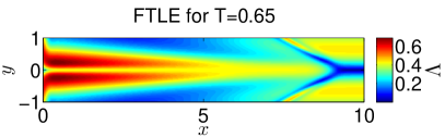
For instance, consider the incompressible flow

$$\begin{split}\dot{x}_{1}&=-x_{1}-s(t)\frac{x_{1}}{\cosh(x_{2})^{2}},\\ \dot{x}_{2}&=x_{2}+s(t)\tanh x_{2},\end{split}$$ (6)

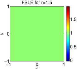
with the smooth function $s(t)$ again defined as in (5). This flow turns from a linear saddle into a nonlinear saddle gradually over the $[a,b]$ time interval. Therefore, computing the FSLE field $\sigma\left(x_{0};\delta_{0},r\right)$ from $t_{0}=0$ with any $r\leq\mathrm{e}^{a}$ gives

$$\sigma\left(x_{0};\delta_{0},r\right)=1,$$

for any choice of $x_{0}$ and $\delta_{0}$. Therefore, irrespective of the later transition of the flow from linear to nonlinear, a computation of the FSLE field will return $\sigma\equiv 1$ for a range of $r$ values. This range grows exponentially with the magnitude of $a$. Again, in case of an a priori unknown flow, one is unaware of flow structures and their temporal changes, and would precisely like to use the FSLE to obtain information about these unknown factors. Exploring all possible choices of the separation factor $r$ to obtain this information is clearly a tedious procedure.

By contrast, over a fixed time interval of observation $[0,t]$, the FTLE field $\Lambda_{t_{0}}^{t}(x_{0})$ will correctly assess the uniform linear separation rate for times up to $t=a$, then starts reflecting the developing inhomogeneity in separation by highlighting the stable manifold of the nonlinear saddle as a ridge for times $t>a$ (see Fig. 1).

Figure 1: FSLE and FTLE fields for the flow (6), with initial time $t_{0}=0$ and transition between $a=0.5$ and $b=0.6$. Left: FSLE field for $r=1.5$. Right: FTLE field for $T=1$.

3.3 Inherent jump-discontinuities of FSLE

While the FTLE is defined through the explicit formula (3), the FSLE field (1) relies on the separation time $\tau$ defined implicitly by Eq. (4). Solutions of such implicit equations generally admit discontinuities, and the FSLE field is no exception to this rule.

To illustrate this, we consider the system

$$\begin{split}\dot{x}_{1}&=-0.1\pi\sin\pi x_{1}\cos\pi x_{2},\\ \dot{x}_{2}&=0.1\pi\cos\pi x_{1}\sin\pi x_{2},\end{split}$$ (7)

a specific steady version of the double-gyre flow introduced by [29].

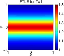
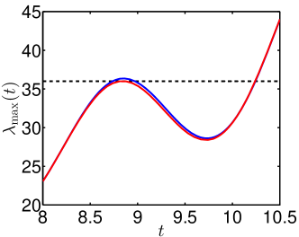
The left plot in Fig. 2 shows the FSLE field computed over one of the two gyres in the flow with separation factor $r=6$. Jump-discontinuities along a large family of curves are readily observed. These discontinuities become even more apparent in the middle plot, where we graph FSLE values along the line $x_{\textnormal{2,spec}}=0.48$ and $x_{1}\in\left[0,0.5\right]$.

Figure 2: Left: Lines of discontinuities in the FSLE field of the autonomous double gyre flow (7). Middle: A cross section of the discontinuities along the $x_{2,\textnormal{spec}}=0.48$ line. Right: The root cause of the jump-discontinuity at $x_{\textnormal{1,dis}}\approx 0.1583$: a tangency of the particle-separation history curve with the $r=6$ horizontal line.

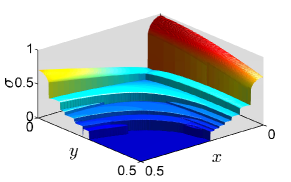
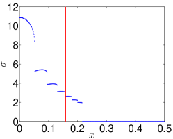
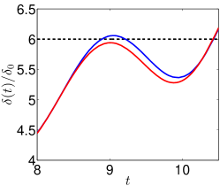
To identify the root cause behind such jump-discontinuities, we focus on one of the jump locations at $x_{\textnormal{1,dis}}\approx 0.1583$, indicated by the vertical line in the middle plot of Fig. 2 around which a discontinuity is observed. In the right plot of Fig. 2, we graph the time evolution of the largest relative particle separation $\delta(t,x_{0})/\delta_{0}$ for two nearby initial conditions, one on the left and one on the right of the $x_{\textnormal{1,dis}}\approx 0.1583$ line. This plot reveals a tangency between the $\delta(t;x_{\textnormal{1,dis}},x_{\textnormal{2,spec}})/\delta_{0}$ curve and the $r=6$ horizontal line. A consequence of this tangency is a sizable jump in the separation time (i.e., the smallest solution of the equation $\delta(\tau;x_{\textnormal{0}})/\delta_{0}=6$) as initial conditions are varied across $x_{\textnormal{1,dis}}$.

As we establish later in this paper, the above jump-discontinuities of the FSLE field are typical. They generically occur along families of codimension-one surfaces in the phase space of a nonlinear dynamical system (cf. Proposition 1).

3.4 Sensitivity of FSLE field with respect to temporal resolution

The presence of jump-discontinuities in the FSLE field may appear to be a strictly cosmetic issue. However, jumps in $\tau(x_{0};\delta_{0},r)$ result in a sensitivity of FSLE calculations with respect to the temporal resolution of the available flow data.

Indeed, the right subplot of Fig. 2 shows that under a course step size in $t$, the first crossing of the $\delta(t)/\delta_{0}=6$ line by the particle-separation history curve will be missed altogether for an open set of initial conditions. Instead of the correct separation time, a larger separation time will be recorded. The resulting error will typically be substantially larger than the time-step used in the computation.

LaCasce [21] has already observed that FSLE statistics show sensitivity with respect to the temporal resolution in the range of smaller $\delta_{0}$ scales. Such sensitivity can be gradually reduced for analytic and numerical model flows by selecting smaller and smaller time steps. Step-size reduction, however, is not an option for in situ observational flow data, which comes with a fixed (and typically course) temporal resolution [21].

By contrast, the FTLE field is everywhere continuous in the time parameter $t$ and the initial condition $x_{0}$. Furthermore, errors in an FTLE computation are typically of higher order with respect to the computational time step used in integrating the velocity field.

3.5 Spurious ridges of FSLE

Even in regions where the FSLE field is well-defined and continuous, FSLE ridges may signal false positives for repelling LCSs. Because of significant changes in the flow after the separation time is reached by key trajectories, the FSLE field may even produce such spurious ridges along trenches of the FTLE field.

As an example, consider a two-dimensional model for moving unsteady separation along a horizontal free-slip wall. The velocity field derives from the stream-function Hamiltonian

$$H(t,x)=-L\tanh(q_{2}x_{2})\tanh(q_{1}(x_{1}-at)),$$ (8)

where $L$ characterizes the strength of the separation; $q_{1}$ and $q_{2}$ control how localized the impact of separation is on the flow; and $a$ defines the horizontal speed at which the separation moves. The flow, therefore, becomes steady in a frame that moves horizontally with speed $a$.

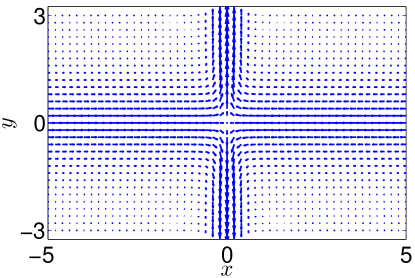
We fix the parameters $L=4$, $q_{1}=5$, $q_{2}=1$, and $a=10$, and choose the maximal length of observation time as $T=t-t_{0}=2$. For this choice of parameters, Fig. 3 shows the instantaneous velocity field for the model (8) at $t=0$.

Figure 3: Instantaneous velocity field for the moving separation flow (8).

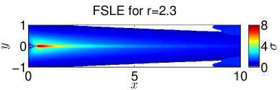
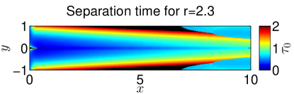
Selecting the separation factor as $r=2.3$, we observe in Fig. 4 (top left) an FSLE ridge along the $x_{1}$-axis, starting at about $0.3$. Since the separation point moves to the right, initial positions with larger and larger $x_{1}$-values experience separation at later and later times. As a result, the height of the FSLE ridge along the $x_{1}$ axis shows large variation. The separation-time plot in Fig. 4 (top right) highlights this further, indicating a separation-time valley with increasing bottom-height.

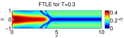
At the same time, by the localized nature of the separation, only a short segment of the $x_{1}$ axis will generate a ridge for the FTLE field for any choice of the integration time. This axis segment is the subset of initial conditions showing the most net separation over the time interval $T$. The rest of the $x_{1}$-axis is in fact an FTLE trench, as seen in Fig. 4 (bottom left). For longer integration times, an increasingly long subset of the $x_{1}$-axis becomes an FTLE valley, while two nearby FTLE ridges parallel approach it (Fig. 4, bottom right). Thus, one cannot even argue that the FSLE ridge can at least be continued into a nearby, unique FTLE ridge.

Figure 4: An FSLE ridge with large height-variation that does not correspond to an FTLE ridge. Top: FSLE and separation time distribution for the moving separation flow (8) with separation factor $r=2.3$. Note that the whole of the $x_{1}$ axis is a ridge for the FSLE field (left), as confirmed by the separation time field (right). Bottom: The FTLE fields for the integration times $T=0.3$ and $T=0.65$ admit a trench along most of the $x_{1}$ axis.

4 The Infinitesimal-Size Lyapunov Exponent (ISLE)

The examples of Section 3 illustrate the need to clarify the relationship between the FSLE and FTLE fields. The first challenge is that the FSLE is inherently linked to trajectory separation resulting from a finite-size initial perturbation $\delta_{0}$ to the initial condition $x_{0}$. By contrast, the FTLE describes the separation of trajectories starting infinitesimally close to $x_{0}$. To close this conceptual gap between the two quantities, we define the infinitesimal analog of FSLE by taking the $\delta_{0}\to 0$ limit in its definition.

Definition 1.

We define the Infinitesimal-Size Lyapunov Exponent (ISLE) as

$$\sigma_{0}\left(x_{0},r\right):=\lim_{\delta_{0}\to 0}\sigma\left(x_{0};\delta_{0},r\right).$$

For the FSLE field to provide a meaningful measure of trajectory separation at $x_{0}$, the ISLE field must be well-defined at $x_{0}$, i.e., its defining limit must exist. This is a prerequisite (albeit no guarantee) for the FSLE to detect hyperbolic LCSs reliably.

We now present a result on the existence, computation and relevance of the limit defining $\sigma_{0}.$ In formulating these results, we will use the infinitesimal analog $\tau_{0}(x_{0},r)$ of the finite-size separation time $\tau(x_{0};\delta_{0},r),$ defined as

$$\tau_{0}(x_{0},r):=\min\left\{\left|t-t_{0}\right|:\,\,t>t_{0},\,\,\lambda_{\max}\left(C{}_{t_{0}}^{t}(x_{0})\right)=r^{2}\right\}.$$

Theorem 1 (Relation of ISLE to FSLE).

Assume that $\lambda_{\max}\left(C_{t_{0}}^{t_{0}+\tau_{0}(x_{0},r)}(x_{0})\right)$ is a simple eigenvalue and

$$\partial_{t}\lambda_{\max}\left(C_{t_{0}}^{t_{0}+\tau_{0}(x_{0},r)}(x_{0})\right)\neq 0.$$ (9)

Then the following hold:

1. The ISLE field $\sigma_{0}\left(x_{0},r\right)$ is well-defined and $C^{2}$ at the point $x_{0}$, and can be computed as

   $$\sigma_{0}\left(x_{0},r\right)=\Lambda_{t_{0}}^{t_{0}+\tau_{0}\left(x_{0},r\right)}\left(x_{0}\right)=\frac{\log r}{\tau_{0}\left(x_{0},r\right)},$$ (10)

   with $\Lambda_{t_{0}}^{t}$ denoting the FTLE field defined in Eq. (3).

2. The FSLE field $\sigma\left(x_{0};\delta_{0},r\right)$ is also well-defined and $C^{2}$ at the point $x_{0}$, and satisfies

   $$\sigma\left(x_{0};\delta_{0},r\right)=\sigma_{0}\left(x_{0},r\right)+\mathcal{O}\left(\delta_{0}\right).$$ (11)

Proof.

See Appendix A. ∎

Remark 1.

Theorem 1 shows that computing the ISLE field, wherever it is well-defined, gives a close and smooth approximation to the FSLE field in the same domain. The advantage of the ISLE is that it is a pointwise indicator of finite-scale deformation, independent of the choice of initial grid size. This makes the ISLE field amenable to further mathematical analysis.

Remark 2.

As we show in Appendix A, condition (9) can also be written in the equivalent form

$$\left\langle DF_{t_{0}}^{t}(x_{0})e_{\max}\left(C_{t_{0}}^{t}(x_{0})\right),S\left(F_{t_{0}}^{t}(x_{0}),t\right)DF_{t_{0}}^{t}(x_{0})e_{\max}\left(C_{t_{0}}^{t}(x_{0})\right)\right\rangle|_{t=t_{0}+\tau_{0}(x_{0},r)}\neq 0,$$ (12)

where $DF_{t_{0}}^{t}(x_{0})$ denotes the flow gradient, and $S(x,t)=\frac{1}{2}\left[\nabla v(x,t)+\left(\nabla v(x,t)\right)^{T}\right]$ is the Eulerian rate-of-strain tensor. Formula (12) reveals that the ISLE and FSLE fields are well-defined and smooth at initial locations $x_{0}$ where the direction of largest Lagrangian strain is not mapped by the linearized flow map into a direction of zero instantaneous Eulerian strain.

The non-degeneracy condition (9) (or, equivalently, (12)) will fail along codimension-one surfaces of initial conditions in the phase space. The following proposition spells this fact out in more precise terms.

Proposition 1 (Degeneracy of FSLE along hypersurfaces).

The non-degeneracy condition (9) for the well-posedness of the FSLE field is generically violated along families of $(n-1)$-dimensional hypersurfaces in the flow domain $D\subset\mathbb{R}^{n}$. These hypersurfaces satisfy

$$\partial_{t}\lambda_{\max}\left(C_{t_{0}}^{t}(x_{0})\right)=0,\qquad\partial_{t}^{2}\lambda_{\max}\left(C_{t_{0}}^{t}(x_{0})\right)\neq 0,\qquad\partial_{x_{0}}\lambda_{\max}\left(C{}_{t_{0}}^{t}(x_{0})\right)\neq 0,$$ (13)

with the times $t=t_{0}+\tau_{0}(x_{0},r)$ substituted after the differentiations in (13).

Proof.

See Appendix A. ∎

Remark 3.

The hypersurfaces defined by formula (13) define locations of jump-discontinuities for the FSLE field. In a neighborhood of these surfaces, the FSLE will show sensitive dependence on the numerical step-size used in its computation. This generalizes our observations made in Section 3.4 from a specific two-dimensional, steady flow model to unsteady flows of arbitrary dimension. The resulting sensitivity with respect to the temporal resolution of the data will be particularly pronounced near hyperbolic LCSs, where the separation time $\tau(x_{0};\delta_{0},r)$ is low, and hence errors in its computation will cause significant errors in the FSLE.

Example 1.

In the double-gyre flow (7), the jump condition (13) holds along one-dimensional curves, as is apparent from Fig. 5. As a consequence, the ISLE field is not smooth along these locations, which results in jump-discontinuities in the FSLE field along crossing curves (cf. Fig. 2).

Figure 5: An occurrence of the first two FSLE jump-conditions in (13) along the $x_{2,\textnormal{spec}}=0.48$ line in the double-gyre flow (7). The third jump-condition in (13) is also satisfied, as the FTLE field does not have a stationary point at this location.

5 Ridges as invariant manifolds under the gradient flow

Ridges of the FTLE field are expected to signal hyperbolic LCSs, as initially proposed in [14] (see also [30] and [26]). While this expectation is often justified, more recent work has revealed that FTLE ridges may also produce both false negatives and false positives in LCS detection [16]. False positives can be filtered out by verifying further conditions along FTLE ridges [16, 13, 10, 20]. False negatives can be avoided by using more advanced, variational LCS methods that do not rely on FTLE ridges. These methods are supported by theorems, and render LCSs in a parametrized form, as solutions of differential equations [17, 9, 11].

By analogy with FTLE ridges, FSLE ridges have also been assumed to signal hyperbolic LCSs [19, 7, 23, 4, 22]. In view of the differences between the FSLE and FTLE surveyed in Section 3, a strict analogy between the ridges of the two fields cannot hold. Below we establish conditions under which an FSLE ridge does signal a nearby FTLE ridge, on which further hyperbolicity tests can be performed to ascertain the existence of a hyperbolic LCS in the flow.

Various ridge definitions are used in topology and visualization (cf. [8] for a general survey and [28] for an LCS-related review). Here we introduce a new definition that is particularly well-suited for ridge-continuation from one scalar field to another. Specifically, we view ridges of a scalar function $f(x)$ as codimension-one attracting invariant manifolds of the gradient dynamical system associated with $f(x)$. The following definition formalizes this view in mathematical terms, motivated by the FTLE-ridge extraction technique devised by [24].

Definition 2 (Ridge).

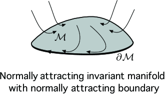
Let $f\colon\mathds{R}^{n}\to\mathds{R}$ be a class $C^{p}$ function with $p\geq 2$. Let $\mathcal{M}\subset\mathds{R}^{n}$ be a compact, codimension-one manifold, whose boundary $\partial\mathcal{M}$ is a compact, codimension-two manifold without boundary. We call $\mathcal{M}$ a ridge for the function $f$ if both $\mathcal{M}$ and $\partial\mathcal{M}$ are normally attracting invariant manifolds for the gradient dynamical system

$$\dot{x}=\nabla f(x).$$ (14)

By invariance of a manifold, we mean that trajectories of (14) starting in the manifold never leave it in either time direction. This implies that the gradient vector field $\nabla f(x)$ is contained in the tangent space $T_{x}\mathcal{M}$ at each point $x\in\mathcal{M}$. In addition, at each $x\in\partial\mathcal{M}$, we must also have $\nabla f(x)\in T_{x}\partial\mathcal{M}$.

By normal attraction for $\mathcal{M}$, we mean that contraction rates normal to $\mathcal{M}$ dominate any possible contraction rates along $\mathcal{M}$ [12]. Normal attraction for $\mathcal{\partial M}$ represents the same requirement, also implying that any contraction rate within $\mathcal{\partial M}$ must be weaker than contraction rates within $\mathcal{M}$ normal to its boundary $\mathcal{\partial M}$.

Sketched in the left plot of Fig. 6, the manifold forming the ridge $\mathcal{M}$ is robust under small perturbations to $f$ in the following sense.

Proposition 2 (Persistence of ridges).

A ridge in the sense of Definition 2 perturbs smoothly into a nearby $C^{1}$-close ridge under a small enough $C^{1}$ perturbation to the function $f(x).$

Proof.

See Appendix B. ∎

Figure 6: Left: Codimension-one, normally attracting invariant manifold with a normally attracting boundary for the gradient flow (14). Right: The geometry of the gradient flow (14) near a one-dimensional ridge $\mathcal{M}$.

The advantage of Definition 2 is that it guarantees robustness for the ridge based on powerful persistence results for normally hyperbolic invariant manifolds (see Proposition 2). Other available ridge definitions do not provide a well-defined set of conditions for ridge-persistence under changes in the underlying scalar field; only partial results exist for specific cases [6, 25].

On the other hand, verifying Definition 2 on a ridge-candidate set $\mathcal{M}$ involves the computation of Lyapunov-type numbers that guarantee normal hyperbolicity [12]. Computing these numbers can be laborious, requiring the numerical solution of trajectories of the gradient system (14) in $\mathcal{M}$.

This computational complexity is absent in the frequent case when all forward-time limit sets for trajectories of (14) in $\mathcal{M}$ are fixed points. In that case, it is sufficient to verify that the normal attraction rate to $\mathcal{M}$ and to $\mathcal{\partial M}$ at each fixed point dominates any potential tangential contraction rate within these manifolds at the fixed point. This is because Lyapunov-type numbers associated with a trajectory coincide with the Lyapunov-type numbers computed on the limit set of the trajectory [12].

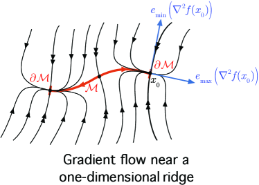
In the case of a one-dimensional ridge-candidate $\mathcal{M}$, all limit sets of system (14) within $\mathcal{M}$ are necessarily fixed points (see Fig. 6, right). Then, we obtain the following readily verifiable ridge criterion that does not require the numerical solution of the gradient system (14).

Proposition 3 (Existence of one-dimensional ridges).

Let $f\colon\mathds{R}^{2}\to\mathds{R}$ be a class $C^{2}$ function, and let $\mathcal{M}\subset\mathds{R}^{2}$ be a compact curve with boundary. Assume that

1. $\nabla f(x)\in T_{x}\mathcal{M}$ for all $x\in\mathcal{M}$;

2. $\nabla f(x)=0$ and $\lambda_{\mathrm{max}}\left(\nabla^{2}f(x)\right)<0$ for both points $x\in\mathcal{\partial M}$.

3. For all points $x_{0}\in\mathcal{M}$, where $\nabla f(x_{0})=0$, the Hessian $\nabla^{2}f(x_{0})$ has simple eigenvalues, with the smaller eigenvalue satisfying

   $$\lambda_{\min}\left(\nabla^{2}f(x_{0})\right) <0, e_{\min}\left(\nabla^{2}f(x_{0})\right) \perp T_{x_{0}}\mathcal{M}.$$

Then $\mathcal{M}$ is a ridge for the function $f$ in the sense of Definition 2.

Proof.

See Appendix B.∎

Remark 4.

As seen in Fig. 6 and as required by condition (2) of Proposition 3, a one-dimensional ridge in the sense of Definition 2 is necessarily a curve connecting two local maxima of a scalar field $f(x)$, and containing at least one more critical point of $\nabla f(x)$ in its interior.

Remark 5.

As noted by [28], requiring one of the eigenvectors of the Hessian $\nabla^{2}f(x)$ of a scalar field $f(x)$ to be parallel to a ridge $\mathcal{M}$ at all points $x\in\mathcal{M}$ leads to an over-constrained ridge definition. Our Definition 2 implies that one of the eigenvectors of $\nabla^{2}f(x_{0})$ is automatically parallel to $\mathcal{M}$ at any critical point $x_{0}$ of $f(x)$. This follows from the fact that $\mathcal{M}$ is an invariant manifold for the gradient flow $\dot{x}=\nabla f(x)$, and hence $T_{x_{0}}\mathcal{M}$ is necessarily an invariant subspace for the linearized gradient flow $\dot{y}=\nabla^{2}f(x_{0})y$ at any critical point $x_{0}\in\mathcal{M}$ of the function $f(x)$. Condition (iii) of Proposition 3 simply adds the requirement that the ridge-parallel eigenvector at $x_{0}$ should be the eigenvector corresponding to the smaller eigenvalue of the Hessian $\nabla^{2}f(x_{0})$.

6 When does an FSLE ridge signal a nearby FTLE ridge?

The following result establishes that an FSLE ridge indicates a nearby FTLE ridge, provided that the initial separation distance $\delta_{0}$ is small enough, and the ISLE separation times $\tau_{0}\left(x;r\right)$ along the FSLE ridge are close enough to a constant value in the $C^{2}$ norm.

Theorem 2 (Continuation of FSLE ridges into FTLE ridges).

Let $\mathcal{M}$ be a ridge of the FSLE field $\sigma\left(x;\delta_{0},r\right)$ in the sense of Definition 2. Assume that in a compact neighborhood $U$ of $\mathcal{M}$, we have

$$\partial_{t}\lambda_{\max}\left(C_{t_{0}}^{t_{0}+\tau_{0}(x,r)}(x)\right) \neq 0, \left\|\tau_{0}\left(x;r\right)-\bar{\tau}_{0}\right\|_{C^{2}} \leq\varepsilon, x \in U,$$ (15)

for appropriate constants $\bar{\tau}_{0}>0$ and $0\leq\varepsilon$, and with $\left\|\cdot\right\|_{C^{2}}$ referring to the $C^{2}$ norm. Then, for $\varepsilon,\delta_{0}$ sufficiently small, the FTLE field $\Lambda_{t_{0}}^{t_{0}+\bar{\tau}_{0}}\left(x\right)$ has a ridge $\mathcal{\bar{M}}$ that is $\mathcal{O}(\varepsilon,\delta_{0})$  $C^{1}$-close to $\mathcal{M}$.

Proof.

See Appendix B.∎

Remark 6.

Theorem 2 implies that there is an open set of $\bar{\tau}_{0}$ values for which the $\Lambda_{t_{0}}^{t_{0}+\bar{\tau}_{0}}\left(x\right)$ field will admit a nearby ridge. Indeed, small enough changes in the constant $\bar{\tau}_{0}$ will not affect the statement of the theorem.

Remark 7.

By formula (10), the second condition in (15) is equivalent to

$$\left\|\frac{1}{\bar{\sigma}}-\frac{1}{\sigma\left(x_{0},r\right)}\right\|_{C^{2}} \leq\frac{\varepsilon}{\log r}, \bar{\sigma} \coloneqq\frac{\log r}{\bar{\tau}_{0}}.$$

Therefore, one may equivalently require small enough variations in the reciprocal of ISLE field $\sigma\left(x_{0},r\right)$ in the $C^{2}$ norm within a compact neighborhood $U$ of the ridge $\mathcal{M}$. This in turn can be enforced by requiring small enough variations in the FSLE field along $\mathcal{M}$ by formula (11).

Remark 8.

By Fenichel’s results [12], the FTLE ridge is only guaranteed to be $\mathcal{O}(\varepsilon,\delta_{0})$ $C^{1}$-close to the original FSLE ridge. This means that the two ridges are pointwise close and their tangent spaces at these points are also close. Closeness of the curvatures of the two ridges, however, does not immediately follow in our setting.

Remark 9.

Assume that the FSLE field is of class $C^{s}$ with $s\geq 2$, and its ridge is a $C^{p}$ differentiable manifold with $p\geq 2$. Then the maximum degree of smoothness guaranteed for a nearby FTLE ridge will be

$$q=\min\left(s-1,p,\min_{x_{0}\in Z_{0}}\mathrm{Int}\left[\frac{\lambda_{\mathrm{min}}\left(\nabla^{2}f(x_{0})\right)}{\lambda_{\max}\left(\nabla^{2}f(x_{0})\right)}\right]\right)$$

by the theory of normally hyperbolic invariant manifolds [12]. Here we have used the set

$$Z_{0}=\left\{x_{0}\in\mathcal{M}:\,\,\nabla f(x_{0})=0,\,\,\lambda_{\mathrm{min}}\left(\nabla^{2}f(x_{0})\right)<\lambda_{\max}\left(\nabla^{2}f(x_{0})\right)<0\right\},$$

as well as the notation $\mathrm{Int\left[\cdot\right]}$ for the integer part of a positive real number. The quotient $\lambda_{\mathrm{min}}\left(\nabla^{2}f(x_{0})\right)/\lambda_{\max}\left(\nabla^{2}f(x_{0})\right)$ is just the Lyapunov-type number introduced by [12], computed at stationary values $x_{0}$ of $f$ along $\mathcal{M}$. The minimum of these Lyapunov-type numbers potentially limits the differentiability of the nearby FTLE ridge further, as seen from the formula defining $q$. In general, the larger the minimal Lyapunov-type number along the FSLE ridge, the more robust the ridge is under perturbations, i.e., the larger $\delta_{0}$ and $\epsilon$ can be selected in the statement of Theorem 2.

Example 2.

The moving separation example in Section 3.5 shows that large variations in the height of FSLE ridges do indeed result in the non-persistence of these ridges in the FTLE field. In this example, a large variation in $\tau_{0}$ is observed along the ISLE ridge defined by $x_{2}=0$, see Fig. 7. As a result, no constant $\bar{\tau}_{0}$ satisfying (15) can be selected for small values of $\varepsilon>0$.

Figure 7: The separation time distribution for the moving separation flow (8) with separation factor $r=2.3$.

Theorem 2 and Remark 9 show that FSLE ridges with small enough variations in their ISLE values in the $C^{2}$ norm, and with large enough transverse steepness at their peaks, give rise to nearby FTLE ridges. Example 2 shows that in flows violating this requirement, either no or several $C^{1}$-close FTLE ridges may exist. Therefore, the types of conditions required in Theorem 2 are indeed necessary for FSLE ridges to be meaningful in hyperbolic LCS detection, even though the constants arising in these conditions are not readily computable from our proof.

7 Inferring hyperbolic LCS from FSLE ridges

While select FSLE ridges signal the presence of nearby FTLE ridges by Theorem 2, this does not imply that there is always a corresponding hyperbolic LCS in the flow. Indeed, simple examples show that an FTLE ridge may simply indicate locations of locally maximal shear [15, 16].

More recent variational methods enable the direct extraction of hyperbolic LCSs as parametrized curves [9]. Further generalizations extend this computational advantage to parabolic and elliptic LCSs as well [17, 18].

These high-end detection techniques also require additional computational investment that ensures the accurate solution of differential equations derived from the eigenvector fields of the Cauchy–Green strain tensor. For a rough first assessment of hyperbolic LCSs, one may simply check additional criteria along FTLE ridges to conclude the existence of nearby hyperbolic LCSs. We refer the reader to [16, 13, 10, 20] for such criteria.

Conversely, given a spatial scale of interest, a preliminary FSLE analysis might be helpful in determining a relevant time scale of integration to be used in variational LCS methods.

8 Conclusions

Using the Infinitesimal-Size Lyapunov Exponent (ISLE), we have established a link between certain ridges of the FSLE field and those of the FTLE field. Specifically, FSLE ridges with moderate ISLE variations and high normal steepness at their peaks signal nearby FTLE ridges, as long as the time-derivative of the largest eigenvalue of the Cauchy-Green strain tensor is nonzero in a neighborhood of these FSLE ridges (cf. Theorem 2 and Remark 9). This nonzero derivative condition will, however, be violated along families of hypersurfaces in the phase space, over which the FSLE field admits jump-discontinuities.

Families of such FSLE jump-surfaces are generically present in any nonlinear flow (Proposition 1), creating sensitivity in FSLE computations with respect to the temporal resolution of the underlying flow data (cf. Remark 3). This sensitivity may even impact the accuracy of FSLE statistics, as has already been observed for float experiments in the ocean [21].

In addition to jump-discontinuities and the associated temporal sensitivity, we have also identified further disadvantages of the FSLE field in detecting Lagrangian coherence. These include ill-posedness for ranges of the separation parameter $r$, insensitivity to changes in the flow once the separation time $\tau$ is reached, and non-existence of nearby FTLE ridges in the case of FSLE ridges with substantial variation in their heights. We have illustrated all these issues with the FSLE in simple examples.

These findings suggest that the simplicity of computing FSLE comes at a price. If the objective is the accurate and threshold-free detection of hyperbolic LCSs, then more recent variational LCS techniques offer multiple advantages over FSLE-based coherence detection. While these variational techniques require a higher computational investment, they do provide a full and rigorous detection of all types of LCSs, including hyperbolic, parabolic, and elliptic LCSs [17, 3, 18]. This is to be contrasted with the substantial cost of varying two free parameters and with the remaining uncertainty in the results, if LCSs are to be inferred from the FSLE field without further mathematical analysis. On the upside, given a spatial scale of interest, FSLE may help in identifying the integration times to be used in variational LCS methods.

In summary, the use of the FSLE in hyperbolic LCS detection requires caution. Only flows with high temporal resolution and limited unsteadiness can be reliably analyzed. In addition, only ridges with moderate variations in their height and with high enough normal steepness at their peaks can be guaranteed to signal nearby LCSs. Even in such flows, the FSLE field will show sensitivity near hypersurfaces defined by the equation $\partial_{t}\lambda_{\max}\left(C_{t_{0}}^{t_{0}+\tau_{0}(x,r)}(x)\right)=0.$ This sensitivity is the highest near hyperbolic LCSs, as these lead to low values of the separation time, whose reciprocal values magnify errors in the FSLE field.

Acknowledgements

We thank Ronny Peikert for suggesting references on available persistence results for ridges. We also thank Joe LaCasce for stimulating discussions on Lagrangian statistics and their relation to the FSLE. We are grateful to Dan Blazevski and Mohammad Farazmand for their insights into the definition of ridges.

Appendix A Proof of Theorem 1, Remark 2 and Proposition 1

A.1 Proof of Theorem 1

The separation time $\tau(x_{0};\delta_{0},r)$ at the initial condition $x_{0}$ is the smallest positive solution of the equation

$$\begin{split}r^{2}\delta_{0}^{2}&=\left|F_{t_{0}}^{t_{0}+\tau}(y_{0})-F_{t_{0}}^{t_{0}+\tau}(x_{0})\right|^{2}\\ &=\left|DF_{t_{0}}^{t_{0}+\tau}(x_{0})\left(y_{0}-x_{0}\right)+\mathcal{O}\left(\left|y_{0}-x_{0}\right|^{2}\right)\right|^{2}\\ &=\delta_{0}^{2}\left\langle e\left(x_{0}\right),\left[DF_{t_{0}}^{t_{0}+\tau}(x_{0})\right]^{T}DF_{t_{0}}^{t_{0}+\tau}(x_{0})e\left(x_{0}\right)\right\rangle+\mathcal{O}\left(\delta_{0}^{3}\right)\\ &=\delta_{0}^{2}\left\langle e\left(x_{0}\right),C_{t_{0}}^{t_{0}+\tau}(x_{0})e\left(x_{0}\right)\right\rangle+\mathcal{O}\left(\delta_{0}^{3}\right),\end{split}$$ (16)

where

$$e\left(x_{0}\right)=\frac{y_{0}-x_{0}}{\left|y_{0}-x_{0}\right|},$$

is the unit vector pointing from $x_{0}$ towards $y_{0}$. Dividing (16) by $\delta_{0}^{2}$, we obtain

$$\left\langle e\left(x_{0}\right),C_{t_{0}}^{t_{0}+\tau}(x_{0})e\left(x_{0}\right)\right\rangle+\mathcal{O}\left(\delta_{0}\right)=r^{2},$$ (17)

which is equivalent to (16) for all $\delta_{0}>0$.

By continuity of all quantities involved in (17), the limit $\tau(x_{0},r)=\lim_{\delta_{0}\to 0}\tau(x_{0};\delta_{0},r)$ must coincide with the minimal solution $\tau$ of the equation

$$\left\langle e\left(x_{0}\right),C_{t_{0}}^{t_{0}+\tau}(x_{0})e\left(x_{0}\right)\right\rangle=r^{2}.$$ (18)

To explore the solvability of the limiting equation (18), recall that the Cauchy–Green strain tensor $C_{t_{0}}^{t_{0}+\tau}(x_{0})$ is symmetric, positive definite, and satisfies $C_{t_{0}}^{t_{0}}(x_{0})=I$, with $I$ denoting the identity matrix. Consequently, $\tau_{0}(x_{0},r)\coloneqq\tau(x_{0};0,r)$ is the smallest positive solution of (18) if $e\left(x_{0}\right)$ is chosen as the unit dominant eigenvector $e_{\max}\left(C_{t_{0}}^{t_{0}+\tau_{0}(x_{0},r)}(x_{0})\right)$ of the associated Cauchy–Green strain tensor. In that case, an equivalent equation for the smallest positive root of (18) is given by

$$\lambda_{\max}\left(C_{t_{0}}^{t_{0}+\tau_{0}(x_{0},r)}(x_{0})\right)=r^{2},$$ (19)

which implies the formula (10), and hence proves statement (i) of Theorem 1 with the exception of the claim of $C^{2}$ smoothness.

To prove statement (ii) of Theorem 1 and the $C^{2}$ smoothness in statement (i), we want to continue the solution of equation (17) smoothly from $\delta_{0}=0$ to $\delta_{0}>0$ values. By the implicit function theorem, this continuation requires precisely condition (9) to hold. Also, the continued solution will be $C^{2}$ smooth by the implicit function theorem, given that the right-hand side of (2), and hence the flow map, are assumed to be $C^{3}$ smooth. Consequently, statement (ii) of Theorem 1 follows.

A.2 Proof of Remark 2

Observe that the derivative in the non-degeneracy condition (9) can be computed as

$$\partial_{\tau}\lambda_{\max}\left(C_{t_{0}}^{t_{0}+\tau}(x_{0})\right) =\partial_{\tau}\left\langle e_{\mathrm{max}}\left(C_{t_{0}}^{t_{0}+\tau}(x_{0})\right),C_{t_{0}}^{t_{0}+\tau}(x_{0})e_{\mathrm{max}}\left(C_{t_{0}}^{t_{0}+\tau}(x_{0})\right)\right\rangle$$

$$=\left\langle e_{\mathrm{max}}\left(C_{t_{0}}^{t_{0}+\tau}(x_{0})\right),\partial_{\tau}C_{t_{0}}^{t_{0}+\tau}(x_{0})e_{\mathrm{max}}\left(C_{t_{0}}^{t_{0}+\tau}(x_{0})\right)\right\rangle,$$ (20)

where we have used the fact that

$$\partial_{\tau}e_{\mathrm{max}}\left(C_{t_{0}}^{t_{0}+\tau}(x_{0})\right)\perp e_{\mathrm{max}}\left(C_{t_{0}}^{t_{0}+\tau}(x_{0})\right),$$

given that $\left|e_{\mathrm{max}}\left(C_{t_{0}}^{t_{0}+\tau}(x_{0})\right)\right|\equiv 1.$ Furthermore, we have

$$\partial_{\tau}C_{t_{0}}^{t_{0}+\tau}(x_{0})\bigr{|}{}_{\tau_{0}(x_{0},r)}=\left[\partial_{\tau}\left(DF_{t_{0}}^{t_{0}+\tau}(x_{0})\right)^{T}DF_{t_{0}}^{t_{0}+\tau}(x_{0})+\right.\\ \left.\left.+\left(DF_{t_{0}}^{t_{0}+\tau}(x_{0})\right)^{T}\partial_{\tau}\left(DF_{t_{0}}^{t_{0}+\tau}(x_{0})\right)\right]\right|{}_{\tau_{0}(x_{0},r)}.$$ (21)

We recall that the deformation gradient $DF_{t_{0}}^{t_{0}+\tau}(x_{0})$ satisfies the equations of variation

$$\partial_{\tau}\left(DF_{t_{0}}^{t_{0}+\tau}(x_{0})\right)=\partial_{x}v\left(F_{t_{0}}^{t_{0}+\tau}(x_{0}),\tau\right)DF_{t_{0}}^{t_{0}+\tau}(x_{0}).$$ (22)

Substituting expression (22) into (21), then the resulting equation into (20) shows that conditions (9) and (12) are indeed equivalent, as claimed in Remark 2.

A.3 Proof of Proposition 1

First, note that points violating the conditions for the well-posedness of the FSLE satisfy the two scalar equations

$$\lambda_{\max}\left(C{}_{t_{0}}^{t_{0}+\tau_{0}}(x_{0})\right)-r^{2} = 0,$$ (23)

$$\partial_{t}\lambda_{\max}\left(C_{t_{0}}^{t_{0}+\tau_{0}}(x_{0})\right) = 0.$$ (24)

Assume that an isolated solution $(\bar{\tau}_{0},\bar{x}_{0})$ exists to this system of equations, such that $\bar{\tau}_{0}>0$ is also the minimal solution of (23) for $\bar{x}_{0}$. Then, by definition, $\bar{\tau}_{0}(\bar{x}_{0})$ is the separation time for the initial condition $\bar{x}_{0}$ with separation factor $r$. Furthermore, this separation time violates the non-degeneracy condition (9). Since being a minimal solution is an open property and (23) is continuous in its arguments, any solutions $(\tau_{0},x_{0})$ of system (23)-(24) close enough to $(\bar{\tau}_{0},\bar{x}_{0})$ will also define a separation time and its corresponding location.

We would like to argue that a set of nearby solutions to equation (9) generically exists and forms a smooth, $(n-1)$-dimensional surface in the space of the $(\tau_{0},x_{0})$ variables. To this end, we let $x_{0}^{1}$ denote the first coordinate of $x_{0}$ and let $x_{0}^{(n-1)}$ denote the remaining $(n-1)$ coordinates of $x_{0}$, so that $x_{0}=(x_{0}^{1},x_{0}^{(n-1)})$. We seek to establish that near the solution $(\bar{\tau}_{0},\bar{x}_{0}^{1},\bar{x}_{0}^{(n-1)})$, the system of equation (23)-(24) will continue to admit a smooth solution of the form

$$(\tau_{0},x_{0}^{1})=(\bar{\tau}_{0},\bar{x}_{0}^{1})+h\left(x_{0}^{(n-1)}-\bar{x}_{0}^{(n-1)}\right),$$

where $h\colon U\subset\mathbb{R}^{n-1}\to\mathbb{R}^{2}$ is a smooth function with $h(0)=0$, defined in a neighborhood $U$ of the origin $0\in\mathbb{R}^{n-1}$. This follows from a direct application of the implicit function theorem to the equations (23)-(24), provided that

$$\left.\det\begin{pmatrix}\partial_{t}\lambda_{\max}\left(C{}_{t_{0}}^{t}(x_{0})\right)&\partial_{x_{0}^{1}}\lambda_{\max}\left(C{}_{t_{0}}^{t}(x_{0})\right)\\ \partial_{t}^{2}\lambda_{\max}\left(C_{t_{0}}^{t}(x_{0})\right)&\partial_{x_{0}^{1}}\partial_{t}\lambda_{\max}\left(C_{t_{0}}^{t}(x_{0})\right)\end{pmatrix}\right|_{t=t_{0}+\bar{\tau}_{0},x_{0}=\bar{x}_{0}}\neq 0.$$ (25)

By equation (24), the first diagonal entry of the matrix in (25) is zero, and hence (25) is equivalent to

$$\partial_{t}^{2}\lambda_{\max}\left(C_{t_{0}}^{t}(x_{0})\right)\partial_{x_{0}^{1}}\lambda_{\max}\left(C{}_{t_{0}}^{t}(x_{0})\right)\neq 0,\qquad t=t_{0}+\bar{\tau}_{0},\quad x_{0}=\bar{x}_{0}.$$

This latter condition is satisfied as long as (1) $\lambda_{\max}\left(C_{t_{0}}^{t}(\bar{x}_{0})\right)$ has a non-degenerate temporal maximum at the degenerate separation time $\bar{\tau}_{0}(\bar{x}_{0})$ separation, and (2) the maximal eigenvalue $\lambda_{\max}\left(C{}_{t_{0}}^{t}(x_{0})\right)$ varies strictly in the $x_{0}^{1}$ direction. Condition (1) holds by the first inequality in (13). Condition (2) can always be satisfied by a possible reordering of the coordinates of the vector $x_{0}$, given that the second inequality in (13) is assumed to hold.

Appendix B Proof of Proposition 2, Proposition 3, and Theorem 2

B.1 Proof of Proposition 2

Elements of this flow geometry sketched in Fig. 6 were studied by Fenichel [12], who established general persistence results for compact, normally hyperbolic invariant manifolds under small perturbations. These results imply that $\mathcal{\partial M}$ smoothly and uniquely persists in the form of a nearby attracting, invariant manifold $\overline{\partial\mathcal{M}}$ under small perturbations. Furthermore, $\mathcal{M}$ can be slightly enlarged into a normally attracting, inflowing invariant manifold $\mathcal{N}$ beyond its boundary. (An inflowing invariant manifold is a manifold tangent to the underlying vector field, such that the vector field points strictly inwards along the boundary of the manifold.) By Fenichel [12], such a manifold $\mathcal{N}$ also persists smoothly (but typically not uniquely) as an attracting, inflowing invariant manifold $\overline{\mathcal{N}}$.

Now $\overline{\partial\mathcal{M}}$ necessarily lies in the domain of attraction of $\overline{\mathcal{N}}$, which is only possible if $\overline{\partial\mathcal{M}}\subset\overline{\mathcal{N}}$. Then the closure of the interior of $\overline{\partial\mathcal{M}}$ within $\overline{\mathcal{N}}$, which we denote by $\overline{\mathcal{M}}$, is a codimension-one, normally attracting invariant manifold such that its boundary satisfies $\partial\overline{\mathcal{M}}=\overline{\partial\mathcal{M}}$. Consequently, the original manifold $\mathcal{M}$ has smoothly perturbed into $\overline{\mathcal{M}}$ under small enough perturbations, as claimed.

B.2 Proof of Proposition 3

Condition (1) of Proposition 3 ensures that the codimension-one manifold $\mathcal{M}$ is invariant under the flow of (14). Condition (2) ensures that the boundary points (which are necessarily fixed points by the invariance of $\mathcal{M}$) are attracting along $\mathcal{M}$. Condition (3) ensures that at the fixed points of the gradient flow (14) contained in $\mathcal{M}$, the contraction rates normal to $\mathcal{M}$ dominate any possible contraction rate inside $\mathcal{M}$. Since the asymptotic normal attracting properties of trajectories coincide with those of their limit sets [12], normal attraction for the whole of $\mathcal{M}\subset\mathds{R}^{2}$ follows from the fact that normal attraction holds at all fixed points of (14) inside $\mathcal{M}$.

B.3 Proof of Theorem 2

The first condition in (15) ensures that both the FSLE and ISLE fields remain well-defined and smooth in the whole compact neighborhood $U$. Then, by the second condition in (15), we can write

$$\sigma\left(x;\delta_{0},r\right) =\sigma_{0}\left(x;r\right)+\mathcal{O}_{2}(\delta_{0})=\Lambda_{t_{0}}^{t_{0}+\tau_{0}(x_{0},r)}\left(x\right)+\mathcal{O}_{2}(\delta_{0})=\Lambda_{t_{0}}^{t_{0}+\bar{\tau}_{0}+\mathcal{O}(\varepsilon)}\left(x\right)+\mathcal{O}_{2}(\delta_{0})$$

$$=\Lambda_{t_{0}}^{t_{0}+\bar{\tau}_{0}}\left(x\right)+\mathcal{O}_{2}(\varepsilon,\delta_{0}),$$

where the $\mathcal{O}_{2}(\delta_{0})$ and $\mathcal{O}_{2}(\varepsilon,\delta_{0})$ terms denote a small, $C^{2}$ perturbation to the function $\Lambda_{t_{0}}^{t_{0}+\bar{\tau}_{0}}\left(x\right)$. As a result, we have

$$\dot{x}=\nabla\Lambda_{t_{0}}^{t_{0}+\bar{\tau}_{0}}\left(x\right)=\partial_{x}\sigma\left(x;\delta_{0},r\right)+\mathcal{O}_{1}(\varepsilon,\delta_{0}),$$ (26)

in the compact neighborhood $U$ of $\mathcal{M}$, with $\mathcal{O}_{1}(\varepsilon,\delta_{0})$ denoting terms that are $\mathcal{O}(\varepsilon,\delta_{0})$ $C^{1}$-small.

Then, by Proposition 2, the dynamical system (26) admits a ridge $\widetilde{\mathcal{M}}$ in the sense of Definition 2, which is $\mathcal{O}(\varepsilon,\delta_{0})$ $C^{1}$-close to $\mathcal{M}$, as claimed.

References

- [1] V. Artale, G. Boffetta, A. Celani, M. Cencini, and A. Vulpiani. Dispersion of passive tracers in closed basins: Beyond the diffusion coefficient. Phys. Fluids, 9(11):3162–3171, 1997.
- [2] E Aurell, G Boffetta, A Crisanti, G Paladin, and A Vulpiani. Predictability in the large: an extension of the concept of Lyapunov exponent. Journal of Physics A, 30(1):1, 1997.
- [3] F. J. Beron Vera, Y. Wang, M. J. Olascoaga, G. J. Goni, and G. Haller. Objective detection of oceanic eddies and the Agulhas leakage. Journal of Physical Oceanography, 43(7):1426–1438, 2013.
- [4] J. H. Bettencourt, C. López, and E. Hernández García. Characterization of coherent structures in three-dimensional turbulent flows using the finite-size Lyapunov exponent. Journal of Physics A: Mathematical and Theoretical, 46(25):254022, 2013.
- [5] M. Cencini and A. Vulpiani. Finite size Lyapunov exponent: review on applications. Journal of Physics A: Mathematical and Theoretical, 46(25):254019, 2013.
- [6] J. Damon. Properties of Ridges and Cores for Two-Dimensional Images. J. Math. Imaging Vision, 10(2):163–174, 1999.
- [7] F. d’Ovidio, V. Fernández, E. Hernández García, and C. López. Mixing structures in the Mediterranean Sea from finite-size Lyapunov exponents. Geophys. Res. Lett., 31(17):L17203, 2004.
- [8] D. Eberly, R. Gardner, B. Morse, S. Pizer, and C. Scharlach. Ridges for image analysis. J. Math. Imaging Vis., 4:353–373, 1994.
- [9] M. Farazmand and G. Haller. Computing Lagrangian coherent structures from their variational theory. Chaos, 22(1):013128, 2012.
- [10] M. Farazmand and G. Haller. Erratum and addendum to “A variational theory of hyperbolic Lagrangian coherent structures [Physica D 240 (2011) 574–598]”. Physica D, 241(4):439–441, 2012.
- [11] M. Farazmand and G. Haller. Attracting and repelling Lagrangian coherent structures from a single computation. Chaos, 23(2):023101, 2013.
- [12] N. Fenichel. Persistence and Smoothness of Invariant Manifolds for Flows. Indiana Univ. Math. J., 21(3):193–226, 1971.
- [13] G. Haller. Finding finite-time invariant manifolds in two-dimensional velocity fields. Chaos, 10(1):99–108, 2000.
- [14] G. Haller. Distinguished material surfaces and coherent structures in three-dimensional fluid flows. Physica D, 149(4):248–277, 2001.
- [15] G. Haller. Lagrangian coherent structures from approximate velocity data. Physics of Fluids, 14(6):1851–1861, 2002.
- [16] G. Haller. A variational theory of hyperbolic Lagrangian Coherent Structures. Physica D, 240(7):574–598, 2011.
- [17] G. Haller and F. J. Beron Vera. Geodesic theory of transport barriers in two-dimensional flows. Physica D, 241(20):1680–1702, 2012.
- [18] G. Haller and F. J. Beron Vera. Coherent Lagrangian vortices: The black holes of turbulence. Journal of Fluid Mechanics, 731(R4), 2013.
- [19] B. Joseph and B. Legras. Relation between Kinematic Boundaries, Stirring, and Barriers for the Antarctic Polar Vortex. J. Atmos. Sci., 59(7):1198–1212, 2002.
- [20] D. Karrasch. Comment on “A variational theory of hyperbolic Lagrangian Coherent Structures, Physica D 240 (2011) 574–598”. Physica D, 241(17):1470–1473, 2012.
- [21] J.H. LaCasce. Statistics from Lagrangian observations. Progress in Oceanography, 77(1):1 – 29, 2008.
- [22] Y.-C. Lai and T. Tél. Transient Chaos - Complex Dynamics on Finite Time Scales, volume 173 of Applied Mathematical Sciences. Springer, 2011.
- [23] Y. Lehahn, F. d’Ovidio, M. Lévy, and E. Heifetz. Stirring of the northeast Atlantic spring bloom: A Lagrangian analysis based on multisatellite data. J. Geophys. Res., 112:C08005, 2007.
- [24] M. Mathur, G. Haller, T. Peacock, J. E. Ruppert Felsot, and H. L. Swinney. Uncovering the Lagrangian Skeleton of Turbulence. Phys. Rev. Lett., 98(14):144502, 2007.
- [25] G. Norgard and P.-T. Bremer. Ridge-Valley graphs: Combinatorial ridge detection using Jacobi sets. Comput. Aided Geom. Design, 30(6):597 – 608, 2013.
- [26] T. Peacock and G. Haller. Lagrangian coherent structures: The hidden skeleton of fluid flows. Physics Today, 66(2):41–47, 2013.
- [27] R. Peikert, A. Pobitzer, F. Sadlo, and B. Schindler. A Comparison of Finite-Time and Finite-Size Lyapunov Exponents. In P-T. Bremer, I. Hotz, V. Pascucci, and R. Peikert, editors, Topological Methods in Data Analysis and Visualization III. Springer, 2014. to appear.
- [28] B. Schindler, R. Peikert, R. Fuchs, and H. Theisel. Ridge Concepts for the Visualization of Lagrangian Coherent Structures. In R. Peikert, H. Hauser, H. Carr, and R. Fuchs, editors, Topological Methods in Data Analysis and Visualization II, pages 221–236. Springer, 2012.
- [29] S. C. Shadden, F. Lekien, and J. E. Marsden. Definition and properties of Lagrangian coherent structures from finite-time Lyapunov exponents in two-dimensional aperiodic flows. Physica D, 212(3-4):271–304, 2005.
- [30] Shawn C. Shadden. Lagrangian Coherent Structures. In R. Grigoriev, editor, Transport and Mixing in Laminar Flows, pages 59–89. Wiley, 2011.