Multi-dimensional Parametric Mincuts for Constrained MAP Inference

Abstract

In this paper, we propose novel algorithms for inferring the Maximum a Posteriori (MAP) solution of discrete pairwise random field models under multiple constraints. We show how this constrained discrete optimization problem can be formulated as a multi-dimensional parametric mincut problem via its Lagrangian dual, and prove that our algorithm isolates all constraint instances for which the problem can be solved exactly. These multiple solutions enable us to even deal with ‘soft constraints’ (higher order penalty functions). Moreover, we propose two practical variants of our algorithm to solve problems with hard constraints. We also show how our method can be applied to solve various constrained discrete optimization problems such as submodular minimization and shortest path computation. Experimental evaluation using the foreground-background image segmentation problem with statistic constraints reveals that our method is faster and its results are closer to the ground truth labellings compared with the popular continuous relaxation based methods.

1 Introduction

Markov Random Fields (MRF) is an undirected graphical model, which has been extensively studied and used in various fields, including statistical physics [11], and computer vision [19]. It represents interdependency of discrete random variables as a graph over which a probabilistic space is defined. Computing the solution which has the maximum probability under the random field, or Maximum a Posteriori (MAP) inference is NP-hard in general. However, a number of subclasses of MRFs have been isolated for which the problem can be solved in polynomial time [2]. Further, a number of heuristics or approximation algorithms based on belief propagation [34], tree reweighted message passing [33], and graph-cut [3] have also been proposed for the problem. Such algorithms are widely used for various problems in machine learning and computer vision [38, 17]. Since MAP inference in an MRF is equivalent to minimizing the corresponding energy function, in what follows, we will explain these problems in terms of energy minimization.

In many real world problems, the values of certain statistics of the desired solution may be available as prior knowledge. For instance, in the case of foreground-background image segmentation, we may know the approximate shape and/or size of the object being segmented, and thus might want to find the most probable segmentation that has a particular area (number of foreground pixels) and boundary length (number of discontinuities). Another example is community detection in a network [8] where we may know the number of nodes belonging to each community. Such scenarios result in constraints in the solution space, and MAP inference becomes a constrained energy minimization problem, which is generally NP-hard even if the unconstrained version is polynomial time solvable.

Energy minimization under the above-mentioned statistics constraints results in a challenging optimization problem. However, recent work in computer vision has shown that this problem can be handled efficiently using the parametric mincuts [14] which allow simultaneous computation of exact solutions for some constraint instances. Although the parametric mincuts provide a general framework to deal with constrained energy minimization, they can only handle one linear equality constraint.

For minimizing energy functions under multiple constraints, a number of continuous relaxation based methods have been proposed in the literature. For instance, linear relaxation approaches were adopted to handle bounding-box and connectivity constraints defined on the labelling [18, 24]. Further, Klodt and Cremers [12] proposed a convex relaxation framework to deal with moment constraints. Continuous relaxation based methods have also been used for constrained discrete optimization, and can handle multiple inequality constraints. All the above-mentioned methods suffer from following basic limitations: they only handle linear constraints, and the solution involves rounding of the solution of the relaxed problem which may introduce large errors.

1.1 Our contribution

In this paper we show how the constrained discrete optimization problem associated with constrained MAP inference can be formulated as a multi-dimensional parametric mincut problem via its Lagrangian dual, and propose an algorithm that isolates all constraint instances for which the problem can be solved exactly. This leads to densely many minimizers, each of which is, optimal under distinct constraint instance. These minimizers can be used to compute good approximate solutions of problems with soft constraints (enforced with a higher order term in the energy).

Our algorithm works by exploiting the Lagrangian dual of the minimization problem, and requires an oracle which can compute values of the Lagrangian dual efficiently. A graph-cut algorithm [3] is a popular example of such an oracle. In fact, our algorithm generalizes the (one-dimensional) parametric mincuts [5, 14] to multiple-dimensions. In contrast to the parametric mincuts [5], our algorithm can deal with multiple constraints simultaneously, including some non-linear constraints (as we show in the paper). This extension allows our algorithm to be used as a technique for multi-dimensional sampling e.g. to obtain different segmentation results for image segmentation as done in [4].

We propose two variants of our algorithm to efficiently deal with the problem of performing MAP Inference under hard constraints. The first variant computes the maximum of the dual and outputs its corresponding primal solution as an approximation of the constrained minimization. The primal is computed using selective oracle calls, leading to fast computation time. The other variant combines the first variant with our multi-dimensional parametric mincuts algorithm to deal with problems with soft-constraints, which allows to find a solution closer to a desired one via additional search.

Our method is quite general and can be applied to any constrained discrete optimization problems whose Lagrangian dual value is efficiently computable. Examples include submodular function minimization with constraints such as the balanced minimum cut problem, and constrained shortest path problems. Further, in contrast to traditional continuous relaxation based methods, our technique can easily handle complicated soft constraints.

In Section 5, we demonstrate that our algorithms compute solutions very close to the ground truth compared with these continuous relaxation based methods on the foreground-background image segmentation problem.

1.2 Related work

A number of methods have been proposed to obtain better labelling solutions by inferring the MAP solution from a restricted domain of solutions which satisfy some constraints. Among them, solutions to image labelling problems which have a particular distribution of labels [36] or satisfy a topological property like connectivity [32] have been widely studied.

More specifically, for the problem of foreground-background image segmentation, most probable segmentations under the label count constraint have been shown to be closer to the ground truth [14, 20]. Another example is the silhouette constraint which has been used for the problem of 3D reconstruction [13, 29]. This constraint ensured that a ray emanating from any silhouette pixel must pass through at least one voxel which belongs to the ‘object’.

Recently, dual decomposition has been proposed for constrained MAP inference [7, 37]. Gupta et al. [7] dealt with cardinality-based clique potentials and developed both exact and approximate algorithms. Also Woodford et al. [37] studied a problem involving marginal statistics such as the area constraint especially with convex penalties, and showed that the proposed method improves quality of solutions for various computer vision problems.

MAP inference under constraints are also applied to combinatorial optimization such as the balanced metric labelling. For this problem, Naor and Schwartz [23] obtained an $O(\tfrac{\ln{n}}{\epsilon})$-approximate algorithm where each label is assigned to at most $\min\left[\tfrac{O(\ln{k})}{1-\epsilon},\ell+1\right](1+\epsilon)\ell$ variables/nodes.

2 Setup and preliminaries

2.1 Energy minimization

Markov Random Fields (MRF) defined on a graph $G=(V,E)$ is a probability distribution where every vertex $u\in V$ has a corresponding random variable $x_{u}$ taking a value from the finite label set ${\mathcal{L}}$. The probability distribution is defined as $\Pr(x)\propto\exp(-f(x))$ where $x=(x_{u})$, and the corresponding energy function $f$ is in the following form:

$$f(x)=\sum_{c\in{\mathcal{C}}_{G}}\phi_{c}(x_{c}),$$ (1)

where ${\mathcal{C}}_{G}$ is the set of cliques in $G$ and $\phi_{c}$ is a potential defined over the clique $c$. The MAP problem is to find an assignment $x^{*}\in{\mathcal{L}}^{|V|}$ which has the maximum probability, and is equivalent to minimizing the corresponding energy function $f$. In general it is NP-hard to minimize $f$, but it is known that if $f$ is submodular, it can be minimized in polynomial time. Especially, if $f$ is a pairwise submodular energy function defined on binary variables, which considers only cliques of size up to $2$, i.e.

$$f(x)=\sum_{u\in V}\phi_{u}(x_{u})+\sum_{(u,v)\in E}\phi_{uv}(x_{u},x_{v}),$$ (2)

it can be efficiently minimized by solving a equivalent st-mincut problem [15]. Such $f$ is widely used in machine learning and computer vision [9, 20].

2.2 Energy minimization with constraints

Energy minimization with constraints is to compute the solution $x^{*}$ minimizing an energy function among $x$’s satisfying given constraints. A typical example of constraints is the label count constraint $\sum_{i}x_{i}=b$ where $x_{i}\in\{0,1\}$.

In this paper, we consider the following energy minimization with multiple constraints.

$$\min_{x\in\{0,1\}^{n}}\left\{f(x):h_{i}(x)=b_{i},~{}1\leq i\leq m\right\},$$ (3)

where $x\in\{0,1\}^{n}$, $m$ is a constant, and for $1\leq i\leq m$, $h_{i}:\{0,1\}^{n}\rightarrow{\mathbb{R}}$ and $b_{i}\in{\mathbb{R}}$. In (3), each constraint $h_{i}(x)=b_{i}$ encodes distinct prior knowledge on a desired solution. For convenience, we denote $\left(h_{1}(x),\ldots,h_{m}(x)\right)$ by $H(x)$.

Let us consider the following Lagrangian dual $g:{\mathbb{R}}^{m}\rightarrow{\mathbb{R}}$ of $f$, which is widely used for discrete optimization [16, 30].

$$g(\lambda)=\min_{x\in\{0,1\}^{n}}L(x,\lambda),$$ (4)

where

$$L(x,\lambda)=f(x)+\lambda^{T}(H(x)-b).$$ (5)

Note that $g$ is defined over a continuous space while $f$ is defined over a discrete space. As in the continuous minimization, maximizing $g$ over $\lambda\in{\mathbb{R}}^{m}$ provides a lower bound for (3). Now we define the characteristic set, which is the collection of minimizers of (5) over all $\lambda\in{\mathbb{R}}^{m}$.

Definition 1 (Characteristic Set).

The Characteristic Set is defined by

$$\chi_{g}=\bigcup_{\lambda\in{\mathbb{R}}^{m}}\operatorname*{argmin}_{x\in\{0,1\}^{n}}L(x,\lambda).$$ (6)

Lemma 1.

Let $x^{*}\in\chi_{g}$ and $b^{*}=H(x^{*})$. Then $f(x^{*})=\min_{x\in\{0,1\}^{n}}\left\{f(x):H(x)\right.$
$\left.=b^{*}\right\}$ [6].

Proof.

Suppose that $\hat{x}$ satisfies that $H(\hat{x})=b^{*}$. It implies $\lambda^{T}(H(\hat{x})-b^{*})=\lambda^{T}(H(x^{*})-b^{*})$ for any $\lambda\in{\mathbb{R}}^{m}$. Since $x^{*}\in\chi_{g}$, $L(x^{*},\lambda)\leq L(\hat{x},\lambda)$ for some $\lambda\in{\mathbb{R}}^{m}$. Thus, from (5), $f(x^{*})\leq f(\hat{x})$. ∎

In this paper, we develop a novel algorithm to compute the characteristic set $\chi_{g}$. We will show that if the dual $g(\lambda)$ is efficiently computable for any fixed $\lambda\in{\mathbb{R}}^{m}$, for example, when $L(x,\lambda)$ is submodular on $x$, our algorithm computes $\chi_{g}$ by evaluating $g(\lambda)$ for $poly(|\chi_{g}|)$ number of $\lambda\in{\mathbb{R}}^{m}$. One implication of $\chi_{g}$ is

$$g(\lambda)=\min_{x\in\{0,1\}^{n}}L(x,\lambda)=\min_{x\in\chi_{g}}L(x,\lambda),$$ (7)

meaning that $\min_{x\in\{0,1\}^{n}}L(x,\lambda)$ indeed depends on a much smaller set $\chi_{g}$. Note that $\chi_{g}$ does not depend on the constraint instance $b$, thus, in the remaining of the paper, we regard $b={\bf 0}$ unless there is explicit specification. In Section 5, we will show that $|\chi_{g}|$ is polynomially bounded in $n$ for many constraints corresponding to useful statistics of the solution. Through experiments, we will show that $|\chi_{g}|$ is densely many among all possible constraint instances by an example of image segmentation.

Note that if we can compute minimizers of (3) for densely many constraint instances $b$, we can obtain a good approximate solution for the following soft-constrained problem with any global penalty function $\rho$.

$$\min_{x\in\{0,1\}^{n}}\left\{f(x)+\rho(H(x)-\hat{b})\right\}.$$ (8)

In (8), $\hat{b}$ encodes our prior knowledge on a solution, and examples of $\rho$ include $\|\cdot\|_{\ell_{p}}$ and sigmoid functions. This soft-constrained optimization has been widely used in terms of lasso regularization and ridge regression, and also in computer vision [17, 31].

2.3 Generalization

Although we describe our method for problems involving pseudo-Boolean objective functions, there is a class of multi-label functions to which our method can be applied. For instance, the results of [26] show transformation of any multi-label submodular functions of order up to $3$ to a pairwise submodular one, meaning that it can be solved by the graph-cut algorithm. This enables us to handle the following type of constraints, which is analogue of linear constraints in binary cases: for each $j\in{\mathcal{L}}$,

$$h_{j}(x)=\sum_{i\in V}a_{ij}\delta_{x_{i};j}=b_{j},$$ (9)

where $\delta_{x_{i},j}$ is Kronecker delta function.

Our method is also applicable to any constrained combinatorial optimization problems whose $g(\lambda)$ is efficiently computable. We will discuss it more in detail in Section 5.2.

3 Computing the Characteristic Set

3.1 Algorithm description

In this section, we describe our algorithm that computes the characteristic set $\chi_{g}$. We assume that for a given set $S=\prod_{i=1}^{m}[N_{i},M_{i}]$ where $N_{i},M_{i}\in{\mathbb{R}}$ for all $i$, there is an oracle to compute the Lagrangian dual $g$ efficiently for any $\lambda\in S$. For simplicity of explanation, we assume $S=[-M,M]^{m}$ for some $M>0$. We denote the oracle call by

$${\mathcal{O}}(\lambda)=\operatorname*{argmin}_{x\in\{0,1\}^{n}}L(x,\lambda).$$ (10)

Essentially, our algorithm iteratively decides the $\lambda$’s in $S$ for which the oracle will be called. Later we prove that the number of oracle calls in our algorithm to compute $\chi_{g}$ is polynomial in $|\chi_{g}|$.

We first define the following, which has a central role in our algorithm.

Definition 2 (Induced dual of $g$ on $X$).

Let $g:{\mathbb{R}}^{m}\rightarrow{\mathbb{R}}$ be the Lagrangian dual of $f$, and $X\subseteq\{0,1\}^{n}$. The induced dual $g_{X}$ of $g$ is defined by

$$g_{X}(\lambda)=\min_{x\in X}L(x,\lambda).$$ (11)

From the definition of $\chi_{g}$, note that $g=g_{\{0,1\}^{n}}=g_{\chi_{g}}$. For each $x\in\{0,1\}^{n}$, we define a hyperplane $P_{x}$ by

$$P_{x}=\{(\lambda,z)\in{\mathbb{R}}^{m+1}:\lambda\in{\mathbb{R}}^{m},z=L(x,\lambda)\}.$$ (12)

For $(\lambda,z)\in P_{x}$, we use the notation so that $P_{x}(\lambda)=z$. For convenience, we will denote any $v\in{\mathbb{R}}^{m+1}$ by $(\lambda_{v},z_{v})$, where $\lambda_{v}\in{\mathbb{R}}^{m}$ is the first $m$ coordinates of $v$ and $z_{v}\in{\mathbb{R}}$ is the $(m+1)$-th coordinate of $v$. Since $\{0,1\}^{n}$ is finite and each $x\in\{0,1\}^{n}$ corresponds to a hyperplane in $(m+1)$-dimension, $g$ consists of the boundary of the upper polytope of (4). Then $\chi_{g}$ corresponds to the collection of $m$-dimensional facets of this polytope.

To compute $\chi_{g}$, we will recursively update a structure called the skeleton of $g_{X}$ defined below. Intuitively, the skeleton of $g_{X}$ is the collection of vertices and edges of the polytope corresponding to $g_{X}$.

Definition 3 (Proper convex combination).

Given $x,x_{1},\ldots,x_{k}\in{\mathbb{R}}^{\ell}$, $x$ is a proper convex combination of $\{x_{i}:1\leq i\leq k\}$ if $x=\sum_{i=1}^{k}\alpha_{i}x_{i}$ for some $\alpha\in(0,1)^{k}$ with $\sum_{i=1}^{k}\alpha_{i}=1$.

Definition 4 (Skeleton of $g_{X}$ over $S$).

For a given induced dual $g_{X}:{\mathbb{R}}^{m}\rightarrow{\mathbb{R}}$, let $\Gamma_{X}(S)=\{q\in{\mathbb{R}}^{m+1}:\lambda_{q}\in S,~{}z_{q}\leq g_{X}(\lambda_{q})\}$, and for $u,v\in\Gamma_{X}(S)$, $e(u,v)\subseteq\Gamma_{X}(S)$ is the line segment connecting $u$ and $v$. The skeleton of $g_{X}$ is ${\mathcal{G}}_{g_{X}}=({\mathcal{V}}_{g_{X}},{\mathcal{E}}_{g_{X}})$ satisfying the followings.

1. ${\mathcal{V}}_{g_{X}}=\{v\in\Gamma_{X}(S)~{}:~{}\text{if $v$ is a proper convex combination}$ of $U\subseteq\Gamma_{X}(S)$, then $U=\{v\}\}$.

2. ${\mathcal{E}}_{g_{X}}=\{e(u,v):u,v\in{\mathcal{V}}_{g_{X}},\text{ and if}~{}y\in e(u,v)$ is a proper convex combination of $W\subseteq\Gamma_{X}(S)$, then $W\subseteq e(u,v)\}$ $~{}\cup~{}$ $\{e(u,v):u\in{\mathcal{V}}_{g_{X}},~{}\lambda_{u}\in\{-M,M\}^{m},~{}v=(\lambda_{u},-\infty)\}$.

Our algorithm runs by updating $X\subseteq\chi_{g}$ and ${\mathcal{G}}_{g_{X}}$ iteratively. If a new minimizer $x\in\{0,1\}^{n}$ is computed by the oracle call, it is inserted to $X$ and the algorithm computes ${\mathcal{G}}_{g_{X}}=({\mathcal{V}}_{g_{X}},{\mathcal{E}}_{g_{X}})$. Then, the algorithm determines new $\lambda$’s for which the oracle will be called from the new vertices added to ${\mathcal{V}}_{g_{X}}$. We prove in Theorem 1 that at the end of the algorithm, $X=\chi_{g}$.

Initially, the algorithm begins with $X=\{x_{0}\}$ where $x_{0}$ is the output of the oracle call for any arbitrary $\lambda_{0}\in\{-M,M\}^{m}$. The inittial skeleton ${\mathcal{G}}=({\mathcal{V}},{\mathcal{E}})$ is given by ${\mathcal{V}}=\{v_{1},\ldots,v_{2^{m}}\}\subset{\mathbb{R}}^{m+1}$ where $\{\lambda_{v_{i}}:1\leq i\leq 2^{m}\}=\{-M,M\}^{m}$ and $z_{v_{i}}=P_{x_{0}}(\lambda_{v_{i}})$ for $1\leq i\leq 2^{m}$; and ${\mathcal{E}}={\mathcal{E}}_{g_{X}}$. Note that ${\mathcal{G}}={\mathcal{G}}_{g_{X}}$, i.e. the skeleton of $g_{X}$. This initialization is denoted by $InitSkeleton()$ and it returns $X$ and ${\mathcal{G}}$.

In each iteration with the skeleton ${\mathcal{G}}_{g_{X}}=({\mathcal{V}}_{g_{X}},{\mathcal{E}}_{g_{X}})$, the algorithm chooses any vertex $v\in{\mathcal{V}}_{g_{X}}$, and checks whether $z_{v}=g_{X}(\lambda_{v})$ using the oracle call for $\lambda_{v}$. If $z_{v}=g_{X}(\lambda_{v})$, we confirm that $z_{v}=g(\lambda_{v})$ and $v\in{\mathcal{V}}_{g}$. If not, $x_{v}\notin X$ computed from the oracle satisfies $P_{x_{v}}(\lambda_{v})=g(\lambda_{v})<z_{v}$. Then, the algorithm computes a new skeleton ${\mathcal{G}}_{g_{X\cup\{x_{v}\}}}$ as explained below.

Let $X^{\prime}=X\cup\{x_{v}\}$. To compute ${\mathcal{G}}_{g_{X^{\prime}}}$, geometrically we cut ${\mathcal{G}}_{g_{X}}$ by $P_{x_{v}}$. This can be done by finding the set ${\mathcal{V}}^{-}$ of skeleton vertices of $g_{X}$ strictly above $P_{x_{v}}$, and finding the set ${\mathcal{V}}^{+}$ of all intersection points between $P_{x_{v}}$ and ${\mathcal{E}}_{g_{X}}$. Then, ${\mathcal{V}}^{-}$ is removed from ${\mathcal{V}}_{g_{X}}$, and ${\mathcal{V}}^{+}$ is added to ${\mathcal{V}}_{g_{X}}$. Lastly, the set of edges of the convex hull of ${\mathcal{V}}^{+}$, which is denoted by $ConvEdge({\mathcal{V}}^{+})$, is added to ${\mathcal{E}}_{g_{X}}$. Then, the updated ${\mathcal{G}}_{g_{X}}$ is ${\mathcal{G}}_{g_{X^{\prime}}}$. Due to the concavity of $g_{X}$, we can compute all the above sets by the depth or breadth first search starting from $v$. Algorithm 1 describes the whole procedure.

Input: Oracle ${\mathcal{O}}$

Output: $X$

1

2$(X,{\mathcal{G}})\leftarrow InitSkeleton()$

3 Give ${\mathcal{V}}$ an arbitrary order

4

5foreach $v\in{\mathcal{V}}$ in the order do

6       $x_{v}={\mathcal{O}}(\lambda_{v})$

7       if  $P_{x_{v}}(\lambda_{v})<z_{v}$  then

8             $X=X\cup\{x_{v}\}$

9             Append ${\mathcal{V}}^{+}=\{u\in P_{x_{v}}\cap e:e\in{\mathcal{E}},e\not\subseteq P_{x_{v}}\}$ to ${\mathcal{V}}$ in arbitrary order

10             Remove ${\mathcal{V}}^{-}=\{u\in{\mathcal{V}}:z_{u}>P_{x_{v}}(\lambda_{u})\}$ from ${\mathcal{V}}$

11             ${\mathcal{E}}^{-}=\{e(u_{1},u_{2})\in{\mathcal{E}}:u_{1}\in{\mathcal{V}}^{-}\text{ or }u_{2}\in{\mathcal{V}}^{-}\}$

12             ${\mathcal{E}}^{+}=\{e(u_{1},u_{3}):\exists~{}e(u_{1},u_{2})\in{\mathcal{E}}^{-},~{}u_{3}=e(u_{1},u_{2})\cap P_{x_{v}}\}$

13             ${\mathcal{E}}={\mathcal{E}}\cup ConvEdge({\mathcal{V}}^{+})\cup{\mathcal{E}}^{+}-{\mathcal{E}}^{-}$

14            

15       end if

16      

17 end foreach

Algorithm 1 DualSearch

Example of execution

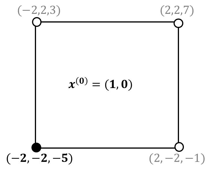
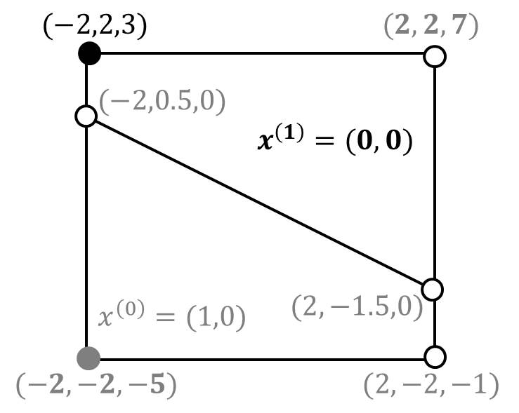
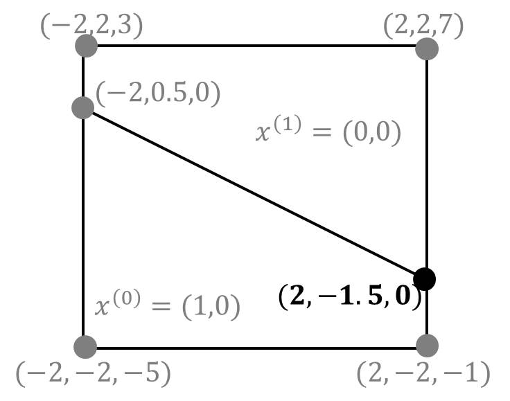
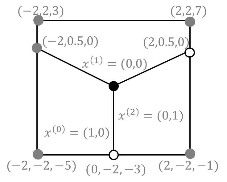
We explain the running process of DualSearch with a toy example. Let us consider an energy function $f(x_{1},x_{2})=x_{1}+x_{2}$, and two constraints $h_{1}$ and $h_{2}$ defined as follows.

$$h_{1}(x_{1},x_{2}) =x_{1}-x_{2},$$ (13)

$$h_{2}(x_{1},x_{2}) =2|x_{1}-x_{2}|.$$ (14)

Here, we set $M=2$. Initially, the algorithm computes a minimizer $x^{(0)}=(1,0)$ for $\lambda^{(0)}=(-2,-2)$. Then the initial ${\mathcal{V}}$ becomes $\{(-2,-2,-5),(-2,2,3),$ $(2,-2,-1),(2,2,7)\}$, which is shown in Figure 1. At this point, $X=\{x^{(0)}\}$. Let $(-2,2,3)\in{\mathcal{V}}$ be chosen in the next iteration, and for that vertex, the new minimizer $x^{(1)}\in\chi_{g}$ is found. This updates both $X=\{x^{(0)},x^{(1)}\}$ and the skeleton as shown in Figure 1. In the following iterations, $(2,2,7),(2,-2,-1)$ and $(-2,0.5,0)$ are chosen, but for those vertices, there is no new minimizer; that is, for those vertices, a minimizer is either $x^{(1)}=(1,0)$ or $x^{(2)}=(0,0)$. The skeleton at this point is shown in Figure 1. Next, $(2,-1.5,0)$ is chosen, and the new minimizer $x^{(2)}=(0,1)$ is computed so that $X$ is updated by $\{x^{(0)},x^{(1)},x^{(2)}\}$. This changes the skeleton as in Figure 1.

Figure 1: Skeletons projected onto two dimensional space. The black circle denotes the chosen vertex in that step. The gray circle denotes that the vertex is already processed and confirmed as a vertex of the final skeleton. The empty circle denotes a vertex not processed yet.

3.2 Correctness of the algorithm

In what follows, we analyze the correctness and query complexity of DualSearch. All proofs are provided in Section A.

Lemma 2.

At the end of each iteration of DualSearch, ${\mathcal{G}}={\mathcal{G}}_{g_{X}}$.

Lemma 2 states that when DualSearch terminates, ${\mathcal{G}}$ is the skeleton of an induced dual $g_{X}$ where $X$ is the output of the algorithm. It remains to show that the computed $X$ is indeed the characteristic set $\chi_{g}$.

Theorem 1.

When DualSearch terminates with $X$, $X=\chi_{g}$.

From Lemma 2 and Theorem 1, the following holds.

Corollary 1.

When DualSearch terminates, ${\mathcal{G}}={\mathcal{G}}_{\chi_{g}}$.

Now we analyze the query complexity. At each iteration, the algorithm uses exactly one oracle call. Then, either one new $v\in{\mathcal{V}}_{g}$ is identified if Line $5$ of Algorithm 1 is not satisfied, or one new $x\in\chi_{g}$ is obtained if Line $5$ is satisfied. Using these facts, we prove the following theorem.

Theorem 2.

The number of oracle calls in DualSearch is $|{\mathcal{V}}_{g}|+|\chi_{g}|$.

Recall that each $x\in\chi_{g}$ corresponds to a facet of the $(m+1)$-dimensional convex polytope of $g$. Since each vertex is determined as the intersection of at least $(m+1)$ facets, at the end of our algorithm, $|{\mathcal{V}}_{g}|$ is bounded by $O(|\chi_{g}|^{m+1})$. Thus, the query complexity becomes $O\left(poly(|\chi_{g}|)\right)$.

4 Algorithms for a specific constraint instance

In this section, we propose two variants of DualSearch to compute an approximate solution for a specific constraint instance. The first one is called DualMax, and the second one is AdaptSearch which combines DualMax and DualSearch. While DualSearch essentially does not need prior knowledge, DualMax and AdaptSearch explicitly use a given prior knowledge $\hat{b}$ for more efficient computation.

4.1 DualMax

Given $\hat{b}\in{\mathbb{R}}^{m}$, this algorithm finds the maximum of the dual $g$, which provides a lower bound of (3). If a corresponding minimizer of (3) is in $\chi_{g}$, this algorithm finds that minimizer efficiently. Even though the corresponding minimizer is not in $\chi_{g}$, the algorithm finds a lower bound of the minimum, which is a good approximate solution as shown in Section 5.1.2.

The main difference of DualMax from DualSearch is the vertex set appended to ${\mathcal{V}}$ in Line $7$ of Algorithm 1. At each iteration, DualMax calls the oracle for the maximum of the current induced dual. While DualSearch appends all vertices in ${\mathcal{V}}^{+}$, DualMax only appends one vertex $v\in{\mathcal{V}}^{+}$ where $z_{v}\geq z_{u}$ for all $u\in{\mathcal{V}}^{+}$. Then $z_{v}$ becomes the maximum of the induced dual for the next iteration. Since the (induced) dual is concave, such a local search on $S$ enables us to eventually find the maximum of the dual. The following is the modification of DualSearch to obtain DualMax.

1. The initial vertex set is changed to ${\mathcal{V}}^{\prime}=\{v\}$ where $z_{v}\geq z_{u}$ for all $u\in{\mathcal{V}}$ where ${\mathcal{V}}$ is the ordinary initial skeleton vertex.

2. Line 1 of Algorithm 1 is changed to “append to ${\mathcal{V}}$ the one vertex $v\in{\mathcal{V}}^{+}$ such that $z_{v}\geq z_{u}$ for all $u\in{\mathcal{V}}^{+}$”.

Then, the following Lemma holds, and the proof is provided in Appendix.

Lemma 3.

When DualMax terminates, for the last $v^{*}$ for which the oracle is called, $z_{v^{*}}=g(\lambda_{v^{*}})=\max_{\lambda}g(\lambda)$.

Note that DualMax uses far fewer oracle calls than DualSearch, which leads to fast computation of the maximum value of $g$ and the corresponding primal solution. The cutting plane method [6] can do the same computation as DualMax, and DualMax can be understood as one implementation of the cutting plane method. While the cutting plane method computes the maximum of the dual by linear programming with computed hyperplanes at each time, DualMax computes it by keeping and updating the skeleton of the dual.

Now, we suggest a way for DualMax to deal with inequality constraints by inserting a slack variable. For a given problem with inequality constraints, we first transform the problem to one with equality constraints, and apply the algorithm to the transformed problem. Let us consider the following problem.

$$\min_{x}\left\{f(x):\bar{b}-k\leq H(x)\leq\bar{b}\right\},$$ (15)

where $k\in{\mathbb{R}}^{m}$, and the inequality is the coordinatewise inequality. The inequality gap contains our prior knowledge, i.e. $\hat{b}_{i}\in[\bar{b}_{i}-k_{i},\bar{b}_{i}]$. First we transform the problem to a problem with equality constraints using a slack variable $y\in{\mathbb{R}}^{m}$ as follows.

$$\min_{x,y}\left\{\hat{f}(x,y):H(x)+y=\bar{b}\right\},$$ (16)

where $y\in\prod_{i=1}^{m}[0,k_{i}]$, and $\hat{f}(x,y)=f(x)$. Let us consider the following Lagrangian.

$$\hat{L}(x,y,\lambda)=\hat{f}(x,y)+\lambda^{T}(H(x)+y-\bar{b}).$$ (17)

For a minimizer $(x^{*},y^{*})$ of $\hat{L}$ for a fixed $\lambda$, it always holds that $y^{*}_{i}=0$ for $\lambda_{i}>0$, $y^{*}_{i}=k_{i}$ for $\lambda_{i}<0$, and $y^{*}$ can be any number in $[0,k_{i}]$ for $\lambda_{i}=0$. Hence, $y^{*}$ only depends on $\lambda$. Then, the dual $\hat{g}(\lambda)$ of $\hat{f}(x,y)$ becomes

$$\hat{g}(\lambda)=\min_{x}\left\{f(x)+\lambda^{T}(H(x)+y^{*}-\bar{b})\right\}.$$ (18)

Note that $\max_{\lambda}\hat{g}(\lambda)$ is a lower bound of (15). Since $y^{*}$ is determined only by $\lambda$, $\hat{g}(\lambda)$ can be computed by the same oracle for $g(\lambda)$. Now, we obtain the following lemma.

Lemma 4.

Let $(x^{*},y^{*})$ be such that $\hat{L}(x^{*},y^{*},\lambda^{*})=\hat{g}(\lambda^{*})$ for some $\lambda^{*}\in S$, and $b^{*}=H(x^{*})+y^{*}$. Then $f(x^{*})=\min_{x}\left\{f(x):b^{*}-k\leq H(x)\leq b^{*}\right\}$.

Proof.

Assume $(\hat{x},\hat{y})$ satisfying $H(\hat{x})+\hat{y}=b^{*}$. It implies that $\lambda^{T}(H(\hat{x})+\hat{y}-b^{*})=\lambda^{T}(H(x^{*})+y^{*}-b^{*})$ for any $\lambda\in{\mathbb{R}}^{m}$. Then, $\hat{g}(\lambda^{*})=\hat{L}(x^{*},y^{*},\lambda^{*})\leq L(\hat{x},\hat{y},\lambda^{*})$. Finally, $\hat{f}(x^{*},y^{*})\leq\hat{f}(\hat{x},\hat{y})$, and by the definition of $\hat{f}$, $f(x^{*})\leq f(\hat{x})$ holds. ∎

Hence, we can solve (15) by the same manner as in the equality case. Inequality constraints make DualMax more widely applicable because we may not know the exact statistics of a desired solution in practice.

4.2 AdaptSearch

DualSearch is a very effective algorithm because it finds minimizers for all $\lambda\in S$. But in general we do not know where good solutions are found, and thus we should use a large search region $S$, which leads to slow running time. On the other hand, while DualMax efficiently finds the maximum of the dual for a specific $\hat{b}$, it may be difficut to determine $\hat{b}$ for equality constraints in practice. Even if we use inequality constraints to deal with the uncertainty, as inequality gap gets larger, the accuracy of DualMax gets lower. To overcome these drawbacks, we propose a hybrid algorithm, called AdaptSearch, to combine advantages of DualMax and DualSearch, which runs as follows.

1. Let our prior knowledge $\hat{b}$ be given, and $S\subset{\mathbb{R}}^{m}$ be a large search region.

2. Run DualMax on $S$ with inequality constraint $\hat{b}-k^{-}\leq H(x)\leq\hat{b}+k^{+}$ for moderately small $k^{-},k^{+}>0$. Let $b^{*}$ be the constraint instance for which the dual maximum is computed.

3. Run DualMax again on $S$ with equality constraint $H(x)=b^{*}$. Then, we obtain $\lambda^{*}$ at which DualMax computes the maximum of the dual.

4. Run DualSearch for a small search region $\prod_{i=1}^{m}[\lambda^{*}_{i}-\alpha_{i},\lambda^{*}_{i}+\alpha_{i}]$ where $\alpha_{i}\geq 0$, and let $X^{*}$ be the output of DualSearch.

5. Output a solution among $X^{*}$ that minimizes the soft-constrained objective.

Note that in AdaptSearch, we can also use the cutting plane method instead of DualMax. In general, any convex search region is adoptable in Step $4$, but we observed from extensive experiments that small constants $\alpha_{i}$ are enough to obtain a good solution. We will show in Section 5 that AdaptSearch computes better solutions than DualMax and runs quite fast.

5 Applications

5.1 Labelling problems in computer vision

In computer vision, a number of problems can be reduced to labelling problems, including image segmentation, $3$D-reconstruction, and stereo. Our constrained energy minimization algorithms can be applied to those problems, for instance, when we may have knowledge on the volume of a reconstructed object for $3$D-reconstruction or on the number of pixels belonging to an object for image segmentation. In this section, we show how our algorithms are applied to the foreground-background (fg-bg) image segmentation problem.

The fg-bg image segmentation problem is to divide a given image to foreground (object) and background. This can be done by labelling all pixels such that $1$ is assigned to foreground pixels and $0$ is assigned to background pixels. For this problem, one popular approach is to consider an image as a grid graph in which each node has four neighbours, and minimize an energy function $f$ of the form (2), which is submodular. The unary terms of the function encode how likely each pixel belongs to the foreground or background, while the pairwise terms encode the smoothness of the boundary of the object being segmented. However, in general, a minimizer of (2) is not the ground truth, and it has been shown that imposing statistics on a desired solution can improve segmentation results [12].

Below, we describe some linear constraints that have been successfully used in computer vision.

1. Size: $\sum_{i\in V}x_{i}=b$ where $b\in{\mathbb{R}}$ [20, 35, 36].

2. Mean: $\sum_{i\in V}\frac{c_{i}x_{i}}{\sum_{i\in V}x_{i}}=b$ where $b\in{\mathbb{R}}^{2}$ and $c_{i}=(v_{i},h_{i})\in{\mathbb{R}}^{2}$ denotes the vertical and horizontal coordinates of a pixel $i$, respectively [12].

3. Cov.: $\sum_{i\in V}\frac{(v_{i}-\mu_{v})(h_{i}-\mu_{h})x_{i}}{\sum_{i\in V}x_{i}}=b$ where $b\in{\mathbb{R}}$ and $(\mu_{v},\mu_{h})\in{\mathbb{R}}^{2}$ denotes the mean center of the object [12].

We can define the variance constraints for the vertical and horizontal coordinates in a similar way to the covariance constraint.

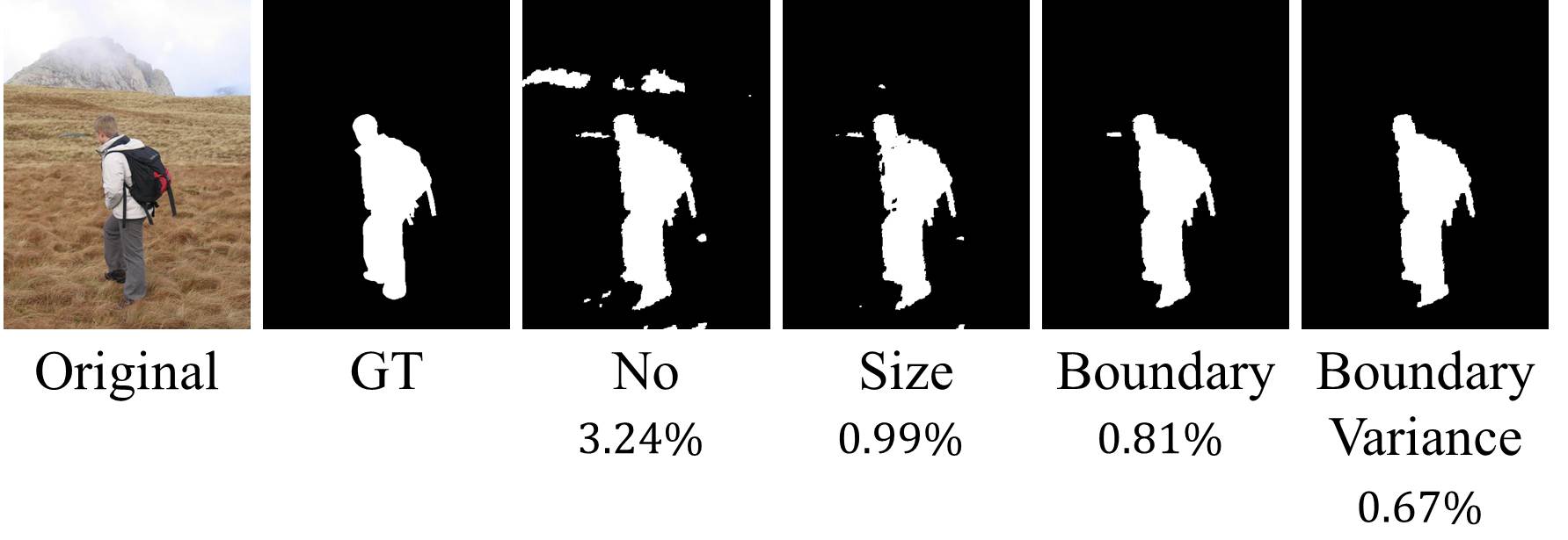
In many scenarios, researchers are interested in ensuring that the boundary of the object in the segmentation has a particular length. This length can be measured by counting the number of pairs of adjacent variables having different labels and described by $\sum_{(i,j)\in E}|x_{i}-x_{j}|=b$ where $b\in{\mathbb{R}}$. For this boundary constraint, the search region $S$ may be restricted to a subregion of ${\mathbb{R}}\times[K,\infty]$ where $K\leq 0$ is the smallest real number ensuring $L(x,\lambda)$ submodular for all $\lambda\in S$. Figure 2 shows improvement of segmentation results by imposing the above constraints.

Figure 2: The segmentation labelled by No is obtained by minimizing the energy function with no constraint. The last three segmentations were obtained by DualMax with the specified constraints whose instances are set by the ground truth statistics. For each segmentation, the pixel-by-pixel error with respect to the ground truth is reported.

5.1.1 Query complexity of DualSearch

Recall that the query complexity of DualSearch is polynomial in $|\chi_{g}|$. Note that $|\chi_{g}|$ is upper bounded by the number $C$ of all possible constraint instances. For all the constraints above, we can show $C=O(poly(n))$. For example, for the size constraint, $C=n$, and for the boundary length constraint, $C\leq 2n$ because $G$ is a grid graph. Let us consider the mean constraint, and let $\hat{b}\in{\mathbb{R}}^{2}$ be obtained from our prior knowledge. Then, the Lagrangian is as follows:

$$L(x,\lambda)=f(x)+\lambda^{T}\left(\sum_{i}(c_{i}-\hat{b})x_{i}\right),$$ (19)

where $c_{i}\in{\mathbb{Z}}^{2}$ is bounded by the size of row and column of the image. Hence, the numbers of possible values of $\sum_{i}c_{i}x_{i}$ and $\hat{b}\sum_{i}x_{i}$ are $O(n^{2})$ and $O(n)$, respectively, which leads to $C=O(n^{3})$. By a similar analysis, we can show $C=O(n^{3})$ for the covariance and variance constraints. If we consider multiple constraints simultaneously, $C$ is bounded by multiplication of the upper bound of each constraint. Hence, $|\chi_{g}|=O(poly(n))$ for any combination of the constraints above.

5.1.2 Experiments

First we did experiments for the size and boundary constraints, and used the following Lagrangian.

$$L(x,\lambda)=f(x)+\\ \lambda_{1}\sum_{i\in V}x_{i}+\lambda_{2}\sum_{(i,j)\in E}|x_{i}-x_{j}|.$$ (20)

Table 1: Results of DualSearch on $12$ images from [27] each of which has the size $120\times 120$.

	$|{\mathcal{V}}_{g}|$	$|\chi_{g}|$	Time		$|{\mathcal{V}}_{g}|$	$|\chi_{g}|$	Time
IM1	273K	286K	25m	IM5	306K	325K	31m
IM2	168K	170K	16m	IM6	238K	252K	27m
IM3	105K	107K	14m	IM7	248K	248K	23m
IM4	114K	127K	15m	IM8	300K	308K	31m

Table 1 reports the summary of results of DualSearch for $12$ images with size $120\times 120$. DualSearch produces minimizers for a very large number of constraint instances. One implication is that for any given constraint instance, DualMax and AdaptSearch can compute a minimizer with very close constraint instance to the original one. Figure3 shows an example of a skeleton projected onto two dimensional $\lambda$ space that is computed with (20) for a $12\times 12$ image.

Figure 3: Example of a skeleton projected onto two dimensional space, computed with (20).

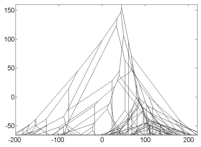
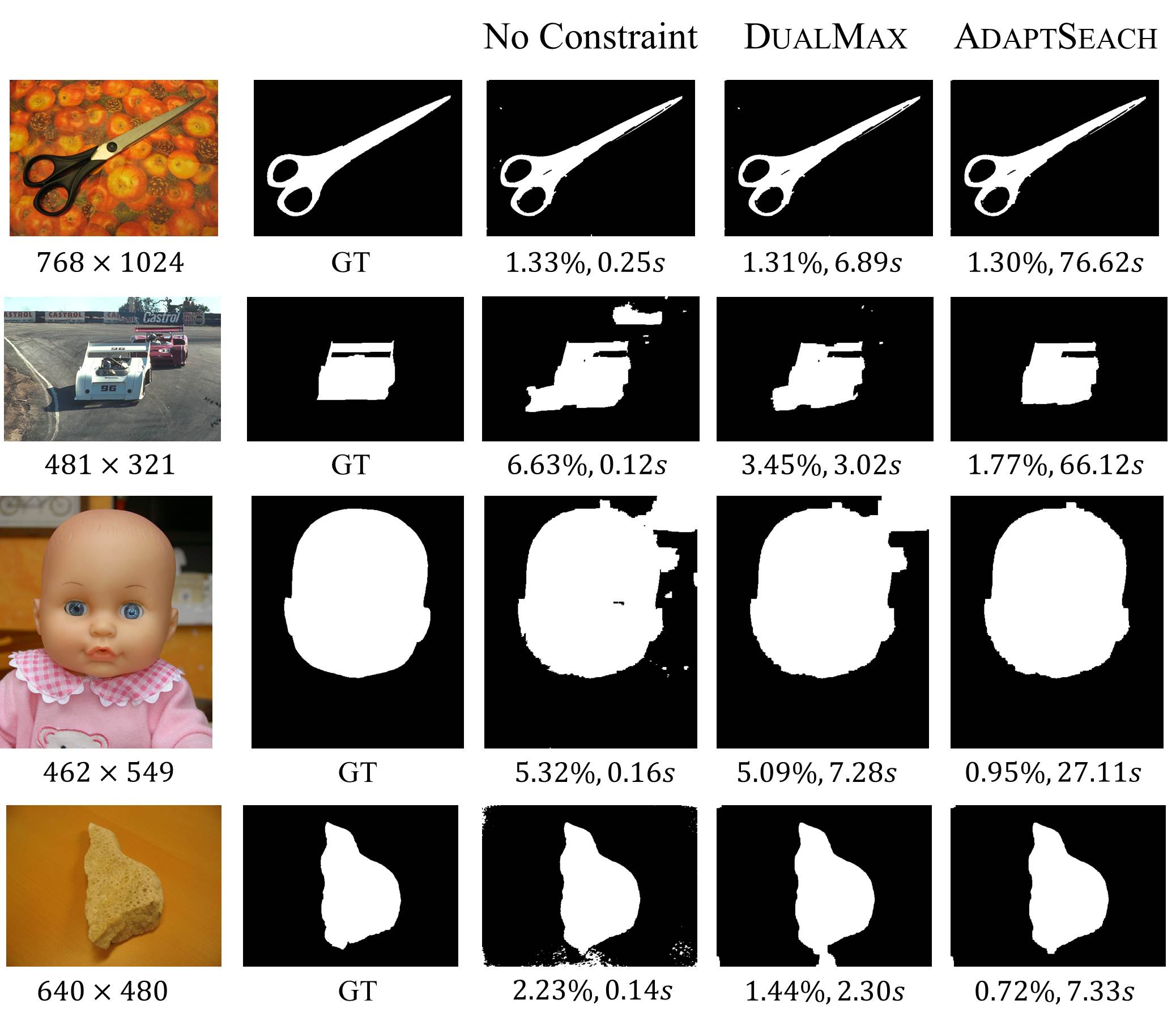
Figure 4 shows experimental results of DualMax and AdaptSearch. For AdaptSearch, we used a soft constraint with a square penalty function for the size and the boundary length constraint, that is, $\eta_{1}(\sum_{i}x_{i}-\hat{b}_{1})^{2}$ and $\eta_{2}(\sum_{(i,j)\in E}|x_{i}-x_{j}|-\hat{b}_{2})^{2}$. We chose $\eta_{1}=1$ and $\eta_{2}=100$ with which segmentation results generally show less error. Also for the first running of DualMax, we used the inequality gap $k^{+},k^{-}$ of $\pm 10\%$ of $\hat{b}$, and $\hat{b}_{1},\hat{b}_{2}$ were obtained from the ground truth. The small search region to apply DualSearch is used with $\alpha_{1}=\alpha_{2}=1$, except for the first image with $\alpha_{1}=\alpha_{2}=0.3$.

Figure 4: Segmentation results by minimizing (2), DualMax and AdaptSearch each of which is labelled by the pixel-by-pixel error with respect to the ground truth and its running time. The used images are from [28].

We also compared our algorithms with LP [18] and QP [12] relaxation based methods. Table 2 shows that DualMax is faster and more accurate compared with both methods. Since LP and QP cannot handle higher order both-side constrained inequality constraints unlike our algorithms, we used linear constraints introduced previously. Segmentation results are provided in Appendix.

Table 2: Comparison of DualMax and two continuous relaxation based methods with inequality gap $\pm 5\%$. The values are averaged over 6 images from [28] of size $321\times 481$.

Const.	DualMax		LP		QP
	Err.	Time	Err.	Time	Err.	Time
Sz,Mn	3.37	1.73	3.46	83.6	3.95	349
Sz,Vr	2.34	1.91	2.73	77.2	2.64	461

Err.: pixel-by-pixel error with respect to the ground truth $(\%)$.
Time: in seconds.   Const.: constraints.
Sz: size, Mn: Mean, Vr: variance.

5.2 Combinatorial optimization

Submodular minimization

Our method can also be used for constrained submodular function minimization (SFM). SFM is known to be polynomial time solvable and a number of studies have considered SFM under specific constraints such as vertex cover and size constraints [10, 22]. In contrast to previous work, we provide a framework for dealing with multiple general constraints. Our method can not only deal with any linear constraint, but can also handle some higher order constraints which ensure that the dual is computable. For instance, as shown in the previous section, any submodular constraint $h_{i}(x)$ can be handled with restricted $\lambda_{i}\geq 0$.

Shortest path problem

The restricted shortest path problem is a widely studied constrained version in which each edge has an associated delay in addition to its length. A path is feasible if its total delay is less than some threshold $D$ [21]. This is a linear constraint $\sum_{i}d_{i}x_{i}\leq D$ where $d_{i}$ is the delay of edge $i$. Another natural constraint for the shortest path problem is to drop some $k$ nodes among a given set of $m$ nodes. For instance, we may want to design a tour that should contain $k$ cities among $m$ cities. Indeed, this becomes a Hamiltonian path problem when $k=m=n$. As in the project selection problem, we may partition $n$ cities to $r$ groups, and try to visit $k_{i}$ number of cities from each group where $1\leq i\leq r$. Note that all constraints above are linear so that our method can be applied.

Project selection problem

Given a set $P$ of projects, a profit function $q:P\rightarrow{\mathbb{R}}$, and a prerequisite relation $R\subseteq P\times P$, this problem is to find projects maximizing the total profit while satisfying a prerequisite relation. This is also known as the maximal closure problem and can be solved in polynomial time by transforming it to a st-mincut problem [25]. In practice, $P$ may be represented by sets $P_{1},\ldots,P_{m}$ that may overlap, and we may want to select $k_{i}$ projects from $P_{i}$ for $1\leq i\leq m$. This can be formulated using linear constraints $k_{i}=u_{i}^{T}x$ where $u_{i}$ is an indicator which projects belong to $P_{i}$. This enables the use of our method to solve the constrained project selection problem.

6 Conclusions

This paper proposes novel algorithms to deal with the multiple constrained MAP inference problem. Our algorithm AdaptSearch is able to generate high-quality candidate solutions in a short time (see Figure 4) and enables handling of problems with very high order potential functions. We believe it would have a significant impact on the solution of many labelling problems encountered in computer vision and machine learning. As future work, we intend to analyze the use of our algorithms for enforcing statistics in problems encountered in various domains of machine learning.

Appendix

A Proofs

In this section, we provide the proofs omitted in the main body. We use notations ${\mathcal{G}}(t),$ ${\mathcal{V}}^{+}(t),$ ${\mathcal{V}}^{-}(t)$ and $X(t)$ to indicate ${\mathcal{V}}^{+},{\mathcal{V}}^{-},{\mathcal{G}}$ and $X$ at the end of the $t$-th iteration in lgorithm 1, respectively. Also we denote a vertex chosen in Line $3$ at the $t$-th iteration by $v$, and $\Gamma_{X}(S)$ by $\Gamma_{X}$ without $S$. Note that initially ${\mathcal{G}}(0)={\mathcal{G}}_{g_{X}}$ by the definition of $InitSkeleton()$.

A.1 Proof of Lemma 2

Lemma 2 is proved by the following Lemma 5 and Lemma 6.

Lemma 5.

Assume that ${\mathcal{G}}(t-1)={\mathcal{G}}_{g_{X(t-1)}}$. Then ${\mathcal{V}}(t)={\mathcal{V}}_{g_{X(t)}}$.

Proof.

$(\Longrightarrow)$ Let $u\in{\mathcal{V}}(t)$. First assume that $u$ is also in ${\mathcal{V}}(t-1)$. Suppose that $u\notin{\mathcal{V}}_{g_{X(t)}}$. There is $Q\subseteq\Gamma_{X(t)}$ and $Q\cap\{u\}=\emptyset$ so that $u$ is a proper convex combination of $Q$. Note that $\Gamma_{X(t)}\subseteq\Gamma_{X(t-1)}$. Thus, $u$ is a proper convex combination of $Q$ over $\Gamma_{X(t-1)}$. It is a contradiction to $u\in{\mathcal{V}}(t-1)$.

Assume that $u\notin{\mathcal{V}}(t-1)$. Then, $u\in{\mathcal{V}}^{+}(t)$, implying that $u\in e(u_{1},u_{2})\in{\mathcal{E}}(t-1)$ and $u\in P_{x_{v}}$. Suppose that there is $Q\subseteq\Gamma_{X(t)}$ and $Q\cap\{u\}=\emptyset$ so that $u$ is a proper convex combination of $Q$. Since $Q\nsubseteq e(u_{1},u_{2})$ and $\Gamma_{X(t)}\subseteq\Gamma_{X(t-1)}$, it is a contradiction to the definition of ${\mathcal{E}}(t-1)$.

$(\Longleftarrow)$ Let $u\in{\mathcal{V}}_{g_{X(t)}}$. Suppose that $u\notin{\mathcal{V}}(t)$ but $u\in{\mathcal{V}}(t-1)$, which means that $u\in{\mathcal{V}}^{-}$. Then, $z_{u}>g_{X(t)}(\lambda_{u})$, a contradiction to $u\in{\mathcal{V}}_{g_{X(t)}}$. Suppose that $u\notin{\mathcal{V}}(t)$ nor $u\notin{\mathcal{V}}(t-1)$. Then, there is $Q\subset\Gamma_{X(t-1)}$ and $Q\cap\{u\}=\emptyset$ so that $u$ is a proper convex combination of $Q$. Note that $Q\nsubseteq P_{x_{v}}$ because $u\in{\mathcal{V}}_{g_{X(t)}}$. Since $z_{u}\leq P_{x_{v}}(\lambda_{u})$, at least one of $Q$ is strictly below $P_{x_{v}}$, and let $Q^{-}$ be the set of such elements of $Q$. Since $u\in{\mathcal{V}}_{g_{X(t)}}$, at least one of $Q$ is strictly above $P_{x_{v}}$, and let $Q^{+}$ be the set of such elements of $Q$. Let $P$ be the set of intersections of $e(q^{-},q^{+})$ and $P_{x_{v}}$ where $q^{-}\in Q^{-}$ and $q^{+}\in Q^{+}$. Suppose that $u$ is strictly below $P_{x_{v}}$, then $u$ is a proper convex combination of $P$ and $Q^{-}\subset\Gamma_{X(t)}$, implying a contradiction. So $u\in P_{x_{v}}$. Suppose that $|P|>1$, then $u$ is a proper convex combination of $P\subset\Gamma_{X(t)}$, which is a contradiction. Thus, $|P|=1$ and $u\in P_{x_{v}}$. Then since $u$ is on some edge $e(w_{1},w_{2})\in{\mathcal{E}}(t-1)$ and $u\in P_{x_{v}}$, $u\in{\mathcal{V}}^{+}(t)$ by the algorithm so that $u$ is present in ${\mathcal{V}}(t)$, which is a contradiction. ∎

Lemma 6.

Assume that ${\mathcal{G}}(t-1)={\mathcal{G}}_{g_{X(t-1)}}$. Then ${\mathcal{E}}(t)={\mathcal{E}}_{g_{X(t)}}$.

Proof.

$(\Longrightarrow)$ Let $e(u,w)\in{\mathcal{E}}(t)$. Assume that $e(u,w)$ is added by ${\mathcal{E}}^{+}$ so that $w$ is the intersection of $e(u,u^{\prime})\in{\mathcal{E}}(t-1)$ and $P_{x_{v}}$. Suppose that there is $Q\subset\Gamma_{X}(t)$, and $Q\nsubseteq e(u,w)$ so that for some $p\in e(u,w)$, $p$ is a proper convex combination of $Q$. Since $\Gamma_{X(t)}\subseteq\Gamma_{X(t-1)}$, $Q\subseteq\Gamma_{X(t-1)}$. Also since $Q\subset\Gamma_{X(t)}$ and $Q\nsubseteq e(u,w)$, $Q\nsubseteq e(u,u^{\prime})$. It is a contradiction to $p\in e(u,u^{\prime})\in{\mathcal{E}}(t-1)$.

Assume that $e(u,w)\in{\mathcal{E}}(t-1)$. Since $\Gamma_{X(t)}\subseteq\Gamma_{X(t-1)}$, no $p\in e(u,w)$ is a proper convex combination of $Q\in\Gamma_{X(t)}$ and $Q\nsubseteq e(u,w)$. Thus, $e(u,w)\in{\mathcal{E}}_{g_{X(t)}}$ due to $u,w\in{\mathcal{V}}(t)={\mathcal{V}}_{g_{X(t)}}$ by Lemma 5.

Assume that $e(u,w)$ is added by $ConvEdge({\mathcal{V}}^{+}(t))$. Suppose that there is $Q\subset\Gamma_{X(t)}$ and $Q\nsubseteq e(u,w)$ so that for some $p\in e(u,w)$, $p$ is a proper convex combination of $Q$. Since $p\in e(u,w)\in ConvEdge({\mathcal{V}}^{+}(t))\subset P_{x_{v}}$, $Q\subset\Gamma_{X(t)}\cap P_{x_{v}}$. Since $e(u,w)$ is an edge of the convex hull of ${\mathcal{V}}^{+}(t)$, any $p\in e(u,w)$ cannot be a proper convex combination of $Q$, which is a contradiction.

$(\Longleftarrow)$ Let $e(u,w)\in{\mathcal{E}}_{g_{X(t)}}$. Suppose that $e(u,w)\notin{\mathcal{E}}(t)$. If $u\in{\mathcal{V}}^{-}$ or $w\in{\mathcal{V}}^{-}$, it is a contradiction to $e(u,w)\in{\mathcal{E}}_{g_{X(t)}}\subset 2^{\Gamma_{X(t)}}$. If both $u,w\in{\mathcal{V}}^{+}(t)$, by the definition of $ConvEdge({\mathcal{V}}^{+})$, and the fact that $e(u,w)\notin{\mathcal{E}}(t)$, $e(u,w)\notin{\mathcal{E}}_{g_{X(t)}}$, which is a contradiction. Therefore one of $u,w$ belongs to ${\mathcal{V}}(t-1)\cap{\mathcal{V}}(t)$, and the other belongs to ${\mathcal{V}}^{+}(t)$. Without loss of generality, let $u\in{\mathcal{V}}(t-1)\cap{\mathcal{V}}(t)$ and $w\in{\mathcal{V}}^{+}(t)$, then $u$ must be strictly below $P_{x_{v}}$. Then, $e(u,w)\notin{\mathcal{E}}(t-1)$. There is $Q\in\Gamma_{X(t-1)}$ so that $Q\nsubseteq e(u,w)$ and for some $p\in e(u,w)$, $p$ is a proper convex combination of $Q$. If all $q\in Q$ are strictly above $P_{x_{v}}$, $p$ is also strictly above $P_{x_{v}}$. If for all $q\in Q$, $z_{q}\leq P_{x_{v}}(\lambda_{q})$, $Q\subset\Gamma_{X(t)}$, implying a contradiction to $e(u,w)\in{\mathcal{E}}_{g_{X(t)}}$. Thus, at least one of $Q$ is strictly below $P_{x_{v}}$, and let $Q^{-}$ be the set of such elements of $Q$. Also at least one of $Q$ is strictly above $P_{x_{v}}$, and let $Q^{+}$ be the set of such elements of $Q$. Let $P$ be the set of intersections of $e(q^{-},q^{+})$ and $P_{x_{v}}$ where $q^{-}\in Q^{-}$ and $q^{+}\in Q^{+}$. If $|P|>1$ or $p\notin P$, $p$ is a proper convex combination of $Q^{-}$ and $P$. Thus, $|Q^{-}|=|Q^{+}|=1$ and $p\in P_{x_{v}}$. This holds for all $p\in e(u,w)$, which means that $e(u,w)\in P_{x_{v}}$. This is a contradiction to the fact that $u$ is strictly below $P_{x_{v}}$. ∎

A.2 Proof of Theorem 1

Proof.

Let ${\mathcal{G}}=({\mathcal{V}},{\mathcal{E}})$ be the skeleton at the end of DualSearch. It holds that $X\subseteq\chi_{g}$ for each iteration by the algorithm. Suppose that there is $x^{*}\in\chi_{g}\backslash X$ when the algorithm terminates. Then, there is $\lambda^{*}\in S$ such that $P_{x^{*}}(\lambda^{*})<P_{x}(\lambda^{*})$ for every $x\in X$. Also there is $\hat{x}\in X$ such that $P_{\hat{x}}(\lambda^{*})=g_{X}(\lambda^{*})$. Then, $(\lambda^{*},P_{\hat{x}}(\lambda^{*}))$ can be represented as a convex combination of ${\mathcal{V}}^{\prime}\subset{\mathcal{V}}$ such that $P_{\hat{x}}(\lambda_{v})=g_{X}(\lambda_{v})$ for all $v\in{\mathcal{V}}^{\prime}$. By a property of the algorithm, $P_{x^{*}}(\lambda_{v})\geq P_{\hat{x}}(\lambda_{v})=g_{X}(\lambda_{v})=g(\lambda_{v})$ for each $v\in{\mathcal{V}}^{\prime}$. Since $\lambda^{*}$ is a convex combination of $\{\lambda_{v}:v\in{\mathcal{V}}^{\prime}\}$, we have $P_{x^{*}}(\lambda^{*})\geq P_{\hat{x}}(\lambda^{*})$. This implies a contradiction to $P_{x^{*}}(\lambda^{*})<P_{\hat{x}}(\lambda^{*})$. ∎

A.3 Proof of Theorem 2

Proof.

For each iteration, there is exactly one oracle call. Let $C$ be a set of confirmed vertices $u$, that is, $z_{u}=g(\lambda_{u})$. Note that at each iteration, either $|C|$ or $|X|$ increases by one, depending on whether $P_{x_{v}}(\lambda_{v})<z_{v}$, and confirmed vertices are never removed from ${\mathcal{V}}$. When the algorithm terminates, $|X|=|\chi_{g}|$ by Theorem 1 and $|C|=|{\mathcal{V}}_{g}|$ by Corollary 1. Thus, the algorithm uses $|{\mathcal{V}}_{g}|+|\chi_{g}|$ number of oracle calls. ∎

A.4 Proof of Lemma 3

Proof.

First we prove that for every iteration, a chosen $v$ satisfies that $z_{v}=\max_{\lambda}g_{X}(\lambda)$. It initially holds by the definition of $v$. Assume that at the $(t-1)$-th iteration, the statement holds. Let $v$ be chosen in the $t$-th iteration. If $P_{x_{v}}(\lambda_{v})\geq z_{v}$, there is no change on $X$ and ${\mathcal{G}}$ so that the statement holds, and the algorithm terminates. When $P_{x_{v}}(\lambda_{v})<z_{v}$, let $\hat{v}\in{\mathcal{V}}^{+}$ be such that $z_{\hat{v}}\geq z_{u}$ for all $u\in{\mathcal{V}}^{+}$. Suppose that there is $\bar{v}\in{\mathcal{V}}(t)$ such that $z_{\bar{v}}>z_{\hat{v}}$ and $z_{\bar{v}}$ is the maximum value of $g_{X(t)}$. Note that $z_{v}$ is the maximum value of $g_{X(t-1)}$ by the assumption. Suppose $z_{\bar{v}}=z_{v}$, and let $P\subseteq{\mathcal{V}}(t-1)$ be the set such that for every $p\in P$, $z_{p}=z_{v}$. Since $\bar{v}\in{\mathcal{V}}(t)$, $z_{\bar{v}}\leq P_{x_{v}}(\lambda_{\bar{v}})$ and $z_{v}>P_{x_{v}}(\lambda_{v})$. Then, some edge between two vertices of $P$ should intersect with $P_{x_{v}}$ due to the concavity of $g_{X(t)}$, and let $v^{\prime}$ be the intersection. Then, $z_{v}=z_{v^{\prime}}=z_{\hat{v}}$, which is a contradiction to $z_{\bar{v}}>z_{\hat{v}}$.

In ${\mathcal{G}}_{X(t-1)}$, since $\bar{v}$ is not the maximum, and by the concavity of $g_{X(t-1)}$, there is at least one edge $e(\bar{v},\bar{v}^{\prime})$ where $\bar{v}^{\prime}\in{\mathcal{V}}(t-1)$ such that $z_{\bar{v}^{\prime}}>z_{\bar{v}}$. In order that $z_{\bar{v}}$ becomes the maximum of $g_{X(t)}$, $\bar{v}^{\prime}$ should not belong to ${\mathcal{V}}(t)$, implying that $z_{\bar{v}^{\prime}}>P_{x_{v}}(\lambda_{\bar{v}^{\prime}})$. Then, there is intersection $q$ of $P_{x_{v}}$ and $e(\bar{v},\bar{v}^{\prime})$, implying that $z_{q}\geq z_{\bar{v}}$. If $z_{q}>z_{\bar{v}}$, it is a contradiction to the fact that $z_{\bar{v}}$ is the maximum value of $g_{X(t)}$ due to $q\in{\mathcal{V}}(t)$. If $z_{q}=z_{\bar{v}}$, it means that $z_{\bar{v}}\in{\mathcal{V}}^{+}$ and thus $z_{\bar{v}}=z_{\hat{v}}$, which is a contradiction to $z_{\bar{v}}>z_{\hat{v}}$.

We have proved that when the algorithm terminates, $z_{v}=\max_{\lambda}g_{X}(\lambda)\geq\max_{\lambda}g(\lambda)$. Let the last $v$ be $v^{*}$. In the last iteration, $z_{v^{*}}=P_{x_{v^{*}}}(\lambda^{*})=g(\lambda^{*})\leq\max_{\lambda}g(\lambda)$. ∎

B Segmentation results for Table 2

References

- [1] Barber, C.B., Dobkin, D.P., Huhdanpaa, H.: The quickhull algorithm for convex hulls. ACM Transactions on Mathematical Software (TOMS) 22 (1996)
- [2] Boros, E., Hammer, P.: Pseudo-boolean optimization. Discrete Applied Mathematics (2002)
- [3] Boykov, Y., Veksler, O., Zabih, R.: Fast approximate energy minimization via graph cuts. PAMI (2001)
- [4] Carreira, J., Sminchisescu, C.: CPMC: Automatic object segmentation using constrained parametric min-cuts. IEEE Trans. Pattern Anal. Mach. Intell. 34, 1312–1328 (2012)
- [5] Gallo, G., Grigoriadis, M., Tarjan, R.: A fast parametric maximum flow algorithm and applications. SIAM J. on Comput. 18, 18:30–55 (1989)
- [6] Guignard, M.: Lagrangean relaxation. TOP 11 (2003)
- [7] Gupta, R., Diwan, A.A., Sarawagi, S.: Efficient inference with cardinality-based clique potentials. In: Z. Ghahramani (ed.) ICML, ACM International Conference Proceeding Series, vol. 227, pp. 329–336. ACM (2007)
- [8] Hastings, M.B.: Community detection as an inference problem. Phys. Rev. E 74, 035,102 (2006). DOI 10.1103/PhysRevE.74.035102
- [9] Ishikawa, H.: Transformation of general binary MRF minimization to the first-order case. PAMI 33, 1234–1249 (2011)
- [10] Iwata, S., Nagano, K.: Submodular function minimization under covering constraints. In: FOCS (2009)
- [11] Kindermann, R., Snell, J.L.: Markov Random Fields and Their Applications. AMS (1980)
- [12] Klodt, A., Cremers, D.: A convex framework for image segmentation with moment constraints. In: ICCV (2011)
- [13] Kolev, K., Cremers, D.: Integration of multiview stereo and silhouettes via convex functionals on convex domains. In: ECCV (2008)
- [14] Kolmogorov, V., Boykov, Y., Rother, C.: Application of parametric maxflow in computer vision. In: ICCV (2007)
- [15] Kolmogorov, V., Rother, C.: Minimizing non-submodular functions with graph cuts - a review. In: PAMI (2007)
- [16] Komodakis, N., Paragios, N., Tziritas, G.: MRF optimization via dual decomposition: message-passing revisited. In: ICCV (2007)
- [17] Ladicky, L., Russell, C., Kohli, P., Torr, P.: Graph cut based inference with co-occurrence statistics. In: ECCV (2010)
- [18] Lempitsky, V., Kohli, P., Rother, C., Sharp, T.: Image segmentation with a bounding box prior. In: ICCV (2009)
- [19] Li, S.Z.: Markov random filed models in computer vision. In: ECCV (1994)
- [20] Lim, Y., Jung, K., Kohli, P.: Energy minimization under constraints on label counts. In: ECCV (2010)
- [21] Lorenz, D.H., Raz, D.: A simple efficient approximation scheme for the restricted shortest path problem. Operations Research Letters 28, 213–219 (1999)
- [22] Nagano, K., Kawahara, Y., Aihara, K.: Size-constrained submodular minimization through minimum norm base. In: ICML (2011)
- [23] Naor, J., Schwartz, R.: Balanced metric labeling. In: STOC (2005)
- [24] Nowozin, S., Lampert, C.: Global connectivity potentials for random field models. In: CVPR (2009)
- [25] Picard, J.C.: Maximal closure of a graph and applications to combinatorial problems. Management Science 22 (1976)
- [26] Ramalingam, S., Kohli, P., Alahari, K., Torr, P.: Exact inference in multi-label CRFs with higher order cliques. In: CVPR (2008)
- [27] Rhemann, C., Rother, C., Rav-Acha, A., Sharp, T.: High resolution matting via interactive trimap segmentation. In: CVPR (2008)
- [28] Rother, C., Kolmogorov, V., Blake, A.: “grabcut”: interactive foreground extraction using iterated graph cuts. ACM Trans. Graph. (2004)
- [29] Sinha, S., Pollefeys, M.: Multi-view reconstruction using photo-consistency and exact silhouette constraints: A maximum-flow formulation. In: ICCV (2005)
- [30] Strandmark, P., Kahl, F.: Parallel and distributed graph cuts by dual decomposition. In: CVPR (2010)
- [31] Toyoda, T., Hasegawa, O.: Random field model for integration of local information and global information. PAMI 30, 1483–1489 (2008)
- [32] Vicente, S., Kolmogorov, V., Rother, C.: Graph cut based image segmentation with connectivity priors. In: CVPR (2008)
- [33] Wainwright, M., Jaakkola, T., Willsky, A.: MAP estimation via agreement on trees: message-passing and linear programming. IEEE Transactions on Information Theory (2005)
- [34] Weiss, Y., Yanover, C., Meltzer, T.: MAP estimation, linear programming and belief propagation with convex free energies. In: UAI (2007)
- [35] Werner, T.: High-arity interactions, polyhedral relaxations, and cutting plane algorithm for soft constraint optimisation (MAP-MRF). In: CVPR (2008)
- [36] Woodford, O., Rother, C., Kolmogorov, V.: A global perspective on MAP inference for low-level vision. In: ICCV (2009)
- [37] Woodford, O.J., Rother, C., Kolmogorov, V.: A global perspective on map inference for low-level vision. In: ICCV, pp. 2319–2326. IEEE (2009)
- [38] Yanover, C., Meltzer, T., Weiss, Y.: Linear programming relaxations and belief propagation – an empirical study. Journal of Machine Learning Research 7, 1887–1907 (2006)