Non-Markovian Dynamical Maps:
Numerical Processing of Open Quantum Trajectories

Abstract

The initial stages of the evolution of an open quantum system encode the key information of its underlying dynamical correlations, which in turn can predict the trajectory at later stages. We propose a general approach based on non-Markovian dynamical maps to extract this information from the initial trajectories and compress it into non-Markovian transfer tensors. Assuming time-translational invariance, the tensors can be used to accurately and efficiently propagate the state of the system to arbitrarily long time scales. The non-Markovian transfer tensor method (TTM) demonstrates the coherent-to-incoherent transition as a function of the strength of quantum dissipation and predicts the non-canonical equilibrium distribution due to the system-bath entanglement. TTM is equivalent to solving the Nakajima-Zwanzig equation, and therefore can be used to reconstruct the dynamical operators (the system Hamiltonian and memory kernel) from quantum trajectories obtained in simulations or experiments. The concept underlying the approach can be generalized to physical observables with the goal of learning and manipulating the trajectories of an open quantum system.

Introduction.—The dynamics of large open quantum systems are of interest to a broad range of disciplines, including condensed matter physics, ultrafast spectroscopy, and quantum information technology, just to name a few. Of particular interest is the interaction between the system under study and the environment to which it couples. Within the fast bath approximation, the evolution of the system’s density matrix is dictated by a Lindbladian superoperator and can be regarded as a linear Markovian process. Nevertheless, in general the quantum trajectory of the open system is entangled with the bath and is therefore temporally correlated, i.e., non-Markovian. The analysis and simulation of this correlation is a daunting task, which often requires resources that scale exponentially with the system size. The root of the problem is the lack of a compact but complete representation of the information encoded in open quantum trajectories. The standard approaches fall into two classes: quantum master equations and path integral simulations. The first class of approaches is based on formally exact equations of motion, such as the Nakajima-Zwanzig formalism Breuer and Petruccione (2007); Nakajima (1958); Zwanzig (1960) or others, but restricted to either weak damping, high-temperature, short memory time or short simulation time Ishizaki and Tanimura (2005); Cao (1997); Koch et al. (2003); Hughes et al. (2009); Gualdi and Koch (2013); Breuer (2004); Piilo et al. (2008). The second class of approaches adopts the harmonic bath assumption which renders the use of stochastic Gaussian sampling or influence functional possible Egger et al. (2000); Makri and Makarov (1995), but does not converge well with the system size, the length of the memory time or the strength of the dissipation. To overcome these difficulties, we need a radically different approach to dissipative quantum dynamics.

In this letter, we propose a unified method to characterize, reconstruct, and propagate quantum trajectories which are non-locally correlated in time. It applies to any form of the system-bath Hamiltonian and scales favorably with respect to the system size and length of the time correlation. The scheme is based on a black-box analysis that extracts all available information from samples of initial trajectories generated experimentally or numerically. This information is stored in a collection of non-Markovian dynamical maps, which describes the propagation of the initial state of the system to a later time with full account for the time correlations in the trajectories. Then, a transformation of these maps is performed to obtain a set of transfer tensors that sort out correlations over different times. These tensors are the central object of this letter and serve two purposes: On the one hand, under the assumption of time-translational invariance, the tensor formalism can be used in a multiplicative fashion to propagate the state of the system to arbitrarily long times, leading to a non-perturbative and efficient algorithm for simulating dissipative quantum systems. On the other hand, the tensor multiplication method can be identified as the formal solution to the Nakajima-Zwanzig equation, such that one can reconstruct the system Hamiltonian and the memory kernel from the tensors, and therefore design a procedure for non-Markovian quantum process tomography.

Extraction of non-Markovian dynamical maps.—The concept of dynamical maps Choi (1975) has been extensively explored as it contains all possible information on a quantum dynamical system Chruściński et al. (2011); Rivas et al. (2010); Breuer et al. (2009). It is known from studies in quantum process tomography Nielsen and Chuang (2000); Altepeter et al. (2003); Mohseni et al. (2008) that it is possible to obtain the dynamical map by adopting the concept of black-box engineering. The standard approach is to initialize the dynamics with a complete basis set of the Hilbert space and then perform an input-output analysis of the propagation. Here we apply this approach to non-Markovian open quantum trajectories to generate the dynamical maps at the discretized times $t_{k}=k\cdot\delta t$, where $\delta t$ is the time step of the simulation or the time resolution of the experiment,

$$\rho(t_{k})=\mathcal{E}_{k}\rho(0).$$ (1)

The initial condition of the map is the identity operator, $\mathcal{E}_{0}=I$. Below we show that, by decoding the information contained in the finite set of dynamical maps $\left\{\mathcal{E}_{k}\right\}$, one can develop an efficient method to learn, propagate, and reconstruct the dynamics of an open quantum system.

Propagation via tensor multiplication.—Among different possible definitions Rivas et al. (2010); Breuer et al. (2009), in this paper we identify non-Markovianity with violation of the semi group property. If the evolution is Markovian it is possible to use the same map to propagate over longer times in a multiplicative fashion, i.e. $\mathcal{E}_{n}=\mathcal{E}_{1}^{n}$ . Examples include conserved quantum dynamics and time-local dissipative master equations (i.e. those of Lindblad form Lindblad (1975)). In a non-Markovian process each dynamical map needs to be found independently, which constitutes a highly inefficient task since it contains correlations of the state of the system at the present time with the states at all the previous time steps. Here we transform the set of dynamical maps into a set of transfer tensors $\mathrm{T}$ such that, regardless of the degree of Markovianity of the environment, one can always propagate the system in a multiplicative fashion. For this we propose the following transformation

$$\mathrm{T}_{n,0}=\mathcal{E}_{n}-\sum_{m=1}^{n-1}\mathrm{T}_{n,m}\mathcal{E}_{m},$$ (2)

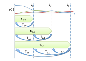
which reduces to the Markovian limit if all $\mathrm{T}$ vanish except for the tensors corresponding to a single timestep $\mathrm{T}_{n+1,n}$. Illustrated in Fig.(1), this expression establishes the relationship between the maps $\mathcal{E}_{n}$ and the tensors $\mathrm{T}_{n,m}$, and allows us to transform the dynamical mapping defined in Eq.(1) into a dynamical propagation,

$$\rho(t_{n})=\sum_{k=0}^{n-1}\mathrm{T}_{n,k}\rho(t_{k}).$$ (3)

In a sense, we regard the non-Markovian effect as time correlations in the quantum trajectory, and encode the correlation between any pair of time slices $t_{k}<t_{n}$ in the tensor $\mathrm{T}_{n,k}$, so that $\mathrm{T}_{n,k}\rho\left(t_{k}\right)$ corresponds to the component of $\rho\left(t_{n}\right)$ that is conditioned on $\rho\left(t_{k}\right)$. As in Eq.(1), the summation over all the possible components determines the density matrix at time $t_{n}$.

Figure 1: Diagram of the relationship between the dynamical maps $\mathcal{E}_{k}$ and the transfer tensors $\mathrm{T}_{k,r}$. While the dynamical map propagates any initial condition to a later time $t_{k}$, the transfer tensor $\mathrm{T}_{k,r}$ quantifies the direct correlation of the state of the system at time $t_{k}$ and the state at time $t_{r}$.

The formulation presented above is general, and will now be simplified by assuming time-translational invariance and finite time correlation in the transfer tensor. Under certain assumptions, e.g. separable system-bath initial conditions and a time independent Hamiltonian, we may invoke time-translational invariance so that the transfer tensor is a function of the time difference only, $\mathrm{T}_{n,k}=\mathrm{T}_{n-k}$. This selects a unique time frame in the dynamics, related for instance to the initial pulse in ultrafast laser excitation. We note that the time-translational property applies in general only to the transfer tensor, whereas for the dynamical map it holds only under Markovian or unitary dynamics. The tensors may now be obtained from the set of dynamical maps in an iterative fashion. $\mathcal{E}_{1}$ corresponds to the Markovian part of the dynamical map, generated by the system Hamiltonian and the initial relaxation due to the system-bath interaction, and we define $\mathrm{T}_{1}\equiv\mathcal{E}_{1}$. The second map $\mathcal{E}_{2}$ contains the effect of two sequential Markovian steps, $\mathcal{E}_{1}^{2}$. Any deviation of $\mathcal{E}_{2}$ from $\mathcal{E}_{1}^{2}$ arises from the memory effect of the non-Markovian bath and is encapsulated in the transfer tensor $\mathrm{T}_{2}\equiv\mathcal{E}_{2}\text{\textendash}\mathcal{E}_{1}\mathcal{E}_{1}=\mathcal{E}_{2}-\mathrm{T}_{1}\mathcal{E}_{1}$. Similarly, $\mathcal{E}_{3}$ contains the correlation between $t_{0}$ and $t_{3}$, and $\mathrm{T}_{3}\equiv\mathcal{E}_{3}\text{\textendash}\mathrm{T}_{1}\mathcal{E}_{2}\text{\textendash}\mathrm{T}_{2}\mathcal{E}_{1}$. Following this procedure, one can iteratively extract past-present correlations from dynamical maps. Since the timespan of bath correlations in realistic systems is finite, one may define a cutoff $K$ such that $\mathrm{T}_{s}\rightarrow 0$ for $s>K$. In practice, one would define an accuracy threshold $\epsilon$ for some measure of the magnitude of the tensor (for instance, the trace norm). One would define the cutoff as the point where that measure falls below the threshold. This justifies the truncation of the sum in (3) at $k=K$. Therefore, the dynamics of a large class of quantum systems may be encoded in the finite set of transfer tensors $\mathrm{T}_{s}$ with $s\in\left\{1,\dots,K\right\}$ and the matrix propagation equation (3) for times $t_{n}>t_{K}$ can be regarded as a tensor multiplication method,

$$\rho(t_{m})=\left(\begin{array}[]{cccc}\mathrm{T}_{1}&\mathrm{T}_{2}&\ldots&\mathrm{T}_{K}\end{array}\right)\left(\begin{array}[]{c}\rho(t_{m-1})\\ \rho(t_{m-2})\\ \vdots\\ \rho(t_{m-K})\end{array}\right),$$

which is the non-Markovian extension of time-local dissipative quantum dynamics and defines our Transfer Tensor Method (TTM) for propagation.

The TTM equation completes the basic 4-steps scheme: generate short-time trajectories numerically or experimentally, learn from short-time trajectories to extract the dynamical maps in Eq.(1), use Eq.(2) to derive the transfer tensors from the map, and evolve the density matrix to arbitrarily long time according to Eq.(3). This procedure is completely general, and applies to any system or bath, continuous or discrete. Yet, for simplicity of the benchmarking, we will use the numerical example of the spin-boson model below.

Scaling and error estimation.— With TTM we hope to address a challenge faced by many numerically exact simulation methods of open quantum systems: one can typically recognize an unfavorable exponential scaling of resources with the number of simulated time-steps. In the case of stochastic or Monte Carlo methods, an exponentially larger sample size is required for longer simulations. Renormalization methods Koch et al. (2003); Hughes et al. (2009); Gualdi and Koch (2013) require an ever increasing representation of the bath as time increases. The hierarchy of equations of motion Ishizaki and Tanimura (2005) is limited to the Drude-Lorentz bath and is characterized by a factorial scaling with the increase of the hierarchy levels. In the case of QUAPI Makri and Makarov (1995) or any other deterministic approach based on a path integral formulation, each path requires explicit storage and the tensor scales exponentially like $D^{2(K+1)}$ for a Hilbert space of dimension $D$ and a truncation $K$ on the memory kernel. The TEDOPA Prior et al. (2010) method has a more favorable scaling, but the size of its representation increases with temperature and time. In all the cases mentioned, this time-dependent scaling is usually in addition to the one depending on the system size. A remarkable aspect of the tensor multiplication method is the linear scaling of the storage requirements, since the total size of the set of transfer tensors is $KD^{4}$. Thus, by combining our method with an exact simulation one manages to reduce the required resources for long-time simulation by a significant amount. Based on this, our method is especially suitable for large systems, strong damping, and long memory time. Another useful aspect of the scheme is the direct relationship between the magnitude of the elements of the last tensor and the accuracy of the propagation. Despite being system specific, a reasonable upper bound for the error $e$ associated with the truncation at level $K$ is represented by some norm measure of the first neglected correlation operator, i.e. $e\simeq|T_{K+1}|$. This error accumulates in a multiplicative fashion. Since $K$ can be arbitrarily chosen, the error of the long time prediction can be reduced at will. It is worth noting that this method is deterministic and is therefore not affected by the so-called “sign problem” of Monte Carlo and stochastic propagation methods.

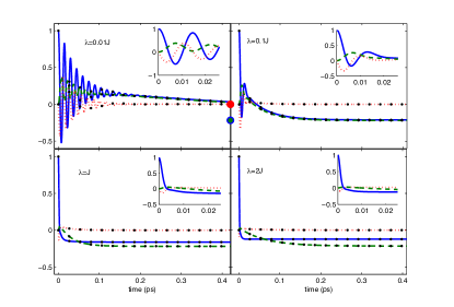
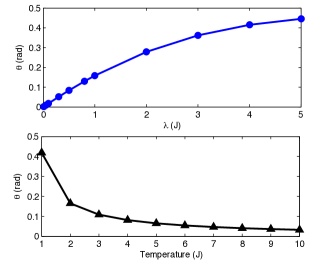
Examples of propagation.—We now demonstrate the applicability of the proposed method with two examples. To begin with, trajectories of a biased two level system (TLS) with exponentially decaying noise have been generated using the hierarchy method Ishizaki and Tanimura (2005) and the TTM. The frequency difference of the TLS is $\omega_{0}=100\mathrm{cm^{-1}}$ and the intrinsic coupling is $J=\omega_{0}$. The TLS couples off-diagonally to a harmonic bath of temperature $T=300K$, a characteristic frequency of $\gamma=J$ and a variety of system-bath couplings ranging from $\lambda=0.01J$ to $\lambda=2J$. As shown in figure (2), after the initial learning period shown in the insets, TTM successfully reproduces the transient dynamics of the density matrix until it reaches equilibrium. The different values of system-bath couplings are chosen such that the crossover between underdamped to overdamped dynamics is illustrated: while the first panel with $\lambda=0.01J$ contains oscillatory dynamics at short time, these progressively disappear with increasing $\lambda$ until no trace of coherent oscillations can be observed for $\lambda=2J$. It is worth noting that the composition of the equilibrium state varies with $\lambda$ due to quantum noncanonical statistics Lee et al. (2012); Moix et al. (2012). This effect is correctly reproduced by our method, which indicates its suitability to predict long time dynamical features with high accuracy. As the second example, we have further explored this effect quantitatively using a measure of the deviation from the canonical equilibrium distribution as defined in Lee et al. (2012): the Bloch sphere angular distance $\theta$ between the canonical distribution eigenbasis and the non-canonical one. Figure (3) explores the deviation $\theta$ as a function of the system-bath coupling $\lambda$ and the temperature $T$. The equilibrium entanglement with the bath increases with the strength of the interaction, which results in an increasing deviation from the canonical equilibrium that is specific to quantum systems. For a strong enough system-bath coupling, the non-canonical distribution reaches the eigenbasis of the system-bath interaction operator and the deviation angle saturates. In the present case, the saturation angle corresponds to $\frac{\pi}{4}$ radians. In contrast, thermalization supresses entanglement, which explains the decrease of deviation from the canonical equilibrium with increasing temperature. The equilibrium density matrix returns to the Boltzmann distribution in the high-temperature limit. It is evident from these two examples that TTM is suitable for long time simulation of dissipative quantum systems for which existing methods are not efficient or practical. This opens up a new possibility for exploring a plethora of previously unaccessible dynamical regimes.

Figure 2: Numerically exact simulation with the hierarchic method (lines) and prediction with TTM (dots) of the density matrix elements of a two level system under the influence of a Drude-Lorentz bath for different values of the system-bath coupling $\lambda$. Blue (solid) lines correspond to $\left(\rho_{11}-\rho_{22}\right)$, green (dotted) lines to $Re\left\{\rho_{12}\right\}$ and red (dashed) lines to $Im\left\{\rho_{12}\right\}$. The inset of every plot shows the corresponding learning period for the initial condition $\rho_{11}(0)=1$. The system-bath parameters are $T=300K$ ($k_{B}T\simeq 2\hbar J$), and $\gamma=J$, with $J=100cm^{-1}$. The equilibrium state for the case of $\lambda=0.01J$ is shown with colored dots on the axis.

Figure 3: Deviation $\theta$ from the canonical distribution as a function of the system-bath coupling $\lambda$, the cutoff frequency $\gamma$ and the temperature $T$. The learning period spans the first 25fs of the dynamics. The coupling is $J=100cm^{-1}$ and the cutoff frequency is $\gamma=5J$. In the upper panel $k_{b}T=2\hbar J$ and in the lower panel $\lambda=J$.

Extraction of the Nakajima-Zwanzig equation.—A unique aspect of the TTM approach is the possibility of using the complete information obtained via the dynamical maps to generate the equation of motion and the associated dynamical operators. Earlier, simple methods have been used to determine the Hamiltonian and the Markovian decoherence Humble and Cina (2006). Here we demonstrate that the non-Markovian nature of the dynamics, i.e. the memory kernel and consequently the correlation function of the environment, can also be rigorously determined. For this reason, it is useful to relate the non-Markovian dynamical maps to the physical terms in the exact Nakajima-Zwanzig formalism Breuer and Petruccione (2007); Nakajima (1958); Zwanzig (1960), where the evolution of an open quantum system with separable initial conditions can be expressed exactly in the form of the equation

$$\dot{\rho}(t)=-i\mathcal{L}_{s}\rho(t)+\int_{0}^{t}\mathcal{K}(t,t^{\prime})\rho(t^{\prime})dt^{\prime}.$$ (4)

Here, $\mathcal{L}{}_{s}$ is the Liouvillian of the system alone, and $\mathcal{K}(t,t^{\prime})$ is the memory kernel due to the system-bath interaction (Breuer and Petruccione, 2007). This equation can be seen as the continuous limit of Eq. (3). Thus, by comparing the time–convoluted kernels, we can easily identify,

$$\mathrm{T}_{k,n}=(1-i\mathcal{L}_{s}\delta t)\delta_{k,n+1}+\mathcal{K}_{k,n}\delta t^{2}.$$ (5)

Here $\mathcal{K}_{a,b}=\mathcal{K}(t_{a},t_{b})$ and $\delta_{a,b}$ is the Kronecker delta. This identity not only elucidates the physical motivation for using the transfer tensors $\mathrm{T}_{k}$ instead of the dynamical maps $\mathcal{E}_{k}$ in the numerical propagation of the density matrix, but also suggests using TTM to evaluate the memory kernel. Specifically, we extract the dynamical maps from the short-time dynamics, use Eq.(2) to transform the maps into tensors, and then identify the tensors with the system Hamiltonian and memory kernel in Eq.(4).

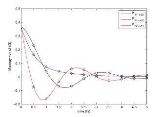
An example that illustrates this approach is shown in Fig.(4), where the memory kernel is plotted as a function of time for the spin-boson model. The numerical results are extracted from a hierarchy simulation of short-time trajectories under the influence of a Drude-Lorentz bath. As the benchmark, we compare the simulated memory kernel with the prediction from path integral calculations using the Feynman-Vernon influence functional and find perfect agreement. The ability to generate the transfer tensors $\mathrm{T}_{k}$ directly from the influence functional for large-scale simulations of quantum dissipative systems (up to hundreds of excitonic states) will be presented elsewhere.

The connection to the memory kernel further specifies the conditions under which time-translational invariance can be assumed. If (i) the total Hamiltonian is time-independent, (ii) the initial total state is a product state and (iii) the initial state of the environment is a stationary state, then the memory kernel depends only on the difference of its arguments, i.e. $\mathcal{K}(t,t^{\prime})=\mathcal{K}(t-t^{\prime},0)$; see §5.1 in Rivas and Huelga (2011), also Breuer and Petruccione (2007); Cao (1997). These conditions are hence directly related to the time-translational invariance of the transfer tensors.

Figure 4: Real parts of non-zero elements of the memory kernel as a function of time. The nonzero elements are $\mathcal{K}_{11\rightarrow 11}=-\mathcal{K}_{11\rightarrow 22}$, $\mathcal{K}_{22\rightarrow 22}=-\mathcal{K}_{22\rightarrow 11}$ and $\mathcal{K}_{12\rightarrow 21}=-\mathcal{K}_{21\rightarrow 21}=-\mathcal{K}_{12\rightarrow 12}=\mathcal{K}_{21\rightarrow 12}$. The solid lines represent the matrix elements of the memory Kernel extracted by applying TTM to a hierarchy simulation of a symmetric two level system with coupling $\Omega$. The dots are the values corresponding to the analytical prediction. The dissipative system is characterized by the parameters $\lambda=0.25\Omega$, $\gamma=0.05\Omega$ and $\beta\Omega=4.79$.

Conclusion.—We have presented a strategy based on non-Markovian dynamical maps to process the relevant information encapsulated in the trajectory of an open quantum system. This information can be used to learn about the underlying dynamics of the system in order to generate a set of transfer tensors for propagation to longer time scales. Applications of TTM to short-time trajectories clearly demonstrate the dynamic transition from coherent oscillations to incoherent transfer and accurately predict the non-canonical equilibrium distributions. Further, the transfer tensor method can be used to reconstruct the relevant dynamical operators of the system such as its Hamiltonian and memory kernel, by identifying the tensors with the Nakajima-Zwanzig equation. Due to its adaptability and scalability, the proposal not only constitutes a pedagogic approach to the description of open quantum systems but also stands out as a promising technique to extend the timespan of simulating quantum trajectories.