A Flux Scale for Southern Hemisphere 21cm EoR Experiments
Abstract
We present a catalog of spectral measurements covering a 100–200-MHz band for 32 sources, derived from observations with a 64-antenna deployment of the Donald C. Backer Precision Array for Probing the Epoch of Reionization (PAPER) in South Africa. For transit telescopes such as PAPER, calibration of the primary beam is a difficult endeavor, and errors in this calibration are a major source of error in the determination of source spectra. In order to decrease reliance on accurate beam calibration, we focus on calibrating sources in a narrow declination range from -46° to -40°. Since sources at similar declinations follow nearly identical paths through the primary beam, this restriction greatly reduces errors associated with beam calibration, yielding a dramatic improvement in the accuracy of derived source spectra. Extrapolating from higher frequency catalogs, we derive the flux scale using a Monte-Carlo fit across multiple sources that includes uncertainty from both catalog and measurement errors. Fitting spectral models to catalog data and these new PAPER measurements, we derive new flux models for Pictor A and 31 other sources at nearby declinations, 90% are found to confirm and refine a power-law model for flux density. Of particular importance is the new Pictor A flux model, which is accurate to 1.4% and shows, in contrast to previous models, that between 100 MHz and 2 GHz, the spectrum of Pictor A is consistent with a single power law given by a flux at 150 MHz of 3825.4 Jy, and a spectral index of -0.760.01. This accuracy represents an order of magnitude improvement over previous measurements in this band, and is limited by the uncertainty in the catalog measurements used to estimate the absolute flux scale. The simplicity and improved accuracy of Pictor A’s spectrum make it an excellent calibrator in a band of importance to experiments seeking to measure 21cm emission from the Epoch of Reionization.
Subject headings:
dark ages, reionization, first stars — catalogs — instrumentation: interferometers1. Introduction
Numerous radio telescopes are now exploring the prospects for using measurements of highly redshifted 21cm emission to inform our understanding of cosmic reionization in the redshift range , corresponding to radio frequencies below 200 MHz (see reviews in Furlanetto et al. 2006; Morales & Wyithe 2010; Pritchard & Loeb 2012). These include telescopes aiming to measure the global temperature change of 21cm emission during the Epoch of Reionization (EoR), such as the Compact Reionization Experiment (CoRE), the Zero-spacing Interferometer (Raghunathan et al., 2011) and the Experiment to Detect the Global EoR Signature (EDGES; Bowman & Rogers 2010), and interferometers aiming to measure the power spectrum of 21cm EoR emission, such as the Giant Metre-wave Radio Telescope (GMRT; Paciga et al. 2011, 2013)111http://gmrt.ncra.tifr.res.in/, the LOw Frequency ARray (LOFAR; Yatawatta et al. 2013; van Haarlem et al. 2013)222http://www.lofar.org/, the Murchison Widefield Array (MWA; Bowman et al. 2013; Tingay et al. 2013))333http://www.mwatelescope.org/, and the Donald C. Backer Precision Array for Probing the Epoch of Reionization (PAPER; Parsons et al. 2010; Pober et al. 2013)444http://eor.berkeley.edu/.
Given the immense science potential in detecting 21cm emission from the EoR, a great deal of research has focused on measuring the spectral and spatial variation of foreground emission in the 100-200 MHz band ( in the 21cm line), which dwarfs the 21cm signal by orders of magnitude (Furlanetto et al., 2006). In particular, the spectral properties of extra-galactic point-sources are important both because they are valuable calibration references and because they are strong foreground emitters that must be removed from 21cm EoR measurements. With the sparse availability of measured foreground properties in the 100–200-MHz frequency band over large areas of the sky (de Oliveira-Costa et al., 2008), continued foreground characterization is a vital step en route to any 21cm EoR detection. At these low frequencies, the Southern sky is much less well known than the North; catalog source fluxes at 150MHz are inaccurate at the 20% level for ° (Slee, 1995; Vollmer et al., 2005). Both PAPER and the MWA are located in the southern hemisphere at radio-quiet reserves being prepared for the upcoming Square Kilometre Array, and hence, the most extensive surveying work is now being conducted by the EoR experiments themselves (Jacobs et al., 2011; Williams et al., 2012; Bernardi et al., 2013).
One significant complication to improving the state of affairs in foreground characterization is that many 21cm EoR experiments, including LOFAR in the northern hemisphere, and PAPER and MWA in the southern hemisphere, are designed for drift-scan observations or steered via phased array. This design decision has largely been driven by the simplicity and cost-effectiveness of phased and/or correlated dipoles to achieve the aggressive sensitivity requirements for measuring the 21cm power spectrum of reionization (Parsons et al., 2012; Beardsley et al., 2013; Jelić et al., 2008). Adding to the challenge, these telescopes cover much wider fields of view (°) and bandwidths (% fractional) than traditional dish telescopes. Because they do not physically point, flux calibration for such arrays relies heavily on an accurate model of the primary beam response to correct for an the apparent flux scale that varies across the sky. This direction dependent gain is currently uncertain to 10% or higher (Pober et al., 2012), and comprises a large fraction of the 20% flux uncertainty between current telescopes (Jacobs et al., 2013).
In this paper, we set out to significantly improve the accuracy of spectral measurements between 100–200 MHz for a set of bright sources in the declination range -46° to -40° that are of particular value for southern-hemisphere 21cm EoR experiments such as PAPER and the MWA. Using the fact that, for this restricted declination range, sources transit through a nearly identical primary beam response pattern, we are able to avoid one of the most debilitating source of error in these measurements: the primary beam.
In §2 we provide some background on uncertainty in early EoR-band catalogs, and explain our choice of calibrators. In §3 we describe our approach for measuring source spectra with drift-scan observations and deriving an absolute flux scale from catalog data. In §4 we detail the instrumental setup, observations and analysis method followed. Sections 4.6 through 8 detail our approach for fitting a global flux scale and spectral models for each source. We use these fits in §5 to understand how well PAPER data agree with previous measurements and conclude in §6.
2. Background
Historically, the best Southern Hemisphere EoR band data were by Slee (1995) with Culgoora Circular Array555Known during daylight hours as Culgoora Radio Heliograph and various higher frequency measurements with Parkes. These data are typically uncertain to 20% or higher and provide little coverage of the EoR band beyond a single narrow-band data point. More recent surveys include narrow-band surveys by the GMRT 666http://tgss.ncra.tifr.res.in/ and Mauritius (Pandey & Shankar, 2005), a deep survey of the region near Hydra A by the 32 antenna MWA prototype (Williams et al., 2012) and a wide field survey by PAPER, also with 32 elements (Jacobs et al., 2011). Several sub-channels were provided in the Williams catalog, though with 60-80% error bars —large compared to the 30% uncertainty on their wide band measurements. The latter cover the band and spatial scales relevant to EoR measurements but are limited by the accuracy of the primary beam (Jacobs et al., 2013) as well as the lack of precise in-band flux calibrators.
The response of the primary beam is of critical importance to EoR measurements. Differences between the polarization responses cause leakage of polarized signals into the total intensity measurement possibly corrupting the EoR power spectrum (Moore et al., 2013). The primary beam shape is also critical to measuring and subtracting foregrounds (Bernardi et al., 2013; Sullivan et al., 2012; Morales et al., 2012) a process which, to be effective, must be done to better than 1% precision for the brightest sources Liu et al. (2009); Bowman et al. (2009) . A method for decoupling uncertain fluxes from the uncertain beam has been described by Pober et al. (2012). In simulation the method was able to achieve 3 to 10% accuracy in measuring the primary beam, depending on the number of antennae and other variables. In particular, it emphasized the need for many repeated measurements of each alt-az pointing, which in that case were found by assuming 180° symmetry. Further investigation is under way to improve and implement this method and would be greatly aided by the availability of precise flux measurements unaffected by primary beam uncertainty.
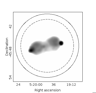
EoR measurements by PAPER and the MWA in the southern hemisphere have focused on the coldest regions where galactic foregrounds are minimal, with the majority of possible observing time falling around RA=4h,Dec=-30. The brightest and least-resolved calibrator in this region is Pictor A (5h19m49.1,-45d46m45.0). Pictor A is a nearby FR-II type radio galaxy similar to Cygnus A. At 400Jy, Pictor is bright and sufficiently distant from other bright sources to make it eminently suitable as both a phase and flux calibrator. Its apparent size of 8′ is smaller than the scales being probed by current EoR instruments, making it suitable for precision calibration, with only a modest level of resolution effects. However, like most other sources, precise flux measurements in the EoR band are not available. The previous best EoR band measurement is uncertain to 12% and appears to imply spectral flattening in the EoR band (Perley et al., 1997).
Establishing an accurate spectrum for Pictor A is of particular importance for PAPER — a dedicated EoR experiment that employs drift-scanning, dual-polarization dipole antennas tuned for efficient operation over a 120–170-MHz band. PAPER is located in the South African Karoo desert on the Square Kilometer Array South Africa (SKA-SA) reserve, 100km north of the small town of Carnarvon. The PAPER array has grown from 16 elements deployed in early 2009 to a 64-element imaging array in 2011 (see Figure 2). Since November 2011 it has been arranged in a maximally redundant grid configuration to make deep power spectral integrations (Parsons et al., 2012). Though highly sensitive as a power spectrum instrument, the maximally redundant array has a broad point spread function in the image domain. This severely limits the number of sources which may be used for flux calibration. Drift scanning across the sky with a 45° FWHM primary beam, there are very few unresolved, bright sources which are far from the galactic plane. Pictor A is bright and well enough separated from other emission to dominate the visibilities for a good fraction of the EoR observing season, making it a desirable source to use for flux calibration.
3. Approach
In this section, we describe our general approach to controlling the impact of beam model errors on measured spectra derived from drift-scan observations of Pictor A and a selection of known, bright sources. Our approach uses a set of “source tracks” as a function of frequency and time. Each source track is a beam, formed by phasing measured visibilities toward known source locations as they drift through the primary beam, and summing over antenna pairs, as described in §4.3. Since sources fall at different positions within the primary beam, it is generally not possible to relate the fluxes of sources at different positions to one another without an accurate beam model. To date, the accuracy of source flux measurements in the southern hemisphere in the 100–200 MHz band have largely been limited by the accuracy of these beam models.
We mitigate this problem by selecting sources within a narrow declination range, so that source tracks represent nearly identical cuts through the beam response pattern. Using this fact, the relative amplitudes of sources can be deduced with minimal reliance on an accurate beam model. In our analysis, a prior beam model is only necessary for extrapolating across a narrow declination range (we estimate the errors associated with this extrapolation in §4.7), and for approximating optimal inverse-variance weighting when averaging over source tracks to determine a single spectrum.
This approach addresses several sources of error that were identified in Jacobs et al. (2013) as originating from uncertainty in the primary beam model. First, under most imaging schemes, each source flux is measured at just a few points in the primary beam. As errors tend to vary across the beam it is often difficult to decouple flux uncertainty from beam uncertainty. Using the drift scan-beamforming technique, each source is measured thousands of times at a variety of different primary beam values to provide a complete sample of the flux variance due to primary beam variation. Second, the flux calibration was found to vary over the sky due to the dual uncertainties of primary beam response and prior catalog. To reduce our exposure to flux calibration variation, we limit our observations to sources passing within 5° of pointings which we can directly calibrate to a single reference source. A third limitation, identified in Williams et al. (2012), was the increase of uncertainty towards the edge of the beam. To minimize our sensitivity to both beam and noise uncertainty, we weight the source track by an additional factor of the primary beam model.
The remainder of the analysis in this paper relates to calibrating the relative source amplitudes that we establish to an absolute flux scale as a function of frequency. Given the shortcomings of existing in-band measurements of sources in the southern hemisphere, we must bootstrap this flux scale from an ensemble of calibrator sources that exhibit simple power-law spectra. As described in §4.7, this proceeds by first using a single calibrator to set the relative amplitudes of spectral channels, and then using several sources, extrapolating across a large set of measurements between 70 MHz and 2 GHz, in a Markov-Chain Monte Carlo simulation to establish an absolute flux scale for the measured spectra.
3.1. Source Selection
As PAPER is a drift scan instrument, each declination describes a distinct path through the primary beam. The flux time series of a beamform provides a detailed sample of the primary beam relative to the peak of the trace, however, a model is still required to calibrate between declinations. Below we argue that by averaging over long tracks, we minimize our susceptibility to localized primary beam error and find that limiting our source selection range to within a declination range of 5° around a calibrator is a good compromise. In §8, we estimate the error resulting from this limited scope application of the primary beam model.
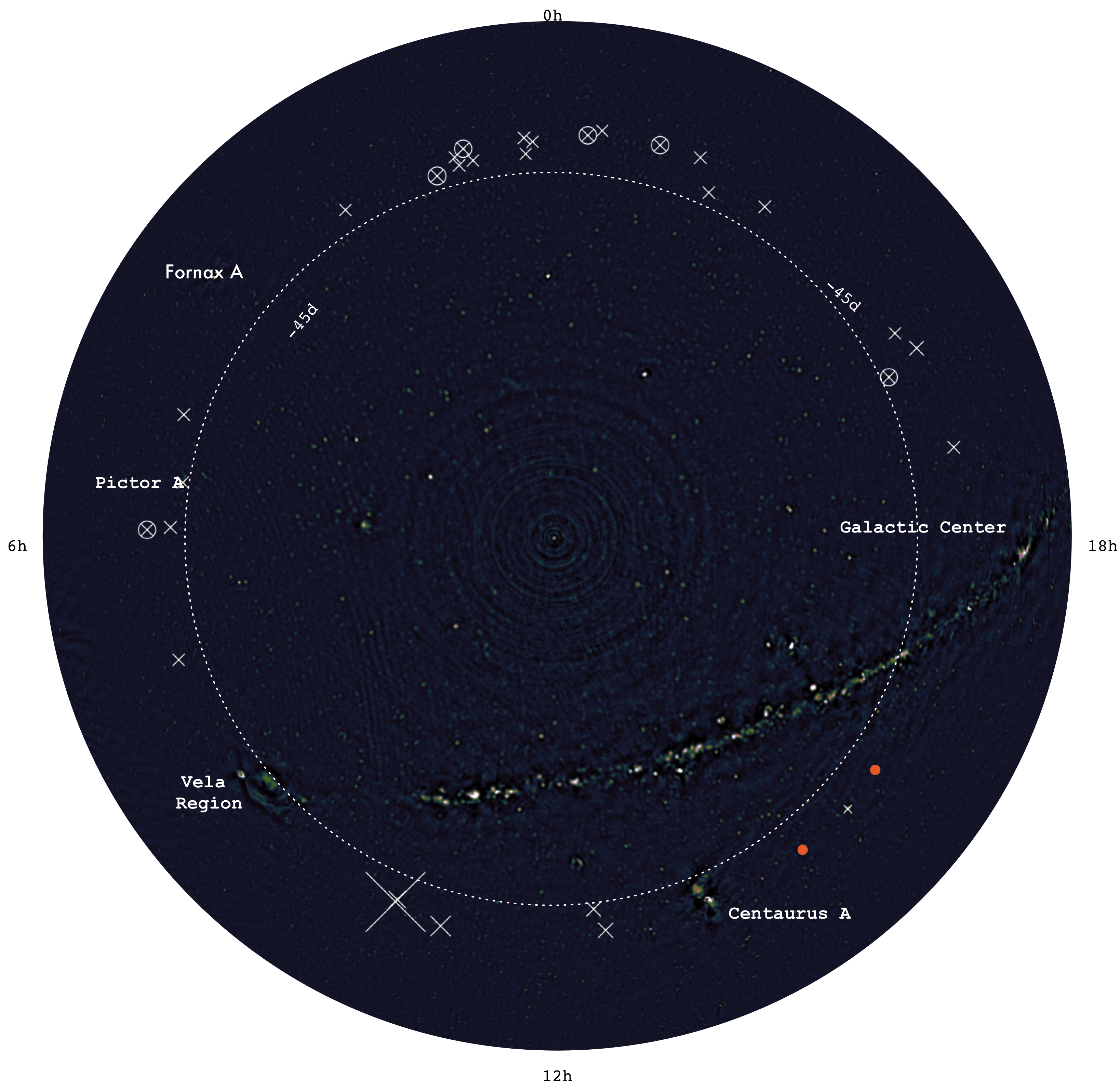
We choose sources from the Molonglo Reference Catalog (Large et al., 1981, MRC) that are within 5° in declination of a common calibrator (J2331-416), and more than 10° from the galactic plane and Centaurus A. We limit the flux extrapolated from 408MHz to be greater than 10Jy, assuming a power law spectral index of -1.777Most radio sources in this band have power law spectra and a typical spectral index of . This selection contains 32 sources in a narrow stripe that passes through the majority of the southern EoR fields. See Figure 1 for a map of the sources relative to the galactic plane and other structure as mapped by PAPER using the same observations presented here and Table 1 for a complete listing of names and positions.
3.2. Analysis Overview
The spectra reported here are measured by beam-forming — phasing the visibilities to the target location and summing over baselines to produce a spectral time series of “perceived” flux . We define a perceived flux as the true source flux density, , illuminated by the true beam pattern :
| (1) |
where is a function of time because the observations are taken as a drift scan. The desired source spectrum is then isolated from neighboring sources by delay filtering (Parsons & Backer, 2009). We then average the spectrum in the time domain, weighting by a model of PAPER’s primary beam response (); as the perceived flux is already weighted once by the true beam , this weighted sum is an effective approximation of inverse-variance weighting (Pober et al., 2012). Mathematically, our estimated source flux density is given by:
| (2) |
where the subscript indicates a model beam, and the without subscript is the true flux density of the source. The net time integrated, weighted beam response is purely a function of declination . The rate at which this factor changes with declination defines the declination range over which our calibrator source can be used to set the gain scale of the observations. To simulate this affect we multiplied a measurement of the primary beam (Pober et al., 2012) by electromagnetic simulations (Parsons et al., 2010) and find that diverges slowly with declination, with a maximum of 10% over 5° of declination range. Thus, to first order, we can use our calibrator source to calibrate sources within 5° of declination and remove most of the variation with declination. We estimate this spectral dependent at a reference declination of 41°36′ using (J2331-416), fitting a spectral index model to the catalog data points below 2GHz. This levels the bandpass due to spectral dependence of the primary beam, and allows us to place our measured source flux estimates on approximately the same flux scale. Finally we average the spectra from a resolution of 400kHz to 10MHz bins, adding the individual errors in quadrature for our uncertainty.
At this point we have a set of spectra that have been calibrated relative to each other to the best of our ability. Now they must be put on a global flux scale. Meanwhile, our error estimate does not include an estimate of the flux calibration error. To address both points we fit for a global flux scale that incorporates the best available catalog data. These catalogs have all been set, as best as possible, to the Baars et al. (1977) scale to which all other points are tied. Using a Bayesian analysis we compute the variation in the flux scale implied by comparing many sources to prior catalog models. By including sources from across the RA/Dec range, the variation in this flux scale fit estimates the overall uncertainty in flux resulting from primary beam or prior catalog uncertainty. This folds in the error due to extrapolation beyond the frequency range of the Baars scale which is technically limited to 300MHz and above.
4. Data Reduction
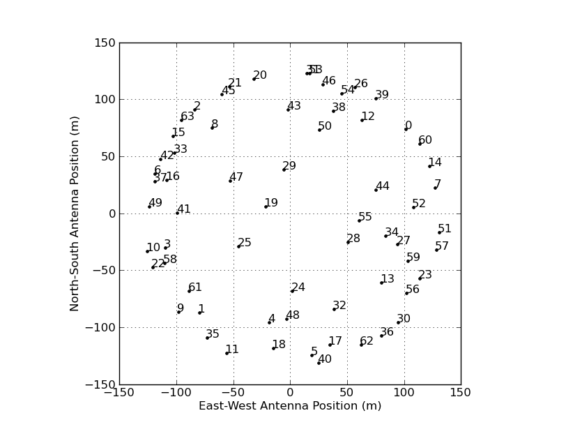
Measurements are derived from observations using two nights on the east-west dipole arms of 64 PAPER antennas deployed in a minimum-redundancy imaging configuration (see Figure 2) at the Karoo Radio Observatory site in South Africa. A100-200MHz band was correlated with 2048 frequency channels and integrated for 10.7 seconds before visibilities were stored. Observations included here on July 4, 2011, running from JD2455748.17 to JD2455748.72. and October 17, 2011 running from JD2455852.2 to JD2455852.6. In both seasons two antennas were omitted owing to malfunctioning signal path. This 20 hour long combined dataset provides observations provides near complete hour angle coverage for the entire 24 hours of Right Ascension. The July portion of the dataset comes from the same observing campaign described by Pober et al. (2013) and Stefan et al. (2013).
4.1. Data Compression
In pre-processing, we use delay/delay-rate (DDR) filters (Parsons & Backer, 2009) to identify radio-frequency interference (RFI) events, and as part of a data compression technique that reduces data volume by over a factor of 40. A more detailed description may be found in Appendix A of Parsons et al. (2013), which uses the same compression method on PAPER power spectrum observations. Here we summarize the process.
First, we remove known RFI transmission bands and analog filter edges, and then flag outliers in the frequency and time derivative at 6 to remove RFI events. Next, we suppress sky-like emission by applying a DDR filter to remove delays and delay-rates within the horizon limit of a 300-m baseline (the maximum length of any PAPER baseline). We derive a second set of RFI flags by masking 4 outliers in these residuals and apply these flags back to the unfiltered data. Finally, we compress the data by applying a DDR filter preserving emission within the horizon limit of a 300-m baseline, deconvolving to suppress flagging artifacts, and down-sampling the result in time/frequency domain to the critical Nyquist rate of the DDR filter. The result is that the 2048 original frequency channels become 203, and the 60 original time samples per 10-minute file become 14.
4.2. Per-Antenna Gain Calibration
Small time- and antenna-dependent gain variations time introduce significant systematic effects that degrade instrument performance. Temporal variations are dominated by changes in ambient temperature. We use measurements of ambient temperature versus time on the balun amplifier of a fiducial antenna and near receiver amplifiers to divide out the predicted gain variation versus temperature that these amplifiers are known to exhibit. Inspecting the auto correlations we find that the net antenna temperature gain coefficient (-0.042 dB/C) found in previous laboratory (Parashare, 2011) and early field measurements (Pober et al., 2012) did not appear to remove all temperature variation. To revise the temperature coefficient we use the October observations, when the temperatures remained nearly constant, as a reference.
Comparing the average ratio between the July and October autocorrelations to their temperature difference (Figure 3) we find that the two are highly correlated with a best fit temperature coefficient of (-0.058 dB/C). As we see in Figure 4, this removes a significant amount of disagreement between the two nights, with the peak difference decreasing from 18% to 3%.

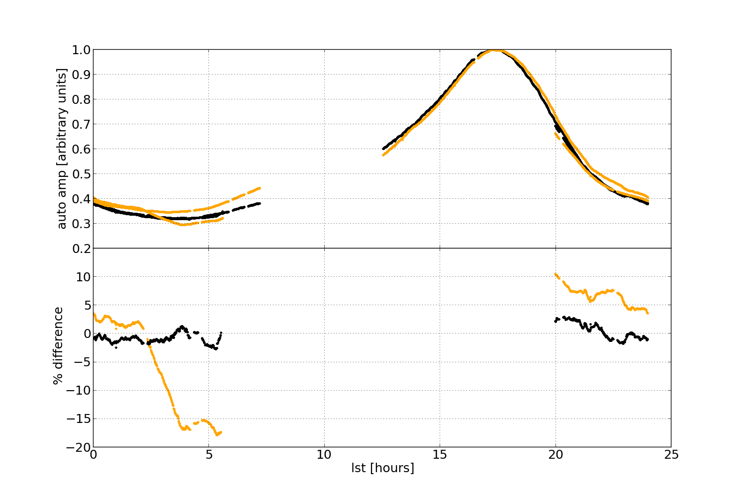
. Note that the span of the data in the bottom fractional difference plot is limited to points occurring in both nights and does not cover the full range seen in the top.
Matching of relative gains and phases between antenna was done by fitting a per-antenna complex gain to portions of data which have easily modeled sky. This calibration is only relative between antennae, bandpass and absolute flux calibration comes after time and frequency averaging in sections 4.5 and 4.7. The antenna delays and amplitudes were found by fitting a point source visibility model to Centaurus A, Pictor A, and Fornax A. Each source is imperfectly modeled by a single point-source, but the solution differences are minimized by averaging over the three independent solutions. These same calibration solutions have been successfully applied in Pober et al. (2013) and Stefan et al. (2013). for power-spectrum analysis of foregrounds and imaging of Centaurus A, respectively.
The October per-antenna gains were found by computing the average ratio of the auto correlations against the July data. Delays were held constant as in Jacobs et al. (2011).
4.3. Beamforming
Spectral time-series are computed by beam-forming to the selected sky locations. A beam is formed by phasing baselines to the desired location and summing over baselines longer than 20 wavelengths.
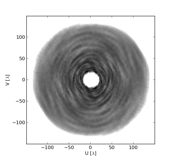
These complex spectra are then fringe rate filtered to remove spectrally smooth sources that deviate more than 0.1mHz from the fringe rate of the source in question (Parsons & Backer, 2009) (cf the LOFAR de-mixing approach (Offringa et al., 2012)) producing a time dependent spectrum with minimal side lobes. This is then averaged in time, weighting by a model of the primary beam as discussed above. The result is equivalent to a very long earth rotation synthesis image with a single image pixel. The weighted contributions from each baseline (the uv coverage) are shown in Figure 5. When combined with the filtering it is a robust and simple method for measuring spectra of unresolved sources.
4.4. Compensation for Resolution Effects in Pictor A
Not shown here are the weights interpolated from the Perley et al 330MHz map (Fig. 6) used to recover the total integrated flux of Pic which represent a few % change on the longest baselines.
The beam-forming method assumes the target is a point source. Our primary target, Pictor A, is slightly resolved by PAPER, and merits closer attention. Pictor A is a double-lobed radio galaxy with a main lobe separation of 7′. As we see in Figure 6, it is nearly unresolved by PAPER’s 15′ synthesized beam. However, given the high SNR of the observations, we see a 20% drop in flux on the longest (300m) baselines. We account for this by weighting baselines in the beamform step according to a model of structure observed by Perley et al. (1997) at 330MHz, which they found to be consistent with their more limited 74MHz images as well as the detailed high frequency maps. The normalized image is Fourier transformed and sampled at the desired uv spacing by spline interpolation. These samples are used to weight each baseline contribution in the baseline sum. The result is an estimate of the total integrated flux for Pictor A. Where the resolution is highest, at the top of the band, the net correction is 3%. At the bottom of the band, where the resolution size has grown to 19′, the correction is only 0.6%. The resulting spectrum is shown in Figure 7a.


4.5. Bandpass Calibration
The resulting set of spectra were then calibrated to a model of J2331-416 888Here we set the spectrum to Jy, , derived by a linear least squares fit to catalog measurements below 1GHz (Slee, 1995; Kuehr et al., 1981; Large et al., 1981; Burgess & Hunstead, 2006). Further calibration on top of this somewhat arbitrary calibration model is explored in detail below. to remove the residual bandpass from equation 2 caused by the net effect of the primary beam as discussed in section 3. This source was selected for its relatively high brightness, spectral smoothness and large quantity of available catalog data. Each source track has a slightly different sample profile resulting from different amounts of flagged data at each time and channel. To account for these differences in the bandpass calibration we build a set of calibration tracks that match the tracks for each source. Calibration of each source then proceeds with an optimally matched calibration spectrum.
4.6. Fitting a Power-Law Model to Spectra
There is a variety of prior data at multiple wavelengths to which we want to calibrate and then compare our measurements. Our method for doing both of these steps is to assume a basic spectral model relating the different catalog data points and fit for spectral model and gain parameters.
We estimate spectral model parameters and flux calibration in a Bayesian way by calculating and marginalizing the posterior probability of the catalog and new PAPER data. This method offers improved repeatability by specifying a single objective function that represents the quality of the model fit and naturally defines the errors on the parameters (Hogg et al., 2010). See Mackay (2003) or Sivia & Skilling (2006) for more on Bayesian analysis methods and an excellent astrophysical example by Press (1997). In brief, measurement errors are related to parameter model errors via the likelihood, which we can calculate, and the posterior, which we cannot. However, the posterior is theoretically well sampled by a Markov Chain Monte Carlo (MCMC) sampler, which selects parameter values at random, computes the likelihood of the model given the data and noise model, and accepts or rejects the step based on an outside decision factor unrelated to the data.
Here we use the emcee sampler by Mackay (2003) et al to generate chains of parameter values. The best fit model is the median of all the sampled parameter sets, while the volume containing a well defined fraction of samples sets the confidence limits. The oft quoted “1” probability level corresponding to a gaussian distribution contains 65% of the samples. In practice the contours are not gaussian. Here we choose a slightly more conservative probability level of 76%
To model the relationship between different wavelengths we assume a single spectral index which is the prevailing spectral energy distribution at low frequencies, though curvature or other deviation from a power-law is not uncommon.
When fitting models to the full catalog, we use the Vollmer et al. (2010) catalog which has been optimally cross-matched at the expense of excluding more data points. Meanwhile, the gain fit used a small sample of sources with spectra which meet our calibration criteria: more precision data available, brighter than most sources in the sample and far from any possibly confusing areas of the sky. By limiting ourselves to a small number of sources we are able to go include catalog points by hand, to avoid making the error of falsely including erroneously matched data points.
4.7. Approximating the Absolute Flux Scale
At the output of the beam forming and bandpass calibration step, the flux scale is tied to a model fit of the catalog values of J2331-416. The accuracy of this fit, and the implied uncertainty in the flux scale, limits the accuracy of the PAPER measurements. To refine the flux scale and estimate our flux scale uncertainty, we bootstrap a single global flux scale correction factor using 6 sources selected for their brightness, spectral linearity and data availability999Calibration sources: 2250-412,2331-416,1932-464,0103-453,0547-408,0043-424. To build a more complete spectral model we go beyond the data found in Vollmer et al. (2010) to include all spectral measurements below 2GHz found in the NED database 101010ned.ipac.caltech.edu: Accessed 1 April 2013. These additional catalog measurements are primarily by Parkes, and Molonglo (Kuehr et al., 1981) with the best precision coming from the Wills fluxes at 538 and 634 MHz (Wills, 1975). Where error bars are not given, we assume uncertainty of 25%.
Using the MCMC method we fit spectral index models to the catalog fluxes simultaneously with a global PAPER flux scale factor using an MCMC chain to calculate the log likelihood
| (3) | ||||
| (4) |
which samples the posterior probability of PAPER data () and catalog values () given a spectral index model for each source and a global flux scale factor (). Marginalizing over the fitted flux scales, we find the resulting flux scale distribution function which is shown in Figure 8. The 76% confidence limit on this flux scale, relative to the J2331-413 calibration, is dB, or a 1.54% multiplicative error on every calibrated PAPER measurement. This flux scale is applied to the PAPER spectra with the errors added in quadrature.

4.8. Fitting Spectral Models
Finally we compare all of our calibrated spectra to catalog measurements. Our method will be to first establish a best fit model to existing data, then add the PAPER data to the fit, and assess the degree to which the PAPER data is supported by prior measurements (accuracy), and the reverse, the degree to which PAPER offers an improvement in our knowledge of the spectrum (precision).
To establish a baseline model, we fit a spectral model to prior catalog data from the spectrally and spatially cross-matched meta-catalog by Vollmer et al. (2010) using the MCMC chain to sample the (log) likelihood which assumes Gaussian measurement errors
| (5) |
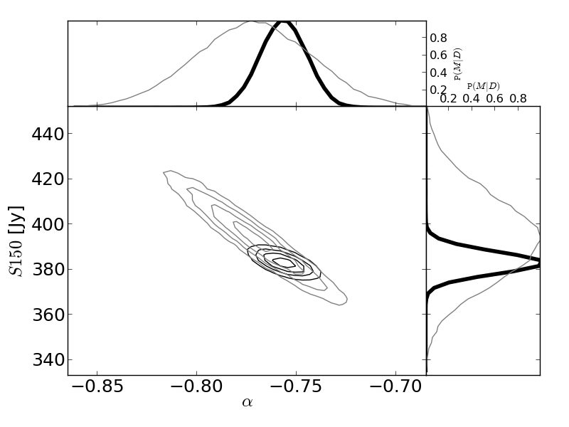
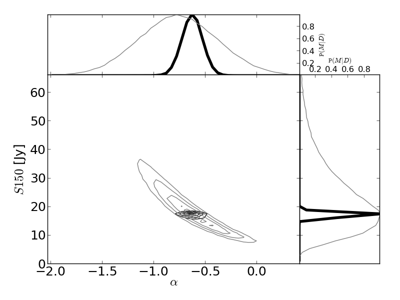
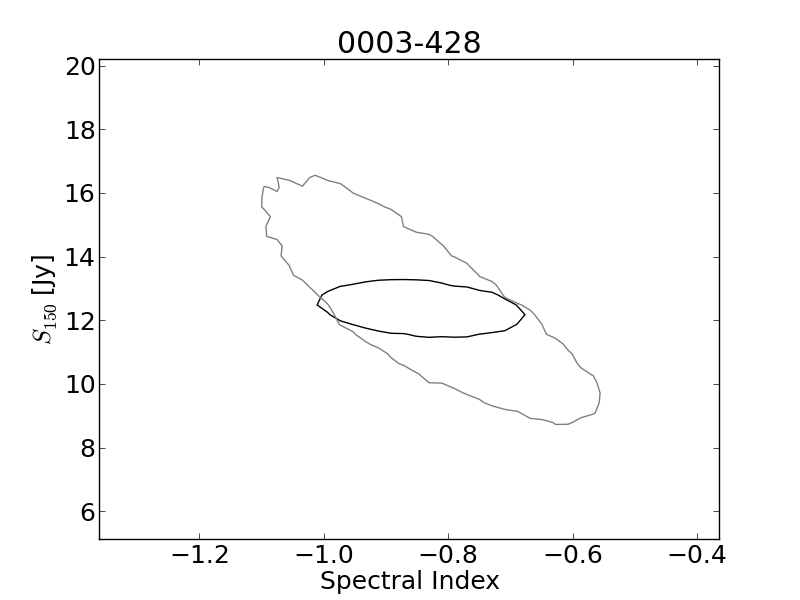
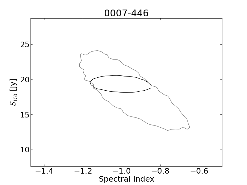
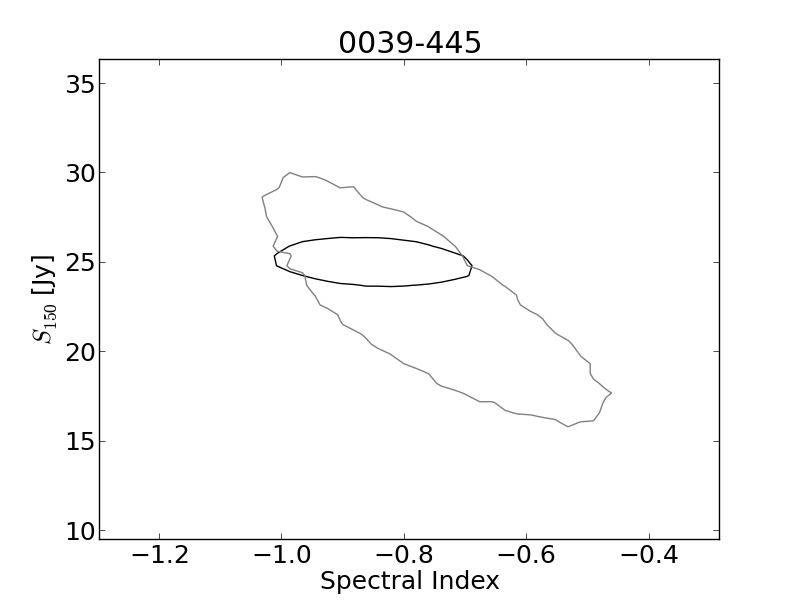
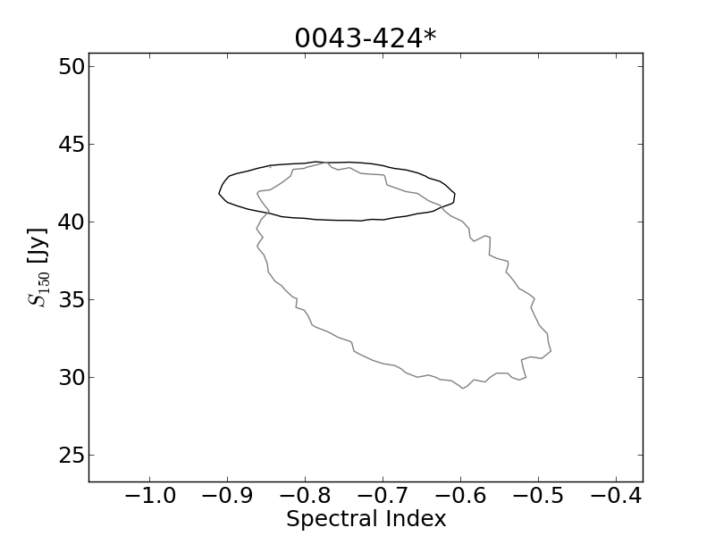
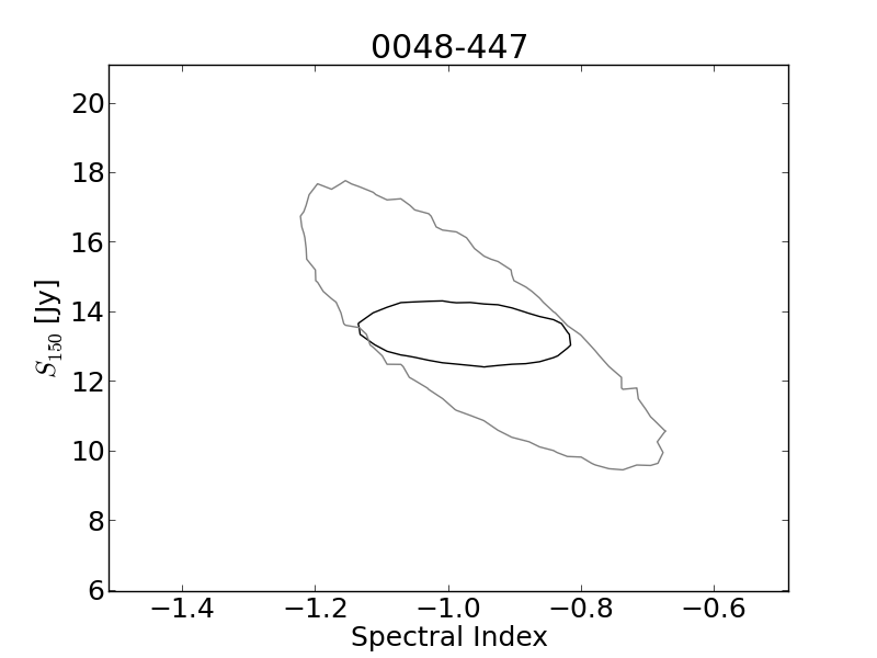
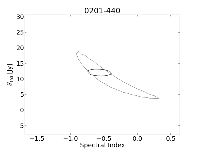
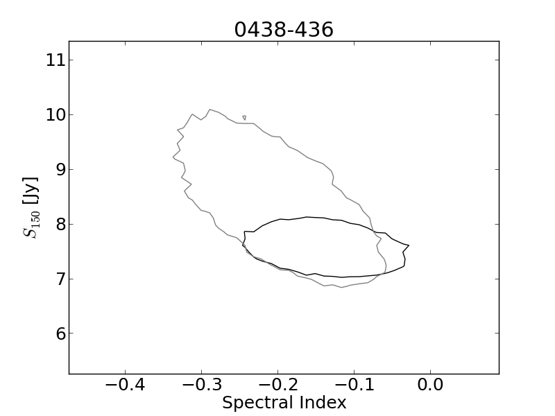
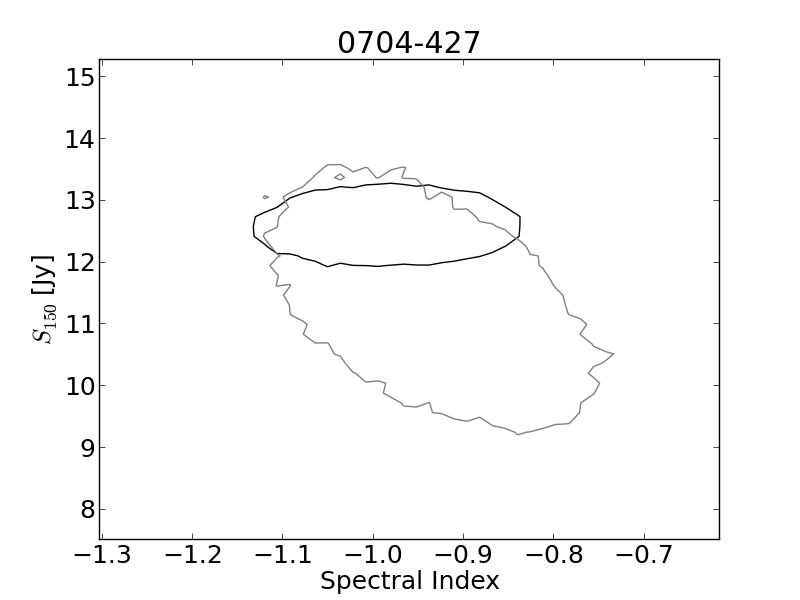
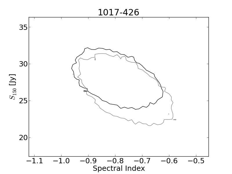
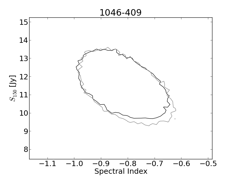
As when fitting the flux scale, we estimate the confidence interval of the resulting parameters as the boundary enclosing 76% of the samples. A detailed view of the resulting posterior is shown in grey on Figure 9. Most of the posteriors are characterized by steep sided, symmetric distributions. While many appear to have linearly correlated parameters, several display the classic banana shape associated with a non-linear correlation between parameters. For the rest of the sources we focus on the 76% confidence levels, plotting the 2D distributions in Figures 11 - 15, and listing the marginalized values in Table 2.
The fit is then performed again with both PAPER and catalog data, shown in black on the same Figures.
5. Results and Discussion
The majority of the 32 models fit using the new PAPER data were found to agree with models fit to past data and all but two are suitable for comparison. 0008-421 was not detected by previous PAPER observations and exhibits flattening at higher frequencies, most likely due to synchrotron self-absorption (Jacobs et al., 2011). Meanwhile, 1459-417 does not have enough measurements in the SPECFIND catalog on which to build a model for comparison. We exclude these two from further analysis.
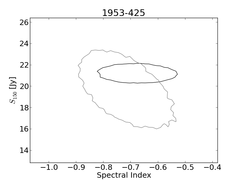
Inspecting the remaining 30 confidence contours we find that, for the vast majority (%), the PAPER measurements confirm the power law extrapolation from higher frequencies. The remaining 10% either A) have large PAPER error bars and therefore provide no new information or B) do not agree with the spectral index model. To understand where most measurements fall on this spectrum we numerically quantify the overall model improvement derived from the addition of the PAPER data as {fleqn}[0pt]
where the area is defined as the number of samples having posterior probability above 76%.
We quantify the fit precision increase as the change in the contour figure of merit, defined as the inverse area of the confidence contour. Meanwhile, catalog agreement is the fraction of the PAPER confidence interval that overlaps the catalog confidence interval. Thus, for example, in a PAPER fit that overlaps the catalog confidence contour by 41% but increases in precision (confidence area shrinks) by a factor of 3, the resulting improvement will be 0.123. This Improvement Index is included in the table of fit parameters (Table 2) and is used as the size scale on the map in Figure 1.
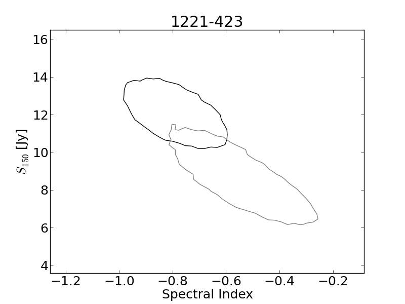
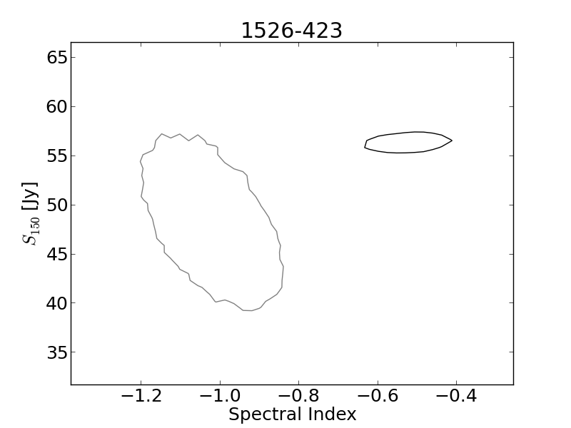
In these sources, the improvement index ranges from a maximum of 7.84 to -0.001. One source (1017-421) shows a slightly negative improvement, suggesting that PAPER data have added to uncertainty (see Figure 15), while two sources have exactly zero improvement, which indicates that the PAPER data have pulled the fit far from the model preferred by the catalog data (see Fig. 14 for details on these).
However, the vast majority of sources (90%) have positive improvement index, indicating strong confirmation of the extrapolated spectrum (see Figures 11 - 13). Pictor A is close to the top of this group with an improvement of 0.942 —only two sources show stronger confirmation. The flux model is 382 5.4Jy, a fractional error of 1.4%.
This represents an order of magnitude improvement in the accuracy of this primary flux calibrator. In fact the uncertainty is so small that it pays to consider its reasonableness. First consider that we have fit the model to many data points, including 7 measurements (5 PAPER, 2 Wills) accurate to 3%. If the errors were completely Guassian the net error would be %. Consider also that, where most surveys might include on the order of ten independent measures of a bright source from different facets to arrive at a 5 to 20% uncertainty, we have included thousands of independent measurements over the full horizon to horizon transit, while carefully controlling for systematic variation and resolution affects.
6. Conclusion
This paper presents a set of total flux measurements at multiple frequencies within a 100–200-MHz band, providing an absolute flux calibration for southern hemisphere EoR studies, as well as a modest set of verification fluxes for other sources suitable for constraining future primary beam studies. We have provided a measurement of Pictor A with enough precision to confirm a linear spectral index between 150 and 600MHz. We apply the same filtered beamforming method to measure the spectra of bright sources with similar primary beam response.
The measurements provided here are the first calibrated, broad-band spectra to cover the EoR band. Existing EoR band measurements are accurate to 20% implying a 40% uncertainty in the absolute power spectrum level. The PAPER Pictor A spectrum is found to be accurate to 3%, a factor of 7 improvement over previous EoR-band measurements.
This uncertainty includes the variation in each PAPER measurement (1%), variation between sources and the errors resulting from extrapolating the Baars et al. (1977) scale beyond its original range. These last two are found simultaneously by fitting the spectral extrapolations of several flux calibrators at once and account for about half of the error. Though past measurements suggested the possibility of spectral curvature below 200MHz we have found no evidence for this. With these measurements we are able to confirm a single spectral index model for Pictor between 120MHz and 600MHz.
A set of 31 additional verification sources were also targeted to provide additional characterization of the flux scale as well as an overall assessment of the catalog accuracy. Using a Bayesian analysis, we conclude that most of these are consistent with previous measurements, provide useful new constraints and support the conclusion that the Pictor A flux is on the correct scale.
Direct measurements of the Pictor A spectrum are key to correctly setting the flux scale of PAPER, MWA and future EoR experiments like the Hydrogen Epoch of Reionization Array (HERA). These spectra provide tighter constraints on many of the EoR band fluxes, while limiting the pernicious effect of primary beam uncertainty. Future work will use these fluxes to further refine the primary beam models of these experiments which is crucial to properly reconstructing both image and power spectrum flux. Although we have focused on a narrow declination range in this paper, the techniques we describe may be applied over any declination range. Future work will also aim to extend this analysis to other declination ranges, and to tie the flux calibration of these other declination ranges back to the absolute flux scale we derive here.
Acknowledgements
The PAPER project is supported by the National Science Foundation (awards 0804508, 1129258, and 1125558), and a generous grant from the Mt. Cuba Astronomical Association. This work makes use of the “MCMC Hammer” emcee python library (Foreman-Mackey et al., 2012, http://danfm.ca/emcee/) and the NASA/IPAC Extragalactic Database (NED) which is operated by the Jet Propulsion Laboratory, California Institute of Technology, under contract with the National Aeronautics and Space Administration.


| Name | Ra deg | Dec deg | S125 Jy | rms Jy | S135 Jy | rms Jy | S145 Jy | rms Jy | S155 Jy | rms Jy | S165 Jy | rms Jy |
|---|---|---|---|---|---|---|---|---|---|---|---|---|
| Pictor A | 80.09 | -45.78 | 455.3 | 13.3 | 409.6 | 15.8 | 389.2 | 12.4 | 363.5 | 11.1 | 350.6 | 9.1 |
| 0003-428 | 1.68 | -42.5 | 14.5 | 1.7 | 13.1 | 1.4 | 12.8 | 1.2 | 12.6 | 1.1 | 10.3 | 1.0 |
| 0007-446 | 2.8 | -44.3 | 23.2 | 2.2 | 21.1 | 2.2 | 20.2 | 1.7 | 18.6 | 1.4 | 17.2 | 1.6 |
| 0008-421 | 2.89 | -41.81 | -0.2 | 0.8 | -0.3 | 1.0 | 0.9 | 0.9 | 0.7 | 0.9 | 1.3 | 1.0 |
| 0039-445 | 10.7 | -44.16 | 29.2 | 3.0 | 27.6 | 2.2 | 26.4 | 2.2 | 24.0 | 1.6 | 22.2 | 1.5 |
| 0043-424 | 11.73 | -42.05 | 48.6 | 4.2 | 45.2 | 3.5 | 43.9 | 2.3 | 40.8 | 2.2 | 38.4 | 2.4 |
| 0048-447 | 12.87 | -44.4 | 16.2 | 1.7 | 14.6 | 1.3 | 13.7 | 1.6 | 13.3 | 1.3 | 11.3 | 1.2 |
| 0049-433 | 13.22 | -43.03 | 20.9 | 2.5 | 19.0 | 2.2 | 20.8 | 2.2 | 19.0 | 1.5 | 17.4 | 1.2 |
| 0103-453 | 16.48 | -45.02 | 31.3 | 3.0 | 29.0 | 2.7 | 27.1 | 2.9 | 25.4 | 1.8 | 24.3 | 2.0 |
| 0201-440 | 31.05 | -43.76 | 13.6 | 2.2 | 12.6 | 1.5 | 11.7 | 1.0 | 11.0 | 1.0 | 12.0 | 1.2 |
| 0438-436 | 70.17 | -43.53 | 9.5 | 1.4 | 6.0 | 0.7 | 6.6 | 0.6 | 5.8 | 0.7 | 10.5 | 1.0 |
| PAPER + Catalog | Catalog22MCMC fits to prior catalog data, before addition of PAPER measurements | ||||||||||
|---|---|---|---|---|---|---|---|---|---|---|---|
| Name | Ra deg | Dec deg | Jy | S Jy | – | – | Jy | Jy | – | – | Imp.33SED figure of merit change times confidence overlap, a measure of accuracy and precision. Higher value indicates an increase in both model fit precision and accuracy. – |
| Pictor A | 80.09 | -45.78 | 381.88 | 5.36 | -0.76 | 0.01 | 392.63 | 21.18 | -0.77 | 0.04 | 0.942 |
| 0003-428 | 1.68 | -42.5 | 12.24 | 0.61 | -0.86 | 0.11 | 12.42 | 2.75 | -0.86 | 0.19 | 0.636 |
| 0007-446 | 2.8 | -44.3 | 19.17 | 0.82 | -1.02 | 0.11 | 18.08 | 4.0 | -0.98 | 0.19 | 0.704 |
| 0039-445 | 10.7 | -44.16 | 24.78 | 0.91 | -0.86 | 0.12 | 22.6 | 4.96 | -0.78 | 0.19 | 0.801 |
| 0043-424 | 11.72 | -42.05 | 41.69 | 1.27 | -0.77 | 0.1 | 36.14 | 4.93 | -0.69 | 0.12 | 0.34 |
| 0048-447 | 12.87 | -44.4 | 13.24 | 0.64 | -0.99 | 0.12 | 13.37 | 2.81 | -0.99 | 0.19 | 0.657 |
| 0049-433 | 13.22 | -43.03 | 18.99 | 0.84 | -0.91 | 0.11 | 21.2 | 4.58 | -1.01 | 0.2 | 0.754 |
| 0103-453 | 16.48 | -45.02 | 25.73 | 1.07 | -1.11 | 0.1 | 21.75 | 2.85 | -1.04 | 0.12 | 0.177 |
| 0201-440 | 31.05 | -43.76 | 11.71 | 0.66 | -0.6 | 0.12 | 10.19 | 6.72 | -0.5 | 0.44 | 2.805 |
| 0438-436 | 70.17 | -43.53 | 7.51 | 0.38 | -0.14 | 0.08 | 8.35 | 1.13 | -0.21 | 0.1 | 0.305 |
References
- Baars et al. (1977) Baars, J. W. M., Genzel, R., Pauliny-Toth, I. I. K., & Witzel, A. 1977, Astronomy and Astrophysics, 61, 99, a&AA ID. AAA020.141.048
- Beardsley et al. (2013) Beardsley, A. et al. 2013, Monthly Notices of the Royal Astronomical Society, 429, L5
- Bernardi et al. (2013) Bernardi, G. et al. 2013, arXiv, astro-ph.CO
- Bowman et al. (2013) Bowman, J. et al. 2013, Publications of the Astronomical Society of Australia, 30, 31
- Bowman et al. (2009) Bowman, J., Morales, M., & Hewitt, J. 2009, The Astrophysical Journal, 695, 183
- Bowman & Rogers (2010) Bowman, J. D. & Rogers, A. E. E. 2010, Nature, 468, 796, (c) 2010: Nature
- Burgess & Hunstead (2006) Burgess, A. M. & Hunstead, R. W. 2006, The Astronomical Journal, 131, 100
- de Oliveira-Costa et al. (2008) de Oliveira-Costa, A., Tegmark, M., Gaensler, B. M., Jonas, J., Landecker, T. L., & Reich, P. 2008, Monthly Notices of the Royal Astronomical Society, 388, 247, (c) Journal compilation © 2008 RAS
- Foreman-Mackey et al. (2012) Foreman-Mackey, D., Hogg, D., Lang, D., & Goodman, J. 2012, eprint arXiv:1202.3665
- Furlanetto et al. (2006) Furlanetto, S. R., Oh, S. P., & Briggs, F. H. 2006, Physics Reports, 433, 181, elsevier B.V.
- Hogg et al. (2010) Hogg, D. W., Bovy, J., & Lang, D. 2010, 2010arXiv1008.4686H, a chapter from a non-existent book
- Jacobs et al. (2011) Jacobs, D. et al. 2011, The Astrophysical Journal, 734, L34
- Jacobs et al. (2013) Jacobs, D. C., Bowman, J., & Aguirre, J. E. 2013, The Astrophysical Journal, 769, 5
- Jelić et al. (2008) Jelić, V. et al. 2008, Monthly Notices of the Royal Astronomical Society, 389, 1319, (c) Journal compilation © 2008 RAS
- Kuehr et al. (1981) Kuehr, H., Witzel, A., Pauliny-Toth, I., & Nauber, U. 1981, Astronomy and Astrophysics Supplement Series, 45, 367
- Large et al. (1981) Large, M. I., Mills, B. Y., Little, A. G., Crawford, D. F., & Sutton, J. M. 1981, ROYAL ASTRON. SOC. MONTHLY NOTICES V.194, 194, 693, a&AA ID. AAA029.002.002
- Liu et al. (2009) Liu, A., Tegmark, M., & Zaldarriaga, M. 2009, Monthly Notices of the Royal Astronomical Society, 394, 1575, (c) Journal compilation © 2009 RAS
- Mackay (2003) Mackay, D. J. C. 2003, Cambridge University Press, 640
- Moore et al. (2013) Moore, D., Aguirre, J., Parsons, A., Jacobs, D., & Pober, J. 2013, The Astrophysical Journal, 769, 154
- Morales et al. (2012) Morales, M. F., Hazelton, B., Sullivan, I., & Beardsley, A. 2012, The Astrophysical Journal, 752, 137
- Morales & Wyithe (2010) Morales, M. F. & Wyithe, J. S. B. 2010, Annual review of astronomy and astrophysics, 48, 127
- Offringa et al. (2012) Offringa, A. R., de Bruyn, A. G., & Zaroubi, S. 2012, Monthly Notices of the Royal Astronomical Society, 422, 563
- Otrupcek & Wright (1991) Otrupcek, R. & Wright, A. 1991, Proceedings of the Astronomical Society of Australia, 9, 170
- Paciga et al. (2013) Paciga, G. et al. 2013, Monthly Notices of the Royal Astronomical Society, -1, 1427
- Paciga et al. (2011) —. 2011, Monthly Notices of the Royal Astronomical Society, 413, 1174
- Pandey & Shankar (2005) Pandey, V. & Shankar, N. U. 2005, URSI General Assembly Proceedings
- Parashare (2011) Parashare, C. R. 2011, ProQuest Dissertations And Theses; Thesis (Ph.D.)–University of Virginia, 55
- Parsons et al. (2010) Parsons, A. et al. 2010, The Astronomical Journal, 139, 1468
- Parsons et al. (2012) Parsons, A., Pober, J., McQuinn, M., Jacobs, D., & Aguirre, J. 2012, The Astrophysical Journal, 753, 81
- Parsons & Backer (2009) Parsons, A. R. & Backer, D. C. 2009, The Astronomical Journal, 138, 219
- Parsons et al. (2013) Parsons, A. R. et al. 2013, arXiv, submitted to ApJ, 1304.4991v2
- Perley et al. (1997) Perley, R. A., Roser, H.-J., & Meisenheimer, K. 1997, Astronomy and Astrophysics, 328, 12
- Pober et al. (2013) Pober, J. et al. 2013, The Astrophysical Journal, 768, L36
- Pober et al. (2012) Pober, J. C. et al. 2012, The Astronomical Journal, 143, 53
- Press (1997) Press, W. 1997, Unsolved Problems in Astrophysics, 49
- Pritchard & Loeb (2012) Pritchard, J. R. & Loeb, A. 2012, Reports on Progress in Physics, 75, 6901
- Raghunathan et al. (2011) Raghunathan, Inst, A. R. R., Bangalore, Patra, I., Shankar, N., Ekers, N., Subrahmanyan, R., & R. 2011, General Assembly and Scientific Symposium, 2011 XXXth URSI
- Sivia & Skilling (2006) Sivia, D. & Skilling, J. 2006, Oxford University Press
- Slee (1995) Slee, O. 1995, Australian Journal of Physics, 48, 143, d
- Stefan et al. (2013) Stefan, I. I. et al. 2013, Monthly Notices of the Royal Astronomical Society, 432, 1285
- Sullivan et al. (2012) Sullivan, I. S. et al. 2012, The Astrophysical Journal, 759, 17
- Tingay et al. (2013) Tingay, S. et al. 2013, Publications of the Astronomical Society of Australia, 30, 7
- van Haarlem et al. (2013) van Haarlem, M. P. et al. 2013, accepted for publication by A&A, 1305.3550v2
- Vollmer et al. (2005) Vollmer, B., Davoust, E., Dubois, P., Genova, F., Ochsenbein, F., & van Driel, W. 2005, Astronomy and Astrophysics, 436, 757
- Vollmer et al. (2010) Vollmer, B. et al. 2010, Astronomy and Astrophysics, 511, 53
- Williams et al. (2012) Williams, C. L. et al. 2012, The Astrophysical Journal, 755, 47
- Wills (1975) Wills, B. J. 1975, Australian Journal of Physics, 38, 1, a&AA ID. AAA014.141.131
- Yatawatta et al. (2013) Yatawatta, S. et al. 2013, Astronomy & Astrophysics, 550, 136