Bold Diagrammatic Monte Carlo Study of $\phi^{4}$ Theory

Abstract

By incorporating renormalization procedure into Bold Diagrammatic Monte Carlo (BDMC), we propose a method for studying quantum field theories in the strong coupling regime. BDMC essentially samples Feynman diagrams using local Metropolis-type updates and does not suffer from the sign problem. Applying the method to three dimensional $\phi^{4}$ theory, we analyze the strong coupling limit of the theory and confirm the existence of a nontrivial IR fixed point in agreement with prior studies. Interestingly, we find that working with bold correlation functions as building blocks of the Monte Carlo procedure, renders the scheme convergent and no further resummation method is needed.

Lattice field theory is a well established approach for non-perturbative studies in quantum field theories. This is based on the Euclidean path integral formulation of quantum field theory and a stochastic sampling of the partition function. This method has played a central role in developing our understanding of strongly coupled systems including quantum chromodynamic in particle physics and quantum many-body systems in condensed matter physics. However, the severe sign problem is a main obstacle in applying lattice methods to systems at finite chemical potential or calculating transport coefficients in the thermodynamic limit.

A different method based on diagrammatic formulation of field theory has been developed in the last few years, called diagrammatic Monte Carlo (DMC) dmc1 ; dmc2 ; dmc3 . The basic idea is to perform a Monte Carlo process in the space of Feynman diagrams using local Metropolis-type updates. Unlike lattice field theory, DMC samples physical quantities in the thermodynamic limit which washes out systematic errors produced by finite size effects. However due to divergence of perturbation series, one usually needs a resummation technique to make the scheme convergent. This method has been applied successfully to several systems including polaron problem dmc2 and the Fermi-Hubbard model hub . In particular using the Borel resummation technique, triviality of the $\phi^{4}$ theory in four and five dimensions as well as instability of trivial fixed point in three dimensions have been established in Buividovich:2011zy .

One way of improving the convergence of diagrammatic Monte Carlo scheme is to expand physical quantities in terms of full screened (bold) correlation functions, instead of free correlators, as is usually done in field theory. This method known as Bold Diagrammatic Monte Carlo (BDMC), is shown to have a broader range of convergence bdmc1 . Interestingly, using BDMC, the sign problem becomes an advantage for convergence of the scheme. A recent BDMC implementation for a strongly interacting fermionic system, namely unitary Fermi gas, shows an excellent agreement with experimental results on trapped ultracold atoms nat . In particular, the equation of state of the system at finite chemical potential has been studied, which is hard to achieve by lattice methods due to sign problem.

In this Letter, by incorporating renormalization procedure into Bold Diagrammatic Monte Carlo (BDMC) scheme, we propose a method for studying relativistic quantum field theories in the strong coupling regime. The method is generic and applicable to any renormalizable quantum field theory. This provides a new computational toolbox for studying longstanding problems in high energy physics, where implementing lattice approach suffers from the sign problem.

We apply the method to $\phi^{4}$ theory in three dimensions with the following bare action

$$S_{b}=\int d^{3}x\left\{\frac{1}{2}\phi_{b}(x)\,(-\partial^{2}+m_{0}^{2})\,\phi_{b}(x)+\frac{g_{0}}{4!}\phi^{4}_{b}(x)\right\}\;,$$

where $m_{0}$ and $g_{0}$ are bare mass and coupling respectively. It is more economical to use the notation of Pelster:2003rc and rewriting the action as follows

$$S_{b}=\frac{1}{2}\int_{12}G^{-1}_{12}\phi_{1}\phi_{2}+\frac{1}{4!}\int_{1234}V_{1234}\phi_{1}\phi_{2}\phi_{3}\phi_{4}\,,$$

where the spatial arguments are indicated by number indices. The kernel $G^{-1}$ and potential $V$ are given by

$$G^{-1}_{12} \equiv G^{-1}(x_{1},x_{2})=\,\left(-\partial_{x_{1}}^{2}+m^{2}\right)\delta(x_{1}-x_{2})\,,$$

$$V_{1234} \equiv \delta(x_{1}-x_{2})\delta(x_{1}-x_{3})\delta(x_{1}-x_{4})\;\;.$$

This model has a nontrivial IR fixed point, first shown by Wilson and Fisher wf , using the $\epsilon$ expansion and renormalization group techniques. According to the RG arguments parisi ; kl ; zinn , renormalized coupling, $g_{r}$, tends to a fixed value, $g_{r}^{*}$, when bare coupling becomes very large, $g_{0}\longrightarrow\infty$. Therefore any non-perturbative numerical approach to QFT, should be able to demonstrate this feature of the theory. We show that the renormalized BDMC technique allows us to go beyond perturbative regime and find the fixed point. Interestingly, we find that working with bold correlation functions as building blocks of Monte Carlo scheme, renders the scheme convergent and no further resummation method is needed.

Our starting point is a set of Schwinger-Dyson equations for bare self energy, $\bm{\Sigma}_{b}$, and bare one-particle irreducible four point functions, $\bm{\Gamma}_{b}^{(4)}$, derived in Pelster:2003rc . The basic idea is to consider a Feynman diagram as a functional of its elements, like propagator lines. Differentiation with respect to the free propagator, $G_{b}$, leads to a set of Schwinger-Dyson equations for correlation functions. Using this method one finds Pelster:2003rc

$$\bm{\Sigma}_{b,12} = -\frac{1}{2}\int_{34}V_{b,1234}\bm{G}_{b,34}$$

$$+\frac{1}{6}\int_{345678}V_{b,1345}\bm{G}_{b,36}\bm{G}_{b,47}\bm{G}_{b,58}\bm{\Gamma}_{b,6782}$$

$$\bm{\Gamma}_{b,1234} = V_{b,1234}+\tilde{\mathcal{A}}_{b,1234}+\tilde{\mathcal{B}}_{b,1234}+\mathcal{C}_{b,1234}\;,$$ (2)

in which tilde means a partial permutation on indices

$$\tilde{\mathcal{A}}_{b,1234} = \mathcal{A}_{b,1234}+\mathcal{A}_{b,1324}+\mathcal{A}_{b,1423}\;,$$

$$\tilde{\mathcal{B}}_{b,1234} = \mathcal{B}_{b,1234}+\mathcal{B}_{b,1324}+\mathcal{B}_{b,1423}\;,$$

with

$$\mathcal{A}_{b,1234} = -\frac{1}{2}\,V_{b,1256}\bm{G}_{b,57}\bm{G}_{b,68}\bm{\Gamma}_{b,7834}\;,$$

$$\mathcal{B}_{b,1234} = +\frac{1}{6}\,V_{b,5167}\bm{G}_{b,69}\bm{G}_{b,70}\bm{\Gamma}_{b,902\bar{1}}\bm{G}_{b,\bar{1}\bar{2}}\bm{\Gamma}_{b,\bar{2}348}\bm{G}_{b,85}\;,$$

$$\mathcal{C}_{b,1234} = -\frac{1}{3}\,V_{b,1567}\bm{G}_{b,58}G_{b,69}G_{b,70}\frac{\delta\bm{\Gamma}_{b,8234}}{\delta G_{b,90}}\;.$$

From now on integration over repeated indices is understood. The advantage of this set of equations is that all terms on the right hand sides of (Bold Diagrammatic Monte Carlo Study of $\phi^{4}$ Theory) and (2) are one particle irreducible and therefore no irrelevant diagram will be produced during the Monte Carlo simulation. Also all terms are expressed in terms of bold (exact) correlation functions except the derivative term, $\mathcal{C}_{b}$, in (2). To increase the efficiency of the method we rewrite this term using the functional chain rule and the following identity

$$\bm{G}_{1234}^{\rm c}=-2\,\frac{\delta\bm{G}_{12}}{\delta G_{34}^{-1}}-\bm{G}_{13}\bm{G}_{24}-\bm{G}_{14}\bm{G}_{23}\,,$$ (3)

where $\bm{G}_{1234}^{\rm c}$ is the connected four point function. We end up with the following bold representation of the derivative term

$$\mathcal{C}_{b,1234} =\mathcal{D}_{b,1234}+\overline{\mathcal{D}}_{b,1234}\;,$$ (4)

with

$$\mathcal{D}_{b,1234} = -\frac{1}{3}\,V_{b,1567}\bm{G}_{b,58}\bm{G}_{b,69}\bm{G}_{b,70}\;\frac{\delta\bm{\Gamma}_{b,8234}}{\delta\bm{G}_{90}}\;,$$

$$\overline{\mathcal{D}}_{b,1234} = +\frac{1}{6}\,V_{b,1567}\bm{G}_{b,58}\bm{G}_{b,6\bar{1}}\bm{G}_{b,7\bar{2}}\bm{G}_{b,9\bar{3}}$$

$$\;\;\;\;\;\;\;\;\;\;\;\;\;\;\;\;\;\;\;\;\;\;\;\;\;\;\;\;\;\;.\bm{G}_{b,0\bar{4}}\bm{\Gamma}_{b,\bar{1}\bar{2}\bar{3}\bar{4}}\;\frac{\delta\bm{\Gamma}_{b,8234}}{\delta\bm{G}_{90}}\;.$$

A diagrammatic representation of (Bold Diagrammatic Monte Carlo Study of $\phi^{4}$ Theory) and (2) is illustrated in Fig. 1.

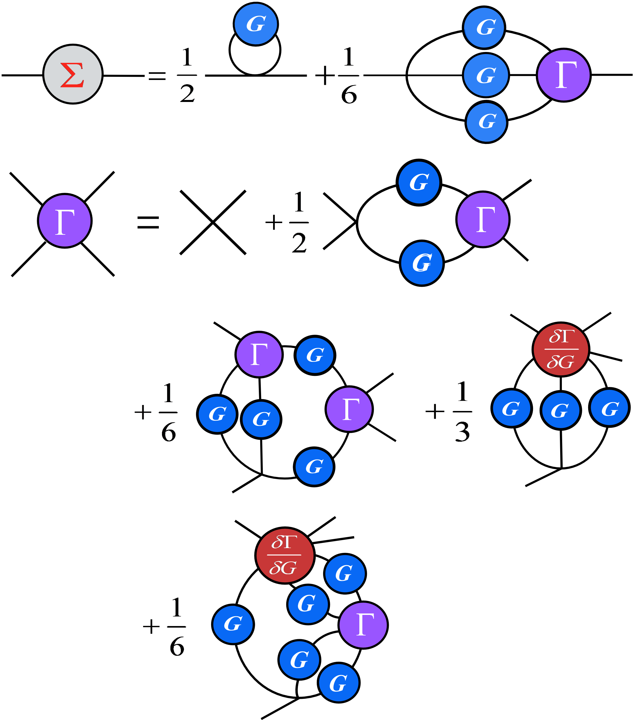
Figure 1: Bold diagrammatic expansions for self energy and 1PI vertex function in $\phi^{4}$ theory. All diagrams on the right hand sides are individually 1PI and expressed in terms of exact propagators.

By differentiating the 1PI vertex function, Eq. (2), with respect to the full propagator, $\bm{G}$, we find series expansions in terms of bold correlation functions for self energy and vertex function, in a recursive way. In particular for the first derivative, we have

$$\frac{\delta\bm{\Gamma}_{b,1234}}{\delta\bm{G}_{b,\alpha\beta}} = -\frac{1}{2}V_{b,12\alpha 6}\bm{G}_{b,68}\bm{\Gamma}_{b,8\beta 34}\;+\alpha\longleftrightarrow\beta+\cdots\;,$$

where dots stand for higher order terms ( higher order in terms of the number of bold propagators). We find that approximating the derivative term by the first term is sufficient for finding the fixed point.

In order to study the behavior of the renormalized coupling constant, we translate the Schwinger-Dyson equations into equations for renormalized correlation functions and impose renormalization conditions

$$\bm{\Gamma}_{r}^{(2)}\,(p^{2}=0) =m^{2}$$ (5)

$$\frac{\partial}{\partial p^{2}}\bm{\Gamma}_{r}^{(2)}\,(p^{2})|_{p^{2}=0} =1$$ (6)

$$\bm{\Gamma}_{r}^{(4)}(0,0,0,0) =m^{4-d}\,g_{r}\;.$$ (7)

The renormalized proper 2-point function which satisfies (5) and (6) can be written as

$$\bm{\Gamma}_{r}^{(2)}(p^{2})\hskip 2.84526pt\equiv\bm{G}^{-1}_{r}(p^{2})=\hskip 2.84526ptZ\,\left(\,p^{2}+\mathbf{Y}(p^{2})\,\right)+m^{2}\;,$$ (8)

where $\mathbf{Y}(p^{2})=\bm{\Sigma}_{b}(p^{2}=0)-\bm{\Sigma}_{b}(p^{2})$ and the field renormalization constant is given by

$$Z=\frac{1}{1+\frac{\partial\mathbf{Y}(p^{2})}{\partial p^{2}}|_{p^{2}=0}}\;.$$ (9)

Using Eq. (Bold Diagrammatic Monte Carlo Study of $\phi^{4}$ Theory) one may rewrite $\mathbf{Y}(p^{2})$ in terms of renormalized quantities as

$$\mathbf{Y}(p^{2})=\frac{g_{0}Z}{6}\int\frac{d^{3}k}{(2\pi)^{3}}\frac{d^{3}q}{(2\pi)^{3}}\bm{G}_{r}(k)\bm{G}_{r}(q)$$ (10)

$$\times\bigg{[}\bm{G}_{r}(Q)\bm{\Gamma}_{r}^{(4)}(0,\overrightarrow{k},\overrightarrow{q},\overrightarrow{Q})-\bm{G}_{r}(Q)\bm{\Gamma}_{r}^{(4)}(\overrightarrow{p},\overrightarrow{k},\overrightarrow{q},\overrightarrow{Q})\bigg{]},$$

where in each term the momentum $\overrightarrow{Q}$ is determined by the conservation of momenta that appear in the vertex function argument. The $\phi^{4}$ theory in 3 dimensions is super-renormalizable and has only three superficially divergent diagrams, all eliminated by the mass counter term. In addition $\mathbf{Y}(p^{2})$ is finite in any order of perturbation. Furthermore all vertex diagrams are superficially finite and we find that it is useful to work with the bare form of the schwinger-Dyson equation (2) in this case, however we have to replace bare two-point functions with the renormalized ones.

Our strategy for computing the renormalized coupling constant corresponding to a given bare coupling is to solve coupled Schwinger-Dyson equations (2) and (10) by means of general BDMC rules, starting with the tree level approximation for correlation functions. After reaching convergence, renormalized coupling constant can be read off from (7) by recalling that $\bm{\Gamma}_{r}^{(4)}=Z^{2}\bm{\Gamma}_{b}^{(4)}$.

In order to increase the efficiency of the algorithm, inspired by the idea of worm algorithm worm and following svis , instead of sampling the $\mathbf{Y}(p)$ and $\bm{\Gamma}_{b}^{(4)}$ directly, we introduce two auxiliary normalization constant terms and sample the following quantities

$$I_{2} = \alpha_{2}+\int\mathbf{Y}(p^{2})\,\Omega(p)^{2}\;dp$$ (11)

$$I_{4} = \alpha_{4}+\int\bm{\Gamma}^{(4)}_{b}(p_{1},p_{2},p_{3},\chi_{12},\chi_{13},\chi_{23})\,d\mathbf{X}$$ (12)

with $d\mathbf{X}=dp_{1}\,dp_{2}\,dp_{3}d\chi_{12}\,d\chi_{13}\,d\chi_{23}$ where $\chi_{ij}$ is cosine of the angle between $\overrightarrow{p_{i}}$ and $\overrightarrow{p_{j}}$, and $\Omega(p)$ is the normalized probability density that we use to generate new momenta in Monte Carlo updates. We skip the details of Monte Carlo procedure and report the results here.

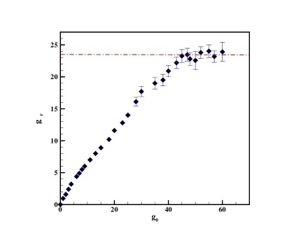
Figure 2: Result of Bold diagrammatic Monte carlo simulation for dimensionless renormalized coupling constant, $g_{r}$, as a function of bare coupling. The asymptotic behavior of renormalized coupling is in agreement with the existence of an IR fixed point.

Fig. 2 depicts the renormalized coupling constant as a function of the bare coupling. As is evident from this plot, $g_{r}$ tends to an asymptotic value in accordance with the renormalization group prediction. Also the value of the fixed point, $\tilde{g}_{r}^{*}=\frac{3}{16\pi}\,g_{r}^{*}=1.40\pm 0.05$, agrees, within error, with the high temperature series expansion and resummed $\epsilon$-expansion zinn ; kl . It is worth noticing that Fig. 2 provides a non-perturbative calculation of $\phi^{4}$ theory based on summing up Feynman diagrams. This plot interpolates between weak and strong coupling regimes and indeed it is not possible to produce such a result by using just perturabtive methods or RG techniques.

It is also interesting to calculate critical exponents by using the BDMC method. Since critical exponents are related to the scaling behavior of composite operators, we construct a new set of Schwinger-Dyson equations for diagrammatic expansion of composite operators in terms of bold correlators. For example the critical exponent $\nu$, which controls the growth of correlation length near the phase transition, is related to the IR behavior of the composite operator with one $\phi^{2}$ insertion, $\bm{\Gamma}^{(1,2)}$. It is straightforward to derive coupled equations for $\bm{\Gamma}^{(1,2)}$ and $\bm{\Gamma}^{(1,4)}$ form (Bold Diagrammatic Monte Carlo Study of $\phi^{4}$ Theory) and (2) by using the mass derivative trick for generating correlation functions with $\phi^{2}$ insertions

$$\bm{\Gamma}^{(1,2)}_{b}(0,p) = 1-\frac{\partial}{\partial m^{2}}\bm{\Sigma}_{b}(p)$$

$$\bm{\Gamma}^{(1,4)}_{b}(0,p) = \frac{\partial}{\partial m^{2}}\bm{\Gamma}^{(4)}_{b}(p)\;.$$

Turning on BDMC machinery it is straightforward to solve this new set of equations in a similar way discussed for (Bold Diagrammatic Monte Carlo Study of $\phi^{4}$ Theory) and (2). We postpone the numerical implementation to future works.

Conclusions and outlook. In summary we described a non-perturbative simulation of a relativistic QFT, $\phi^{4}$ theory in 3-dimensions, based on sampling bold Feynman diagrams. We used a set of coupled Schwinger-Dyson equations to expand physical quantities in terms of exact correlation functions. The systematic method of deriving such bold expansions in quantum field theories was proposed in klei and used to construct connected Feynman diagrams and to calculate their corresponding weights in $\phi^{4}$ theory Pelster:2003rc and quantum electrodynamics Pelster:2001cc . It is based on this fact that a complete knowledge of vacuum energy implies the knowledge of all scattering amplitudes, “ vacuum is the world” js .

In addition, in renormalizable QFT’s it is always possible to formulate such Schwinger-Dyson equations in terms of renormalized correlation functions and finite integrals. Combining with BDMC technique to sampling unknown functions in terms of them, this offers a universal scheme for non-perturbative calculations in QFT’s.

Applying this approach to non-Abelian gauge theories in under progress, however, one may need more complicated resummation methods to recover the correct physical values from truncated bold expansions. In the case of $\phi^{4}$ theory, interestingly, we observed that without using any resummation technique, truncating the series at lowest order, leads to convergent results.

One way to reducing systematic errors produced by the truncation of bold series is introducing a complete basis of functions and expanding correlation functions in terms of them, $\bm{G}_{12}=\sum_{n,m}\;c_{n,m}\,\psi_{n,1}\,\psi_{m,2}$. By considering $\bm{\Gamma}^{(4)}$ as a function of $c_{n,m}$ coefficients the functional derivative term takes the following form

$$\frac{\delta\bm{\Gamma}_{1234}^{(4)}}{\delta\bm{G}_{56}}=\sum_{n,m}\,\frac{\partial\bm{\Gamma}_{8234}}{\partial c_{n,m}}\;\psi_{n,5}\,\psi_{m,6}\;.$$ (13)

Performing a Monte Carlo process in space of $c_{n,m}$ coefficients to sample the derivative term, increases the accuracy of the algorithm drastically.

The author would like to thank N. Abbasi, A. Fahim, A. Akhavan, D. Allahbakhsi, R.Mozafari, H. Seyedi and A.A Varshovi for discussions. I would also like to thank M. Alishahiha and A.E. Mosaffa for helpful discussions and for carefully reading and commenting on the manuscript.

References

- (1) N.V. Prokof’ev, B.V. Svistunov, and I.S. Tupitsyn, JETP 87, 310 (1998).
- (2) N.V. Prokof’ev and B.V. Svistunov, Phys. Rev. Lett. 81, 2514 (1998).
- (3) Van Houcke, K., Kozik, E., Prokofev, N. and Svistunov, B. in Computer Simulation Studies in Condensed Matter Physics XXI (eds Landau, D. P., Lewis, S. P. and Schuttler, H. B.) (Springer, 2008).
- (4) E. Burovski, N. Prokof’ev, B. Svistunov, and M. Troyer, Fermi-Hubbard model at Unitarity,. New J. Phys. 8, 153 (2006).
- (5) P. V. Buividovich, Nucl. Phys. B 853, 688 (2011).
- (6) Prokofev, N. and Svistunov, B. Bold diagrammatic Monte Carlo technique: When the sign problem is welcome. Phys. Rev. Lett. 99, 250201 (2007).
- (7) K.Van Houcke, et al. Feynman diagrams versus Fermi-gas Feynman emulator, Nat. Phys. 8, 366 (2012).
- (8) Wilson, K.G. and Fisher, M.E. Phys.Rev.Lett. 28, 240 (1972).
- (9) Parisi G. J. Stat. Phys., 1980, vol. 23,. No 1, p. 49-82.
- (10) J. Zinn-Justin, Quantum Field Theory and Critical Phenomena, 4th ed. 1054p., Oxford University Press (2002).
- (11) Hagen Kleinert V. Schulte-Frohlinde Critical Properties of Phi4-Theories pp. 1-489, World Scientific, Singapore 2001.
- (12) A. Pelster and K. Glaum, Physica A 335, 455 (2004).
- (13) N.V. Prokof’ev and B.V. Svistunov,Phys. Rev. Lett. 87, 160601 (2001).
-
(14)
B.V. Svistunov,
wiki.phys.ethz.ch/quantumsimulations/
_media/svistunov2.pdf - (15) H. Kleinert, Fortschr. Phys. 30, 187 and 351 (1982).
- (16) A. Pelster, H. Kleinert and M. Bachmann, Annals Phys. 297, 363 (2002).
- (17) J. Schwinger, Particles, Sources, and Fields, Vols. I and II (Addison-Wesley, Reading, 1973).