Probability-Matching Predictors for Extreme Extremes

Abstract

A location- and scale-invariant predictor is constructed which exhibits good probability matching for extreme predictions outside the span of data drawn from a variety of (stationary) general distributions. It is constructed via the three-parameter $\{\mu,\sigma,\xi\}$ Generalized Pareto Distribution (GPD). The predictor is designed to provide matching probability exactly for the GPD in both the extreme heavy-tailed limit $\xi\rightarrow\infty$ and the extreme bounded-tail limit $\xi\rightarrow-\infty$, whilst giving a good approximation to probability matching at all intermediate values of the tail parameter $\xi$. The predictor is valid even for small sample sizes $N$, even as small as $N=3$.

The main purpose of this paper is to present the somewhat lengthy derivations which draw heavily on the theory of hypergeometric functions, particularly the Lauricella functions. Whilst the construction is inspired by the Bayesian approach to the prediction problem, it considers the case of vague prior information about both parameters and model, and all derivations are undertaken using sampling theory.

1 Introduction

This paper presents a novel approach to extrapolation beyond the span of historical data, one of the basic problems of inference. The notion of say the “1 in 10,000 year event” exists in common parlance, even though the philosophical interpretation of the phrase differs in detail between Bayesian and non-Bayesian schools. Often the analyst has only a limited set of historical data, say of the order of 100 years, but is asked to make predictions regarding possible future events (at say the “1 in 10,000 year level”) which are substantially greater than historical experience. The paper concerns the issue of whether there are rational methods for tackling this philosophically-fraught problem, and the method developed here - whilst only in its preliminary stages of development - is presented as a potential candidate which may be worthy of further exploration. Although the following theory is created around properties of the Generalised Pareto Distribution (GPD) and its tail parameter $\xi$, the final predictor created is non-parametric. Its usefulness or otherwise remains to be determined, but nevertheless it has some remarkable properties.

We consider here only the univariate case, with the data consisting of a set of $N$ discrete real-valued “events” $\bm{x}$ drawn from a stationary distribution $F_{\bm{\theta}}$ with unknown parameters $\bm{\theta}$. The approach presented focuses directly on prediction rather than estimation, and the key concept is that of probability matching. The phrase has been given precise definitions elsewhere (e.g. Datta and Mukerjee (2004); Sweeting (2008)) and refers to cases when coverage probabilities of Bayesian and frequentist approaches coincide. The use of the phrase here is similar, but for the predictors in question it is not clear that a Bayesian prior exists, thus the phrase will be applied here directly to the predictor. Its usage here is an attempt to formalise the loose notion that a prediction of the “1 in T” level event $x_{T}$ should actually deliver what it appears to promise: that the probability that the next event $x_{next}$ will exceed $x_{T}$ is indeed $1/T$. Of course, this loose notion needs to be formalised, particularly since Bayesians will disagree with non-Bayesians about even what is meant by “probability”.

In the frequentist approach, the analyst typically uses the data $\bm{x}$ to construct a point estimate $\hat{\bm{\theta}}$ of the actual unknown parameters $\bm{\theta}_{0}$ of the assumed model, and then uses the tail of the family member $F_{\hat{\bm{\theta}}}$ to select the value $\hat{x}_{T}$, via $F_{\hat{\bm{\theta}}}(\hat{x}_{T})=1-1/T$. Thus $\hat{x}_{T}$ is an estimate of the actual (but unknown) value $x_{T}$ that has an exceedance probability $1/T$ for the actual (but unknown) distribution $F_{\bm{\theta}_{0}}$ from which the data was drawn. Confidence intervals may then be constructed around that estimate $\hat{x}_{T}$ at some chosen confidence level, and a designer or decision maker may perhaps choose to use the upper confidence level as the basis for the “1-in-T level” event. Note that there is thus a mixture of notions of probability here: the designer may aim for the 1 in 10,000 event but may only have a 95% confidence in the result.

In the Bayesian approach, the analyst combines the data with prior knowledge about the parameters to construct the posterior distribution on the parameters, this being a representation of the analyst’s updated beliefs about the parameters of the model. Rather than simply choosing the single family member with the parameter value set to the point estimate which has the greatest posterior belief value, the Bayesian takes account of uncertainty in knowledge of the parameters by constructing the predictive distribution, this being the analyst’s updated beliefs about the possible value of the next data element $x_{next}$. The predictive distribution is, loosely speaking, the integral of all probabilities of all possibilities. The Bayesian candidate for the “1 in T” level is that value $x_{T}$ above which lies a fraction $1/T$ of the analyst’s beliefs about $x_{next}$. That is, extreme value predictions at some given return level are set at the value above which the tail integral of the predictive distribution equals the desired exceedance probability (see Coles and Tawn (2005), for example). Despite the appealing rationality of the procedure, it is not without difficulties. For predictions well outside the span of the data, the tails of the predictive distribution may be strongly influenced by the prior beliefs about model parameters, and this can be problematic when prior knowledge - particularly regarding the tail parameters - is vague. Moreover, standard numerical integration techniques such as MCMC can require excessively long run times to explore the tail regions outside the data sufficiently often for the analyst to be confident that the numerically-generated distributions have converged sufficiently.

The problem of predicting the “1 in T” level event has solutions in various restricted cases. For example, the Bayesian predictor $x_{T}$ based on some proper prior $\Pi(\bm{\xi})$ matches probability at the target level $T$ in the sampling sense, sampling parameters $\bm{\xi}_{i}$ from $\Pi(\bm{\xi})$ and then sampling the data (and $x_{next}$) from the chosen distribution $F_{\bm{\xi}_{i}}$. The two parameter ($\mu,\ \sigma$) location-scale families provide other ready examples. For example, if the data $\bm{x}$ is sampled from some unknown member of some known family of location-scale distributions $F(y)$ with $y=(x-\mu)/\sigma$, then any statistic of the form $s_{T}=s_{LS}+\beta s_{S}$ (where $s_{LS}$ is location-scale invariant and $s_{S}$ is scale invariant) is a probability-matching predictor at some level $T=T(\beta)$. Specifically, the predictor $x_{T}$ that arises from the Bayesian approach using the (improper) $1/\sigma$ prior matches probability at the designed-for level $T$ (see McRobie (2004)). (Priors using other powers of $\sigma$ give probability performance which is location- and scale-invariant, but not at the designed-for level).

Although the $1/\sigma$ predictor has the pleasing property of delivering the required $T$ level performance no matter what the parameter values actually are, one obvious short-coming that limits its usefulness is the requirement for complete prior knowledge of the model. That is, the functional form of the two-parameter family of distributions $F$ must be known a priori. The compass of the procedure would thus be somewhat expanded if it could be extended to cover three-parameter location-scale-shape families of the form $F(y)$ with $y=\left((x-\mu)/\sigma\right)^{-1/\xi}$. Since both the Generalized Pareto and Generalised Extreme Value distributions (GPD, GEV) can be expressed in this form, the possibility may then exist that the machinery of Extreme Value Theory (e.g. Embrechts et al. (1999)) could also be invoked in order to apply the predictor to data sets drawn from more general distributions. Loosely speaking, since - under suitable conditions - the upper order statistics of samples drawn from more general distributions have the GPD as their limiting distribution, then a probability-matching predictor for the GPD may have wider application.

The question thus arises as to whether probability-matching predictors can be constructed in the general three-parameter ($\mu$, $\sigma$, $\xi$) case. If so, there are the further questions as to whether there is a corresponding prior, and what form that prior might be.

This paper endeavours to construct a probability-matching predictor for the three-parameter GPD. By taking a sampling - rather than a Bayesian - approach, predictors are constructed such that probability matching is exact in the both the extreme heavy-tailed ($\xi\rightarrow\infty$) and extreme bounded-tail ($\xi\rightarrow-\infty$)) limits. At finite values of $\xi$, probability is only approximately matched, but the degree of approximation is very good. Moreover the predictor applies to samples as small as $N=3$, and works remarkably well for predictions which lie far outside the span of the data. Finally, when applied to small data sets sampled from non-GPD distributions, out-of-sample predictions match probability to a remarkably close approximation.

2 Sampling Distributions of the Normalised Data

Suppose $N$ data points $\bm{x}=\{x_{1},\ldots,x_{N}\}$ are sampled from a Generalised Pareto Distribution (GPD) with distribution function

$$F(x)=1-{\left(1+\xi\frac{(x-\mu)}{\sigma}\right)}^{-1/\xi}$$ (1)

with unknown parameters $(\mu,\sigma,\xi)$. Let the ordered data be $\bm{X}=\mathrm{sort}(\bm{x})$, such that $X_{1}\leq X_{2}\leq\ldots\leq X_{N}$. (Note that the indexing of the ordered data is from the lowest order statistic, and that this is in the opposite direction to that adopted in McRobie (2013b) and McRobie (2013a)).

The aim is to construct a predictor $x_{T}(\bm{X})$ such that, for any chosen return level $T$, there is a probability $1/T$ that the next data point $x_{next}$ will exceed $x_{T}$. That is, we desire

$$P(x_{next}>x_{T})=\frac{1}{T}$$ (2)

irrespective of the values of the parameters $(\mu,\sigma,\xi)$ of the distribution from which the data was sampled.

We first normalise the data to lie within the unit interval via the statistics $\bm{t}=\{t_{1},t_{2},\ldots,t_{N-2}\}$ with

$$t_{j}\equiv\frac{X_{j+1}-X_{1}}{X_{N}-X_{1}}\qquad j=1,\ldots(N-2)$$ (3)

Clearly, $0\leq t_{1}\leq t_{2}\leq\ldots\leq t_{N-2}\leq 1$.

The normalised data is location- and scale-independent, in that $\bm{t}(\bm{X})=\bm{t}(a\bm{X}+b\bm{1})$ for any $a>0$ and any $b$. The normalisation is simply a linear mapping of the data onto the interval $[0,1]$, the data minimum $X_{1}$ mapping to zero and the data maximum $X_{N}$ mapping to 1.

We are interested in extrapolating to possible large future extremes which lie outside the span of previous data. The next data point $x_{next}$ might not exceed the data maximum $X_{N}$, but we shall be most interested in those cases when it does. We shall thus denote the next data point $x_{next}$ as $x_{N+1}$. We will likewise focus on constructing predictions $x_{T}$ in that region beyond the data maximum.

The next data point $x_{next}=x_{N+1}$ and the prediction $x_{T}$ may be normalised via

$$s\equiv\frac{x_{N+1}-X_{1}}{X_{N}-X_{1}}\ \ \ \ \mathrm{and}\ \ \ \ s_{T}(\bm{t})\equiv\frac{x_{T}(\bm{X})-X_{1}}{X_{N}-X_{1}}$$ (4)

Given the parameters $\{\mu,\sigma,\xi\}$, the sampling density $p(\mathbf{t}|\mu,\sigma,\xi)$ of the statistics $\mathbf{t}$ may, via the elementary integrations of Appendix 1, be expressed in terms of a Lauricella function $F_{D}$. Since the statistics $\bm{t}$ are location- and scale-independent, the sampling density retains a parameter dependence only through the shape parameter $\xi$.

Writing $N_{1}=N-1$ for brevity, then in the region of the heavy-tailed ($\xi>0$) GPDs, writing $\alpha\equiv\xi^{-1}>0$, we obtain from Appendix 1 that

$$p(\bm{t}|\xi,(\xi>0)) = N_{1}!\ \alpha^{N_{1}}\ \ \Gamma\left[\begin{array}[]{c}N_{1},\ N_{1}\alpha\\ N_{1}(1+\alpha)\end{array}\right]\ F_{D}^{(N-2)}\left(N_{1},\bm{1}+\bm{\alpha};N_{1}(1+\alpha);\bm{\tau}\right)$$ (7)

where $\bm{1}$ is a vector of $(N-2)$ ones, $\bm{\alpha}\equiv\alpha\bm{1}$ and $\bm{\tau}\equiv\bm{1}-\bm{t}$.

For the bounded-tail ($\xi<0$) GPDs, writing $\beta\equiv-\xi^{-1}>0$, we similarly obtain

$$p(\bm{t}|\xi,(\xi<0)) = N_{1}!\ \beta^{N_{1}}\ \ \Gamma\left[\begin{array}[]{c}N_{1},\ N_{1}\beta\\ N_{1}+\beta\end{array}\right]\ F_{D}^{(N-2)}\left(N_{1},\bm{1}-\bm{\beta},N_{1}+\beta;\bm{t}\right)$$ (10)

with $\bm{\beta}\equiv\beta\bm{1}$.

3 The Problem Statement

Since all dependence on the location and scale parameters has been removed by the normalisation, the only parameter of remaining interest is the tail parameter $\xi$.

Given the parameters $\xi$, the probability that the next (normalised) event $s$ will exceed some given function $s_{T}(\bm{t})$ of any data $\bm{t}$ is given by

$$P(s>s_{T}(\bm{t})|\xi)=\int\bm{G}(s_{T}(\bm{t})|\xi)\ p(\bm{t}|\xi)\ d\bm{t}$$ (11)

where $d\bm{t}=dt_{1}dt_{2}\ldots dt_{N-2}$ and the integral is over all admissible normalised data $\bm{t}$, and the integrand is defined via

$$G(s_{T}(\bm{t})|\xi)p(\bm{t}|\xi)\equiv\int_{s_{T}(\bm{t})}^{\infty}\ p(s,\bm{t}|\xi)\ ds$$ (12)

In the heavy-tailed region ($\alpha\equiv 1/\xi>0$), for the case of interest where $s_{T}>1$, the elementary integrations of Appendix 2 reveal the integrand of equation 11 to be

$$\bm{G}(s_{T}(\bm{t})|\xi)\ p(\bm{t}|\xi) = \frac{N!}{N+1}\ \alpha^{N_{1}}\ \ \Gamma\left[\begin{array}[]{c}N_{1},\ N\alpha\\ N_{1}+N\alpha\end{array}\right]\frac{t_{1}^{N_{1}\alpha-1}}{\left(t_{2}\ldots t_{N-2}\right)^{1+\alpha}s_{T}^{\alpha}}\ldots$$ (16)

$$\hskip 28.45274pt\times\ F_{D}^{(N-1)}\left(N\alpha,\bm{1}+\bm{\alpha},\alpha;N_{1}+N\alpha;\bm{\kappa}\right)$$

where the $j$-th element of $\bm{\kappa}$ is $\kappa_{j}=1-t_{1}/t_{j}$ for $j=2,\ldots,N$, the $t_{j}$ notation being extended here to include the two further points $t_{N-1}=1$ and $t_{N}=s_{T}$.

For the bounded-tail region ($\beta\equiv-1/\xi>0$), the corresponding integrand is

$$\bm{G}(s_{T}(\bm{t})|\xi)\ p(\bm{t}|\xi) = \frac{N!}{N+1}\ \beta^{N_{1}}\ \ \Gamma\left[\begin{array}[]{c}N_{1},\ 1+\beta\\ N+\beta\end{array}\right]\ \frac{1}{s_{T}^{N_{1}}}\ldots$$ (20)

$$\hskip 19.91692pt\times\ F_{D}^{(N-1)}\left(N_{1},\bm{1}-\bm{\beta},1-\beta;N+\beta;\frac{\bm{t}}{s_{T}},\frac{1}{s_{T}}\right)$$

The problem statement is thus: for any $T>N+1$, find a function $s_{T}(\bm{t})$ over the normalised data space which, when substituted into Eqns 11-20, is such that $P(s>s_{T}(\bm{t})|\xi)=1/T$ for any $\xi$.

4 The Heavy-Tailed Limit $\xi\rightarrow\infty$

We consider first those predictors which guarantee to match probability at the $1/T$ level for those distributions in the limit of extremely heavy tails $\xi\rightarrow\infty$. For large $\xi$ (i.e. small $\alpha$), the Lauricella function in Eqn. (16) approaches unity due to the argument $N\alpha$ in its first slot. The conditional exceedance integrand of Eqn. (16) thus simplifies to

$$\bm{G}(s_{T}(\bm{t})|\xi)p(\bm{t}|\xi)\approx\frac{N!}{N+1}\ \alpha^{N_{1}}\ \Gamma\left[\begin{array}[]{c}N_{1},\ N\alpha\\ N_{1}+N\alpha\end{array}\right]\ \frac{t_{1}^{N_{1}\alpha-1}}{\left(t_{2}\ldots t_{N-2}\right)^{1+\alpha}s_{T}^{\alpha}}$$ (21)

Since any function of the statistics $\bm{t}$ is a predictor, there is an almost limitless variety to the possible functional forms that our predictor $s_{T}(\bm{t})$ might take.

To progress, we consider predictors taking a power law form:

$$s_{T}=\prod_{j=1}^{N-2}\ {t_{j}}^{-\lambda_{j}}$$ (22)

Integrating (21) over the domain $0\leq t_{1}\leq\ldots\leq t_{N-2}\leq 1$ and setting the result equal to the desired exceedance probability $1/T$ leads to the constraint

$$\prod_{j=1}^{N-2}\left(1+\frac{\gamma_{j}}{N-j}\right)=\frac{T}{N+1}\ \ \mathrm{where}\ \ \gamma_{j}=\sum_{k=1}^{j}\lambda_{k}$$ (23)

For $N=3$, this constraint requires

$$\lambda_{1}=\gamma_{1}=2\left(\frac{T}{4}-1\right)$$ (24)

For larger samples and for a given $T$, the constraint equation (23) defines an $(N-3)$-dimensional space of possible exponents for our power-law predictor. One obvious solution sets each term in the left-hand product of equation (23) equal to the same value, $(T/(N+1))^{1/(N-2)}$, giving

$$\gamma_{j}=(N-j)\left[\left(\frac{T}{N+1}\right)^{\frac{1}{N-2}}-1\right]$$ (25)

An alternative choice is one that gives predictions that are in some sense small, and the expected value of $\log(s_{T})$ can be minimised by choosing

$$\gamma_{j}=(N-j-1)K-(N-j)\ \ \mathrm{with}\ \ K=\left[\frac{N-1}{N+1}\ T\right]^{\frac{1}{N-2}}$$ (26)

For simplicity, we might instead choose to make all the $\lambda_{j}$ the same ($=\lambda$). For any sample size $N$ and any desired return level $T$, the exponents of the power-law predictor can be obtained numerically (e.g. by a simple bisection method) to determine that value of $\lambda$ which satisfies the constraint equation. Values of $\lambda$ so determined are given in Table 1.

Table 1: Exponents $\lambda$ satisfying the heavy-tailed constraint equation 23

$\frac{T}{N+1}$	N=3	N=7	N=15	N=31
2	2	0.1507	0.0354	0.0113
4	6	0.3363	0.0750	0.0233
8	14	0.5615	0.1188	0.0361
16	30	0.8317	0.1672	0.0498
32	62	1.1530	0.2202	0.0642
64	126	1.5325	0.2782	0.0795
128	254	1.9785	0.3412	0.0956
256	510	2.5003	0.4097	0.1125
512	1022	3.1086	0.4838	0.1303
1024	2046	3.8157	0.5638	0.1489
2048	4094	4.6359	0.6501	0.1684
4096	8190	5.5854	0.7430	0.1888

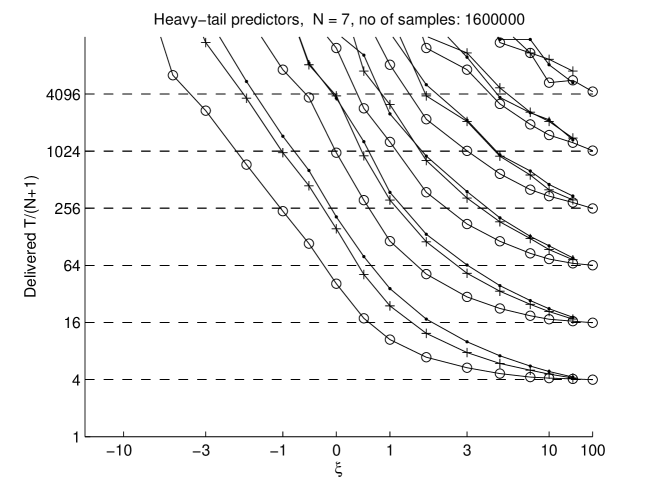
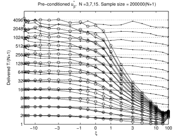
The performance of the above predictors when played against samples drawn from distributions with various shape parameters $\xi$ are shown in Figure 1. All give the desired performance in the extremely heavy-tailed limit (at the right of the diagram), but over-predict elsewhere.

The predictors in this heavy-tailed limit we shall denote by $u_{\alpha}=s_{T}-1$, this being the (scaled) excess of the prediction above the data maximum.

Figure 1: The probability performance of the heavy-tailed predictors. The figure shows the return levels delivered by the predictors of Eqns. 25 (.), 26(+) and with all $\lambda_{j}=\lambda$ (o) for samples of size $N=7$. In each case, predictors were asked to predict at return levels of $T/(N+1)=4,16,64,256,1024\ \text{and}\ 4096$. All three predictors satisfy the heavy-tail constraint equation 23 and the convergent lines at the right-hand side of the figure support the proposition that each matches probability at the target level in the heavy-tailed limit.

5 The Bounded-Tail Limit $\xi\rightarrow-\infty$

In this section a constraint equation is constructed for the exponents of a power law predictor which will deliver exact probability matching in the extreme limit of large negative $\xi$. Such a constraint is somewhat more difficult to find. The derivation in Appendix 3 shows that a predictor can be constructed of the form $s_{T}=1+u_{\beta}$ where

$$u_{\beta}=\tau_{N-2}\ \frac{\bm{\tau}^{P}}{1-\bm{\tau}^{P}}\ \ \mathrm{where}\ \bm{\tau}^{P}\equiv\prod_{j=1}^{N-2}\tau_{j}^{\rho_{j}}$$ (27)

and the exponents $\rho_{j}$ of each $\tau_{j}=1-t_{j}$ must satisfy the constraint

$$\prod_{k=1}^{N-2}\left[\frac{2\eta_{k}}{k+2}+1\right]=\frac{1}{1-\frac{N+1}{T}}\ \mathrm{where}\ \eta_{k}=\sum_{j=N-1-k}^{N-2}\rho_{j}$$ (28)

For $N=3$ there is a single solution

$$\rho_{1}=\eta_{1}=\frac{3}{2\left(\frac{T}{4}-1\right)}=\frac{3}{\lambda_{1}}$$ (29)

which is reciprocally related to the exponent $\lambda_{1}$ of the corresponding extreme heavy-tailed case.

Again, for larger sample sizes and given $T$, the constraint defines an $(N-3)$-dimensional manifold of possible exponents, and various ad hoc schemes can be readily devised that satisfy the constraint. For further progress, we consider only the scheme which sets all exponents $\rho_{j}$ equal to the same value $\rho$ for some given $T$. Since the constraint equation is a polynomial of degree $N-2$ in $\rho$, this can again be solved numerically for $\rho$ at any $T$, for example by using a simple bisection method. Values of $\rho$ for $N=3$, 7, 15 and 31 are given in Table 2.

Table 2: Exponents $\rho$ satisfying the extreme bounded-tail constraint equation 28

$\frac{T}{N+1}$	N=3	N=7	N=15	N=31
2	1.5	0.1326	0.0381	0.0147
4	0.5	0.0527	0.0155	6.0377$\times 10^{-3}$
8	0.2066	0.0241	7.1688$\times 10^{-3}$	2.7948$\times 10^{-3}$
16	0.1	11.544$\times 10^{-3}$	3.4548$\times 10^{-3}$	1.3491$\times 10^{-3}$
32	0.0484	5.6596$\times 10^{-3}$	1.6975$\times 10^{-3}$	0.6633$\times 10^{-3}$
64	0.0238	2.8022$\times 10^{-3}$	0.8414$\times 10^{-3}$	0.3271$\times 10^{-3}$
128	11.809$\times 10^{-3}$	1.3945$\times 10^{-3}$	0.4189$\times 10^{-3}$	0.1638$\times 10^{-3}$
256	5.8796$\times 10^{-3}$	0.6953$\times 10^{-3}$	0.2089$\times 10^{-3}$	0.0817$\times 10^{-3}$
512	2.9337$\times 10^{-3}$	0.3457$\times 10^{-3}$	0.1044$\times 10^{-3}$	0.0408$\times 10^{-3}$
1024	1.4644$\times 10^{-3}$	0.1733$\times 10^{-3}$	0.0521$\times 10^{-3}$	0.0204$\times 10^{-3}$
2048	0.7186$\times 10^{-3}$	0.0866$\times 10^{-3}$	0.0261$\times 10^{-3}$	0.0102$\times 10^{-3}$
4096	0.3662$\times 10^{-3}$	0.0432$\times 10^{-3}$	0.0130$\times 10^{-3}$	0.0050$\times 10^{-3}$

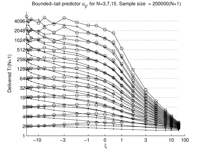
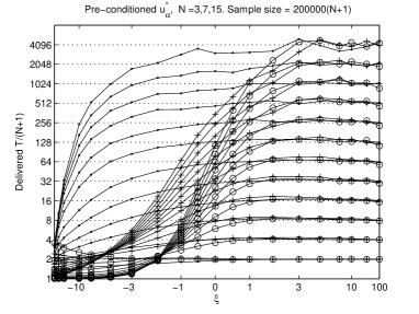
The performance of the resulting predictor is illustrated in Fig. 2 for $N=3$, 7 and 15, showing that $1/T$ exceedance is delivered in the extreme bounded-tail limit $\xi\rightarrow-\infty$, but typically under-predicting for less extreme tail parameters.

Figure 2: The probability performance of the extreme bounded-tail predictor $u_{\beta}$, wherein all exponents $\rho_{j}=\rho$ satisfy the constraint Eqn. 28 derived in Appendix 3. The figure gives the return levels delivered for samples of size $N=3$(.), 7(+) and 15(o), and the convergent lines to the left of the figure suggest that such predictors do indeed match probability in the extreme bounded-tail limit.

6 Predictors at specific intermediate values of $\xi$

We now possess predictors $u_{\alpha}$ and $u_{\beta}$ which match probability in the two extreme limits. Individual predictors can readily be constructed at any specific known $\xi$ between these two limits. For example at the GPDs where $\xi=0$ and $\xi=-1$ (the exponential and the uniform) any number of location- and scale-invariant predictors can be constructed which match probability there, and a simple example is provided by the Bayesian $1/\sigma$ predictors.

For $\xi=0$ (exponential), the $1/\sigma$ Bayesian predictor is

$$s_{T}=(1+\sum_{j=1}^{N-2}t_{j})\ \left[\left(\frac{NT}{N+1}\right)^{1/(N-1)}-1\right]$$ (30)

and for $\xi=-1$ (uniform) it is simply the constant

$$s_{T}=\left(\frac{T}{N+1}\right)^{1/(N-1)}$$ (31)

The performance of these two predictors over a range of shape parameters is illustrated in Fig. 3. It can be seen that they do indeed deliver the required prediction performance at the shape parameter for which they are designed, but the performance deviates rapidly away from the desired level at nearby shape parameters. This illustrates the danger of designers assuming that data is say exponentially distributed and predicting accordingly, for if the data is actually drawn from a nearby GPD the predictions might be extremely optimistic, and the designer should not be so surprised when the design is soon exceeded.

Figure 3: The numerical performance of the $1/\sigma$ Bayes predictors for $\xi=-1$ uniform (left) and $\xi=0$ exponential (right). Both deliver the desired exceedance performance only at the respective shape parameters (along the central vertical in each diagram) that they have been designed for.

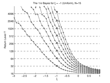
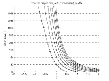
Note that the exponential $1/\sigma$ predictor does not predict the data maximum ($s_{T}=1$) for the return level $T=N+1$. It can even predict values below the data maximum (e.g. for $N=3$, $s_{T=4}=(\sqrt{3}-1)(1+t)$, which can be as low as $s_{T=4}=0.7321$). This differs from the strategy that will be adopted in this paper. Here the aim is to create more general predictors and the decision has thus been made that these should all pass through the only presently known (albeit trivial) example of a universal probability-matching extreme value predictor (namely the data maximum for the $T=N+1$ prediction, corresponding to $s_{T=N+1}=1$).

In the absence of a known non-informative prior on the shape parameter, a number strategies could be adopted for constructing predictors which attempt to match probability across the full range of $\xi$. In this paper, the approach will be to interpolate between the two extreme predictors $u_{\alpha}$ and $u_{\beta}$.

7 Predictions across all shape parameters

The two extreme predictors proposed thus far each define a surface $u(\bm{t})$ above the $(N-2)$-dimensional simplex of all possible normalised data $\bm{t}$. If there is a general predictor which matches probability at all $\xi$, then one might expect its prediction surface $u(\bm{t})$ to approach $u_{\alpha}(\bm{t})$ for small $t_{j}$ and $u_{\beta}(\bm{t})$ for $t_{j}$ near unity, these being the regions where data tends to congregate in the respective extreme limits.

A large number of interpolation schemes were considered but for brevity, only one such scheme is presented here.

7.1 An interpolated predictor

First we pre-condition the two extreme predictors $u_{\alpha}$ and $u_{\beta}$ such that they give better probability matching over wider ranges of $\xi$ than the extreme limits for which they have been designed, and then we interpolate.

Pre-multiplying $u_{\alpha}$ and $u_{\beta}$ by some power of the geometric means $\tilde{\tau}$, $\tilde{t}$ of $\bm{\tau}$, $\bm{t}$ respectively, can improve their performance over wider ranges of $\xi$ whilst matching probability in their respective limits. That is, moderated predictors can be constructed of the form

$$u_{\alpha}^{*} = \tilde{\tau}^{A}u_{\alpha}$$ (32)

$$u_{\beta}^{*} = \tilde{t}^{B}u_{\beta}$$ (33)

where the exponents $A$ and $B$ are chosen by numerical experiments such that $u_{\alpha}^{*}$ and $u_{\beta}^{*}$ give reasonable probability matching over most of their respective $\xi>0$ and $\xi<0$ ranges (see Fig. 4). Candidate values for $A$ and $B$ determined on the basis of such numerical experiments are shown in Table 3.

Figure 4: The probability performance of the pre-conditioned predictors $u_{\beta}^{*}$ and $u_{\alpha}^{*}$ for samples of size $N=3$ (.), 7 (+) and 15 (o), showing reasonable probability matching over large areas of the respective $\xi<0$ or $\xi>0$ regions.

Table 3: Empirically-determined exponents $A$ and $B$ of the moderated predictors of Eqn. 33 used to construct Figs. 4 and 5

	A				B
$\frac{T}{N+1}$	N=3	N=7	N=15	N=31	N=3	N=7	N=15	N=31
2	4	2.2	2.5	3	0	0.45	0.7	0.75
4	2	2.38	3.0	3.5	-2	0.3	0.5	0.55
8	1.5	2.57	3.5	4.2	-6	0.2	0.3	0.4
16	1.25	2.78	4.0	5.05	-14	0.1	0.2	0.3
32	1	3.02	4.5	6	-30	0.05	0.1	0.2
64	0.8	3.3	5.0	7	-62	0.02	0.05	0.1
128	0.6	3.6	5.5	8	-126	0.01	0.25	0.05
256	0.55	3.9	6.0	9	-254	0.005	0.0125	0.025
512	0.5	4.2	6.5	10	-510	0.0025	0.0063	0.0125
1024	0.5	4.5	7.0	11	-1022	0.0012	0.0031	0.0063
2048	0.5	4.8	7.5	12	-2046	0.0006	0.0016	0.0031
4096	0.5	5.1	8.0	13	-4094	0.0003	0.0008	0.0016

A combined predictor can then be constructed via simple linear interpolation between the two moderated prediction surfaces. The interpolation chosen is based on the “elemental estimators” of McRobie (2013b). These are a family of simple location- and scale-invariant estimators based on log-spacings of the data, and they were shown to be absolutely unbiased estimators of the shape parameter $\xi$ of the GPD. The specific estimator $\hat{\xi}$ used here is the one which gives equal weight to each elemental estimator.

The interpolation functions are

$$f_{1}=\frac{e^{\hat{\xi}}}{1+e^{\hat{\xi}}}\ \ \ \mathrm{and}\ \ f_{2}=1-f_{1}=\frac{e^{-\hat{\xi}}}{1+e^{-\hat{\xi}}}$$ (34)

The resulting total predictor $u_{T}$ is

$$u_{T}=f_{1}u_{\alpha}^{*}+f_{2}u_{\beta}^{*}$$ (35)

All elements of this predictor have some analytical justification except for the two numerically-determined pre-conditioning exponents $A$ and $B$. Prediction at the return level $T$ from any data sample of size $N$ can thus be computed by the above formula, and requires knowledge of only two numbers, $A$ and $B$, determined by numerical experiments.

Figure 5: The probability performance of the interpolated predictor of Eqn. 35 for samples of size $N=3$, 7, 15 and 31. Good probability matching is obtained for extrapolation factors $T/(N+1)$ of up to 100 or more.

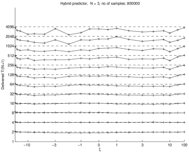
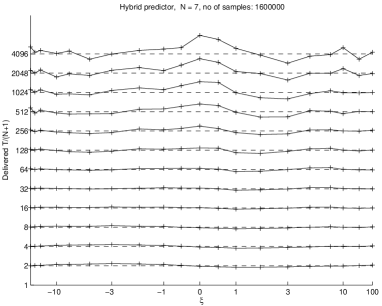
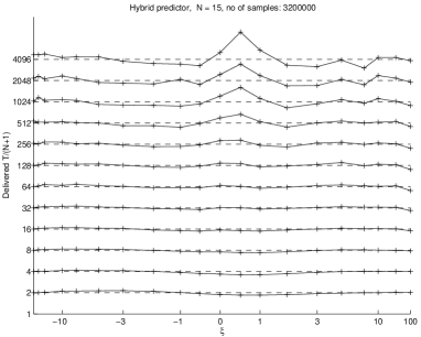
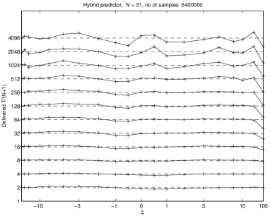
The performance of the interpolated predictor is shown in Fig. 5 for samples of size $N=3$, 7, 15 and 31. It can be seen that probability is matched to a good approximation in all cases across the full range of $\xi$, even for extrapolations to return levels far beyond the span of the data. The probability matching is almost exact in the lower half of each figure, which corresponds to prediction factors $T/(N+1)$ of up to 100 - i.e. a predictor with a return level up to $T\approx 300$ can be constructed for a sample of size 3, and up to $T\approx 3000$ for a sample of size 31. Such large extrapolations beyond the data are often demanded in engineering: design for the 10,000 year event often being required from around 100 years of historical data.

Figure 6: Typical extrapolation by the interpolated predictor. The data, shown by dots in the bottom left corner, is a random sample of size $N=15$ from an exponential distribution (the GPD with $\xi=0$). The predictions at various levels of $T$ are shown as the solid line (+) rising to the right. The actual quantiles for the sampled distribution are shown by the dashed line and the $1/\sigma$ Bayes predictions (knowing that $\xi=0$) are shown as circles.

A typical extrapolation by the interpolated predictor is illustrated in Fig. 6. Extrapolation is from a sample of size $N=15$ drawn from a GPD with $\xi=0$ (i.e. an exponential distribution). The data (dots, bottom left) is plotted against the empirical return levels (both logarithmic), and the predictions are plotted likewise against the corresponding return level aimed for. The actual quantiles are also plotted (dashed), together with the $1/\sigma$ Bayes predictions (knowing that the data is drawn from an exponential). The predictions of the interpolated predictor typically exceed the actual quantile by a considerable margin, reflecting the uncertainty in the actual value of $\xi$. Loosely speaking, although the data may suggest that there is a high likelihood that the underlying distribution is indeed exponential, the interpolated predictor recognises that there remains an appreciable chance that the data may have been drawn from a heavy-tailed GPD with a value of $\xi>0$.

This inherent bias towards larger predictions must not be confused with risk aversion. The actual quantiles (dashed lines) can only be drawn here because the underlying parameters are known. In practice the parameters will be unknown, and the prediction algorithm has been designed to allow for the possibility that the data may have come from any GPD, including those with heavier tails.

8 Application to other distributions

The interpolated predictor $u_{T}$ is now applied to samples drawn from a variety of distributions outside the GPD family. The results are shown in Fig. 7, where the delivered return interval is plotted against that designed for.

The $N=7$ version of $u_{T}$ was used. This is applicable to any sample of size $M\geq 7$, by using only the upper $N=7$ data points for prediction. The performance is illustrated for samples drawn from uniform, normal, one- and two-sided Cauchy and two variants of the Burr distribution. Both axes of Fig. 7 plot $\log_{2}(T/(M+1))$, with $T$ as target on the $x$-axis and as-delivered on the $y$-axis. The right-most points, with ordinate $\log_{2}(T/(M+1))=10$, thus correspond to extrapolations beyond the data by THREE orders of magnitude - i.e. to the $T\approx 64,000$ level from a sample of size $M=63$, using just the largest 7 data points thereof.

Figure 7: The probability performance of the interpolated predictor $u_{T}$ (Eqn. 35) based on the upper $N=7$ data points of samples of size $M=7$, 15, 31 and 63 drawn from various distributions. The distributions are, respectively, uniform, normal, single-sided Cauchy, two-sided Cauchy, Burr and randomised Burr. In all cases the location- and scale-parameters are randomised for each of the $100,000(M+1)$ samples drawn. In the final randomised Burr, each of the two remaining shape parameters were also randomised.

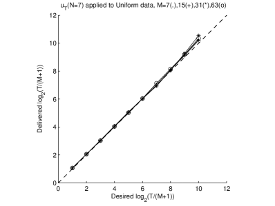
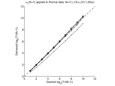
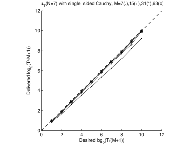
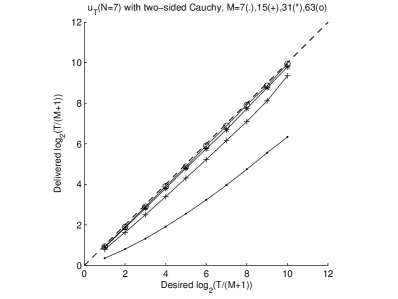
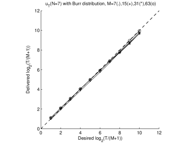
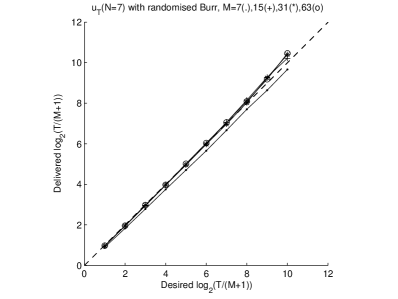
In all cases, as $M$ becomes significantly larger than $N=7$, the probability is matched to increasingly better degrees of approximation. This accords with the general expectation, since the upper quantiles will approach GPDs as $M\gg N$.

In all cases the location- and scale-parameters were randomised (by picking $(\mu,\sigma)$ from normal distributions) for each of the $100,000(M+1)$ samples drawn. However, given that the predictor guarantees location-scale invariance this should not (and did not) affect the performance.

The uniform (upper left) delivers good probability matching at all $M\geq N$, since the uniforms lie within the GPD class.

The normal (upper right) is the first example outside the GPD class. As may be expected, the predictor based on the $N=7$ upper order statistics delivers poor performance for a sample of size $M=7$ (because the upper 7 data points are the full data set, and these will have a two-sided normal distribution, and are thus blatantly far from the GPD, and are in no sense extreme values). However, the probability matching improves dramatically as the sample size $M$ increases even moderately beyond $N=7$.

For the two Cauchy examples (centre, Fig. 7) the performance is good in the one-sided case for all $M$, but requires higher $M$ in the two-sided case. Again, this follows expectations. It highlights the fact that the problem lies with attempting to extrapolate from non-extreme data, much of which lies below the mode in the two-side case. The good results for the one-sided distribution, even when $M=N$, illustrate that the famously heavy-tails of the Cauchy present little problem.

The results for the Burr distributions (lower figures), taken from the family

$$F(y)=1-(1+y^{A})^{B}\ \ \ \ A,B>0\ \ \ \ \mathrm{with}\ y=\frac{x-\mu}{\sigma}$$ (36)

again illustrate that the predictor works well with heavy-tailed distributions. The lower right figure shows the performance over games played against Burr distributions wherein the parameters $A$ and $B$ (as well as $\mu$ and $\sigma$) are drawn from normal distributions. The good performance obtained when playing against such a large stock of distributions with randomised parameters gives some credence to the claim that $u_{T}$ has properties approaching that of a universal probability-matching extreme value predictor.

Good performance has also been found to be delivered for numerous other distributions, but it should be noted that there are cases where probabilities do not match well. These include Weibull distributions with small shape parameters, and beta distributions where the second parameter is small. “Two population” distributions can also be readily constructed for which the predictor performs poorly. These could be said to be of the “black swan” variety, a simple archetype being 99% uniform over $[0,a]$ with the remaining 1% uniform over $[b,1]$, with $a<<b$. For moderate $N$, most samples contain no information about the existence of the second population above $b$, the unknown unknowns. Extreme predictions are thus mostly based on data from $[0,a]$ whilst next events with high return period are values in $[b,1]$. However, for any extrapolation proposal there will obviously be bad cases, and what is surprising about the proposed predictor is how widely and how often it does work (particularly given how small the sample sizes are for which it does work).

9 Summary

The intuition that a predictor, designed to match probability within the GPD family, might transfer some of its potentially-desirable properties across to more general distributions appears to have been borne out. Although the candidate predictor was only approximately probability-matching across the whole range of GPDs, the precision with which return levels could be delivered, even from small data sets drawn from non-GPD distributions, is remarkable.

Finally, it should be emphasised that it is not the intention of this paper to encourage the extrapolation from three data points to the $T=4096$ level. Rather, suspecting that many current methods of extrapolation are inherently optimistic, the paper has endeavoured to put forward a novel alternative for criticism and/or further development.

Appendix 1: Densities of the normalised data

Let $N$ raw data points $\mathbf{x}=\{x_{1},\ldots,x_{N}\}$ be sampled from a GPD with distribution function

$$F(x\ |\ \mu,\sigma,\xi)=1-{\left(1+\xi\frac{(x-\mu)}{\sigma}\right)}^{-1/\xi}$$ (37)

and density

$$p(x\ |\ \mu,\sigma,\xi)=\frac{1}{\sigma}{\left(1+\xi\frac{(x-\mu)}{\sigma}\right)}^{-1-{1/\xi}}$$ (38)

These functions exist over the appropriate domains $x>\mu$ for $\xi>0$ and $\mu<x<\mu-\sigma/\xi$ for $\xi<0$. The case of $\xi=0$ reduces to the exponential case.

The parameters $(\mu,\sigma,\xi)$ are assumed unknown, and we consider first the case $\xi>0$, defining $\alpha=1/\xi$. This corresponds to the heavy-tailed case.

We define the ordered data $\mathbf{X}=\mathrm{sort}(\mathbf{x})$, such that $X_{1}\leq X_{2}\leq\ldots\leq X_{N}$.

All possible samples of raw data $\mathbf{x}$ form an N-dimensional data space. The possible sorted data samples cover only a semi-infinite prism-shaped subset of a similar N-dimensional space. The density over that prism of the ordered data space is identical to that over an equivalent region of the unordered data space multiplied by a factor $N!$, this being the number of such prisms required to make up the full space.

The density over the prism-shaped space of ordered data is thus

$$p(\mathbf{X}\ |\ \mu,\sigma,\xi)=N!p(\mathbf{x}\ |\ \mu,\sigma,\xi)$$ (39)

Although the parameters are unknown, we may define

$$y_{j}=1+\xi\frac{(X_{j}-\mu)}{\sigma}\qquad\ \ j=1,\ldots N$$ (40)

It follows that $1\leq y_{1}\leq y_{2}\ldots\leq y_{N}$ and over the domain of the $y$’s, their density is

$$p(\mathbf{y}|\alpha)=\frac{N!\alpha^{N}}{(y_{1}y_{2}\ldots y_{N})^{1+\alpha}}$$ (41)

We define $(N-2)$ location- and scale-independent statistics $\mathbf{t}$ via

$$t_{j}\equiv\frac{X_{j+1}-X_{1}}{X_{N}-X_{1}}\qquad j=1,\ldots(N-2)$$ (42)

This is the normalised data $\mathbf{t}$. It is ordered and lies in the unit interval ( $0\leq t_{1}\leq t_{2}\leq\ldots\leq t_{N-2}\leq 1$). Trivially, we can also measure from the opposite end of the interval, defining $\tau_{j}=1-t_{j}$

We also define

$$q=\frac{y_{N}-y_{1}}{y_{N}}$$ (43)

Writing the left and right end points of the unit interval as $t_{0}=0$, $\tau_{0}=1$ and $t_{N-1}=1$, $\tau_{N-1}=0$ respectively then together the $N$ transformations

$$y_{j}=y_{N}(1-q\tau_{j})\ \ \ \mathrm{for}\ j=0,\ldots,(N-1)$$ (44)

have Jacobian $y_{1}^{N-1}q^{N-2}$ and the density in the new variables is

$$p(y_{N},q,\bm{\tau}|\alpha)=\frac{N!\alpha^{N-1}y_{N}^{-N\alpha-1}q^{N-2}}{\prod_{j=0}^{N-2}(1-\tau_{j}q)^{1+\alpha}}$$ (45)

For $q$ fixed, the variable $y_{N}$ is bounded below at $1/(1-q)$. It is removed by integration, using

$$\int_{(1-q)^{-1}}^{\infty}y_{N}^{-N\alpha-1}\ dy_{N}=\frac{(1-q)^{N\alpha}}{N\alpha}$$ (46)

before removal of $q$ via the integration

$$p(\bm{t}|\alpha)=(N-1)!\ \alpha^{N-1}\int_{0}^{1}q^{N-2}(1-q)^{(N-1)\alpha-1}\prod_{j=1}^{N-2}(1-\tau_{j}q)^{-(1+\alpha)}\ dq$$ (47)

This is a standard Euler integral representation of a Lauricella function $F_{D}^{(N-2)}$ (Exton, 1978) leading to the desired density

$$p(\bm{t}|\alpha)=N_{1}!\ \alpha^{N_{1}}\ \Gamma\left[\begin{array}[]{c}N_{1},\ N_{1}\alpha\\ N_{1}(1+\alpha)\end{array}\right]F_{D}^{(N-2)}\left(N_{1},\bm{1}+\bm{\alpha};N_{1}(1+\alpha);\bm{\tau}\right)$$ (48)

where $N_{1}=N-1$, and $\bm{1}+\bm{\alpha}$ is a vector of length $N-2$ with each element being $1+\alpha$.

The Lauricella function may be expressed using one of its Euler transformations (Exton, 1976) to give the alternative expression

$$p(\bm{t}|\alpha)=N_{1}!\ \alpha^{N_{1}}\ \Gamma\left[\begin{array}[]{c}N_{1},\ N_{1}\alpha\\ N_{1}(1+\alpha)\end{array}\right]\frac{t_{1}^{(N-2)\alpha-1}}{(t_{2}\ldots t_{N-2})^{1+\alpha}}F_{D}^{(N-2)}\left(N_{1}\alpha,\bm{1}+\bm{\alpha};N_{1}(1+\alpha);\bm{\kappa}\right)$$ (49)

where

$$\kappa_{1}=1-t_{1},\ \ \qquad\kappa_{j}=1-\frac{t_{1}}{t_{j}}\ \ \ \mathrm{for}\ j=2,\ldots N-2$$ (50)

The advantage of this representation is that for sufficiently small $\alpha$, the leading Lauricella parameter $(N-1)\alpha$ is small such that the Lauricella function is close to unity.

For the bounded-tail case, we define $\beta\equiv-1/\xi$ with $\beta>0$, and a similar derivation leads to

$$p(\bm{t}|\beta)=N_{1}!\ \beta^{N_{1}}\ \Gamma\left[\begin{array}[]{c}N_{1},\ \beta\\ N_{1}+\beta\end{array}\right]F_{D}^{(N-2)}\left(N_{1},\bm{1}-\bm{\beta};N_{1}+\beta;\bm{t}\right)$$ (51)

where $\bm{\beta}=\beta\bm{1}$. It should be noted that this is not simply the $\xi>0$ expression with the substitution $\alpha\rightarrow-\beta$ since the bounded nature of the tails leads to different limits in the various integrations.

Appendix 2. Derivation of $G(s_{T}(\bm{t})|\xi)p(\bm{t}|\xi)$

The integral

$$\int_{\forall\bm{t}}\ G(s_{T}(\bm{t})|\xi)\ p(\bm{t}|\xi)\ d\bm{t}$$ (52)

is the (average) probability performance delivered at some given tail parameter $\xi$ by any (normalised) predictor $s_{T}(\bm{t})$ which is a function of the (normalised) data $\bm{t}$. The rest of this paper concerns itself with attempting to construct such a function $s_{T}(\bm{t})$ such that the integral 52 is independent of $\xi$.

The functional form of the integrand $G(s_{T}(\bm{t})|\xi)p(\bm{t}|\xi)$ can be derived from first principles in a manner akin to the derivations of Appendix 1 or, equivalently, via appropriate integration of the Appendix 1 results, as here.

Consider an ordered sample of size $(N+1)$ drawn from a GPD with shape parameter $\xi$. Let the normalised data be $\mathbf{h}=\{h_{1},\ldots h_{N-1}\}$. This normalised data is related to the normalised data $\bm{t}$ plus an extra normalised data point $s$ via $h_{j}=t_{j}/s$ for $j=1$ to $N-1$.

For $\xi>0$ ($\xi=1/\alpha$), the density of $\mathbf{h}$ is obtained from Eqn. (48) as

$$p(\mathbf{h}|\alpha)=\frac{N!}{N+1}\ \alpha^{N}\ \Gamma\left[\begin{array}[]{c}N,\ N\alpha\\ N(1+\alpha)\end{array}\right]F_{D}^{(N-1)}\left(N,\bm{1}+\bm{\alpha};N(1+\alpha);\bm{1}-\mathbf{h}\right)$$ (53)

The $N+1$ divisor must be introduced since we are considering only that $1/(N+1)$ fraction of cases where the next data point $x_{N+1}$ exceeds the historical data maximum.

Substituting $h_{j}=t_{j}/s$ (a transformation with Jacobian $1/s^{N}$) leads to the joint density for $\bm{t}$ and $s>1$ of

$$p(s,\bm{t}|\alpha)=\frac{N!}{N+1}\ \alpha^{N}\ \Gamma\left[\begin{array}[]{c}N,\ N\alpha\\ N(1+\alpha)\end{array}\right]\frac{1}{s^{N}}F_{D}^{(N-1)}\left(N,\bm{1}+\bm{\alpha};N(1+\alpha);\bm{1}-\frac{\bm{t}}{s}\right)$$ (54)

where the vectors extend from $j=1$ to $N-1$.

Using one of the standard Lauricella transforms (Exton, 1976) this can be written

$$p(s,\bm{t}|\alpha)=\frac{N!}{N+1}\ \alpha^{N}\ \Gamma\left[\begin{array}[]{c}N,\ N\alpha\\ N(1+\alpha)\end{array}\right]F_{D}^{(N-1)}\left(N,\bm{1}+\bm{\alpha};N(1+\alpha);1-s,1-\bm{t}\right)$$ (55)

This now needs to be integrated from $s=s_{T}$ to $\infty$ to obtain the tail probability.

It follows from the Euler integral representation of the Lauricella function that

$$\int_{s_{T}}^{\infty}\ F_{D}^{(n)}(a,b_{1},\ldots,b_{n};c;1-s,x_{2},\ldots,x_{n})\ ds\hskip 113.81102pt$$

$$=\frac{(c-1)}{(b_{1}-1)(a-1)}F_{D}^{(n)}(a-1,b_{1}-1,b_{2},\ldots,b_{n};c-1;1-s_{T},x_{2},\ldots,x_{n})$$ (56)

This leads to

$$G(s_{T}(\bm{t})|\alpha)p(\bm{t}|\alpha) = \int_{s_{T}}^{\infty}\ p(s,\bm{t}|\alpha)\ ds$$ (57)

$$= \frac{N!}{N+1}\ \alpha^{N-1}\ \Gamma\left[\begin{array}[]{c}N-1,\ N\alpha\\ N+N\alpha-1\end{array}\right]\ldots$$ (61)

$$\times\ F_{D}^{(N-1)}\left(N-1,\alpha,\bm{1}+\bm{\alpha};N+N\alpha-1;1-s,1-\bm{t}\right)$$

A further Lauricella transform leads to the final form

$$G(s_{T}(\bm{t})|\alpha)p(\bm{t}|\alpha) = \frac{N!}{N+1}\ \alpha^{N-1}\ \Gamma\left[\begin{array}[]{c}N-1,\ N\alpha\\ N+N\alpha-1\end{array}\right]\frac{t_{1}^{(N-1)\alpha-1}}{(t_{2}\ldots t_{N-2})^{1+\alpha}}\frac{1}{s^{\alpha}}\ldots$$ (65)

$$\times F_{D}^{(N-1)}\left(N\alpha,\bm{1}+\bm{\alpha},\alpha;N+N\alpha-1;\mathbf{r}\right)$$

with $r_{j}=1-t_{1}/t_{j}$ for $j=2$ to $N$ (where $t_{N-1}=1$ and $t_{N}=s_{T}$) .

A similar derivation, omitted for brevity, for the bounded-tail case with $\xi$ negative ($\beta=-1/\xi$ positive), leads to

$$G(s_{T}(\bm{t})|\beta)p(\bm{t}|\beta) = \frac{N!}{N+1}\ \beta^{N_{1}}\ \Gamma\left[\begin{array}[]{c}N_{1},\ 1+\beta\\ N+\beta\end{array}\right]\ldots$$ (69)

$$\times\frac{1}{s_{T}^{N_{1}}}F_{D}^{(N_{1})}\left(N_{1},\bm{1}-\bm{\beta};N+\beta;\frac{\bm{t}}{s_{T}}\right)$$

where $\bm{t}=\{t_{j}\}$ for $j=1$ to $N_{1}=N-1$ (with $t_{N-1}=1$). Again, this is not simply the $\xi>0$ expression with $\alpha\rightarrow-\beta$, owing to the bounded nature of the tails changing various integration limits.

Eqns. 65 and 69 for the exceedance probability of the predictor play a central role in the main paper. For $s_{T}(\bm{t})$ to be a probability-matching predictor, the integral of $G(s_{T}(\bm{t})|\xi)p(\bm{t}|\xi)$ over all possible data $\bm{t}$ should equal the desired exceedance probability $1/T$, and this should be true at any value of the tail parameter $\xi$.

Appendix 3: The constraint on the power law exponents in the bounded-tail case

We derive forms for power law predictors for the extreme bounded-tail case (where $\xi=-1/\beta$ and $\beta$ is small and positive).

In the $\xi>0$ case, a constraint on the power-law exponents was derived directly from the small $\alpha$ behaviour of the Lauricella form of $G(s_{T}(\bm{t})|\alpha)p(\bm{t}|\alpha)$ of Eqn. 16. Unfortunately, a similar procedure does not seem possible via $G(s_{T}(\bm{t})|\beta)p(\bm{t}|\beta)$ of Eqn. 20 (or any of its Lauricella transformations or asymptotic forms) in the bounded-tail case. Instead, it is necessary to return to first principles, inserting the small $\beta$ approximation en route.

For a sample of size $N$ drawn from a GPD in the bounded-tail case, the density of the ordered, normalised data $\bm{t}$ is given by a Lauricella transformation of Eqn. LABEL:Frechdens as

$$p(\bm{t}|\beta)\ d\bm{t} = N_{1}!\ \beta^{N_{1}}\ \Gamma\left[\begin{array}[]{c}N_{1},\ \beta\\ N_{1}+\beta\end{array}\right]\frac{\tau_{N-2}^{2\beta-1}}{(\tau_{1}\ldots\tau_{N-3})^{1-\beta}}$$ (73)

$$\hskip 28.45274pt\times\ F_{D}^{(N-2)}(\beta,N_{1}\beta+1,1-\bm{\beta};N_{1}+\beta;\bm{\Psi})\ d\bm{t}$$

with $N_{1}=N-1$, $\bm{\tau}=1-\bm{t}$, and $\psi_{j}=1-\tau_{N-2}/\tau_{j}$ for $j=0$ to $N-3$ (where $\tau_{0}=1$).

Consider now drawing an additional data point $x_{N+1}$. This might not exceed the sample maximum, but we restrict attention to the $1/(N+1)$ fraction of cases when it does. The density of the ordered, normalised data $\bm{t^{\dagger}}$ in this region is thus given by Eqn. 73, with $N\rightarrow N+1$ and $\bm{t}\rightarrow\bm{t}^{\dagger}=[\bm{t}/s_{*},1/s_{*}]$. That is,

$$p({\bm{t}}^{\dagger}|\beta)\ d\bm{t}^{\dagger} = \frac{N!}{N+1}\ \beta^{N}\ \Gamma\left[\begin{array}[]{c}N,\ \beta\\ N+\beta\end{array}\right]\frac{(\tau_{N-1}^{\dagger})^{2\beta-1}}{(\tau_{1}^{\dagger}\ldots\tau_{N-2}^{\dagger})^{1-\beta}}$$ (77)

$$\hskip 28.45274pt\times\ F_{D}^{(N-1)}(\beta,N\beta+1,1-\bm{\beta};N+\beta;\bm{\Psi}^{\dagger})\ d\bm{t}^{\dagger}$$

where

$$\tau_{j}^{\dagger}=1-t_{j}^{\dagger}=1-t_{j}/s_{*}=\frac{u_{*}+\tau_{j}}{1+u_{*}}\ \ \mathrm{and}\ \psi_{j}^{\dagger}=1-\frac{\tau_{N-1}^{\dagger}}{\tau_{j}^{\dagger}}=\frac{\tau_{j}}{u_{*}+\tau_{j}}$$ (78)

with $u_{*}=s_{*}-1$. The leading $N+1$ in the denominator of Eqn 77 accounts for the fact we only consider those cases where the next data point exceeds the sample maximum.

The Jacobian of the transformation gives

$$d\bm{t}^{\dagger}=\frac{1}{s_{*}^{N}}d\bm{t}ds_{*}=\frac{1}{(1+u_{*})^{N}}d\bm{\tau}du_{*}$$ (79)

leading to

$$p(\bm{\tau},u_{*}|\beta)\ d\bm{\tau}du_{*}\ =\ \frac{N!}{N+1}\ \beta^{N}\ \Gamma\left[\begin{array}[]{c}N,\ \beta\\ N+\beta\end{array}\right]\frac{u_{*}^{2\beta-1}}{(1+u_{*})^{N\beta+1}\prod_{j=1}^{N-2}(u_{*}+\tau_{j})^{1-\beta}}$$ (82)

$$\hskip 28.45274pt\times\ F_{D}^{(N-1)}(\beta,N\beta+1,1-\bm{\beta};N+\beta;\frac{1}{1+u_{*}},\frac{\bm{\tau}}{u_{*}+\bm{\tau}})\ d\bm{\tau}du_{*}$$ (83)

We know that

$$d\bm{\tau}\int_{u(\bm{\tau})}^{\infty}\ p(\bm{\tau},u_{*}|\beta)du_{*}=G(u(\bm{\tau})|\beta)p(\bm{\tau}|\beta)d\bm{\tau}\$$ (84)

and already have an exact expression for this (Eqn 69). However, it has not yet been possible to deduce a predictor, not even an approximate one, from that expression. Instead we need to pursue a more circuitous route.

Rather than considering the tail integral directly (i.e. $G(u(\bm{\tau})|\xi)p(\bm{\tau}|\xi)$), we endeavour to approximate instead the integral over the region between the data maximum and the prediction, viz:

$$\int_{\forall\bm{\tau}}\ \int_{0}^{u}\ p(\bm{\tau},u_{*})\ du_{*}\ d\bm{\tau}=\frac{1}{N+1}-\frac{1}{T}$$ (85)

leading to

$$1-\frac{N+1}{T}=N!\beta^{N}\Gamma\left[\begin{array}[]{c}N,\ \beta\\ N+\beta\end{array}\right]\int_{\forall\bm{\tau}}\ \int_{0}^{u}\frac{u_{*}^{2\beta-1}}{(1+u_{*})^{N\beta+1}\prod_{j=1}^{N-2}(u_{*}+\tau_{j})^{1-\beta}}$$ (88)

$$\hskip 28.45274pt\times\ F_{D}^{(N-1)}(\beta,N\beta+1,1-\bm{\beta};N+\beta;\frac{1}{1+u_{*}},\frac{\bm{\tau}}{u_{*}+\bm{\tau}})\ du_{*}d\bm{\tau}$$ (89)

This expression is exact, and if a function $u(\tau)$ could be found which satisfies this then we would have our exact probability matching predictor for all $\beta>0$. This has not yet been possible, and thus we proceed with an approximation.

At the first level of approximation, we could set $F_{D}^{(N-1)}(\beta,\ldots)\approx 1$ and for $u\ll\tau_{j}$ we could ignore the $u_{*}$ terms in the denominator. Postulating a power law predictor of the form $u=\prod_{j}\tau_{j}^{\rho_{j}}$ then leads to a constraint equation for the exponents $\rho_{j}$. However, the resulting predictor has very limited validity: it applies at $N=3$, but for higher $N$ it is valid only for very small extrapolations beyond the data. We thus proceed directly to an improved approximation.

Assuming $F_{D}^{(N-1)}(\beta,\ldots)\approx 1$, and writing $u_{*}=wu$ the inner integral becomes (for $u\ll 1$)

$$I_{u} = \int_{0}^{u}\ \frac{u_{*}^{2\beta-1}}{(1+u_{*})^{N\beta+1}\prod_{j=1}^{N-2}(u_{*}+\tau_{j})^{1-\beta}}\ du_{*}$$

$$= u^{2\beta-1}\prod_{j=1}^{N-2}\tau_{j}^{\beta-1}.\int_{0}^{u}w^{2\beta-1}\left[\prod_{j=1}^{N-2}\left(1+\frac{u}{\tau_{j}}w\right)^{\beta-1}\right]\ (1+uw)^{-N\beta-1}\ udw$$

$$= u^{2\beta}\prod_{j=1}^{N-2}\tau_{j}^{\beta-1}\Gamma\left[\begin{array}[]{c}2\beta,\ 1\\ 1+2\beta\end{array}\right]F_{D}^{(N-1)}(2\beta,1+N\beta,1-\bm{\beta};1+2\beta;-u,\frac{-u}{\bm{\tau}})$$ (93)

For small $\beta$, the gamma function approaches $1/2\beta$.

The Lauricella function can be transformed on its argument of largest magnitude $-u/\tau_{N-2}\equiv x_{1}$ using Exton (1976) (Eqn. 4.2.4, second transformation). The new arguments are

$$\frac{x_{1}}{x_{1}-1}=\frac{u}{u+\tau_{N-2}}\ \ \mathrm{and}\ \ \frac{x_{1}-x_{j}}{x_{1}-1}=\left(\frac{u}{u+\tau_{N-2}}\right)\left(1-\frac{\tau_{N-2}}{\tau_{j}}\right)$$ (94)

These are of interest only in that they are less than unity, and thus the transformed Lauricella function $F_{D}^{(N-1)}(2\beta,\ldots)$ can be approximated as unity for $\beta$ small. This only leaves the leading factor in the Lauricella transformation

$$(1-x_{1})^{-a}=\left(1+\frac{u}{\tau_{N-2}}\right)^{-2\beta}$$ (95)

and we thus obtain

$$I_{u}\approx\frac{1}{2\beta}\left(\frac{u}{u+\tau_{N-2}}\right)^{2\beta}\ \tau_{N-2}^{2\beta}\ \prod_{j=1}^{N-2}\tau_{j}^{\beta-1}$$ (96)

Now, assume a power-law predictor such that

$$\frac{u}{u+\tau_{N-2}}=\prod_{j=1}^{N-2}\tau_{j}^{\rho_{j}}\ \ \mathrm{for}\ \mathrm{some}\ \rho_{j}$$ (97)

To match probability in the extreme bounded-tail limit $\xi\rightarrow-\infty$ we require

$$1-\frac{N+1}{T}=\frac{N!}{2}\ \beta^{N-2}\int_{\forall\bm{\tau}}\ \tau_{N-2}\prod_{j=1}^{N-2}\tau_{j}^{\beta(2\rho_{j}+1)-1}\ d\bm{\tau}$$ (98)

(where we have approximated the two gamma functions by $1/\beta$ and $1/2\beta$ as appropriate for $\beta$ small).

The domain of integration is $\int_{0}^{1}d\tau_{1}\int_{0}^{\tau_{1}}d\tau_{2}\ldots\int_{0}^{\tau_{N-3}}d\tau_{N-2}$, leading to

$$1-\frac{N+1}{T} = \frac{N!\beta^{N-2}}{2.(2\rho_{N-2}+3)\beta\ldots(2(\rho_{N-2}+\ldots+\rho_{1})+N)\beta}$$ (99)

$$= \frac{N!}{2}\prod_{k=1}^{N-2}\left(2\eta_{k}+(k+2)\right)^{-1}$$ (100)

That is, our predictor $u(\bm{\tau})$ is

$$u=\tau_{N-2}\ \frac{\prod_{j=1}^{N-2}\tau_{j}^{\rho_{j}}}{1-\prod_{j=1}^{N-2}\tau_{j}^{\rho_{j}}}\equiv u_{\beta}$$ (101)

where the exponents satisfy

$$\prod_{k=1}^{N-2}\left[\frac{2\eta_{k}}{k+2}+1\right]=\frac{1}{1-\frac{N+1}{T}}$$ (102)

with partial sums

$$\eta_{k}=\sum_{i=N-1-k}^{N-2}\rho_{i}$$ (103)

The above derivation suggests that this should give the correct exceedance probability $1/T$ in the extreme bound-tail limit of GPDs with $\xi$ large and negative, and the numerical results presented in the main text (Fig. 2) suggest that it does.

References

- Coles and Tawn (2005) Coles, S., Tawn, J., 2005. Bayesian modelling of extreme surges on the UK east coast. Phil. Trans. R. Soc. A 363, 1387–1406.
- Datta and Mukerjee (2004) Datta, G. S., Mukerjee, R., 2004. Probability Matching Priors: Higher Order Asymptotics. Lecture Notes in Statistics. Springer, New York.
- Embrechts et al. (1999) Embrechts, P., Klüppelberg, C., Mikosch, T., 1999. Modelling Extreme Events for Insurance and Finance. Springer, Berlin.
- Exton (1976) Exton, H., 1976. Multiple Hypergeometric Functions and Applications. Ellis Horwood, Chichester, UK.
- Exton (1978) Exton, H., 1978. Handbook of Hypergeometric Integrals. Ellis Horwood, Chichester, UK.
- McRobie (2004) McRobie, F. A., 2004. Exact exceedance estimators and the reference prior. Tech. Rep. CUED/D-STRUCT/TR213, Cambridge University Engineering Dept.
- McRobie (2013a) McRobie, F. A., 2013a. Elemental estimators for the Generalized Extreme Value tail. arxiv:1304.4362.
- McRobie (2013b) McRobie, F. A., 2013b. Elemental unbiased estimators for the Generalized Pareto tail. arxiv:1304.3918.
- Sweeting (2008) Sweeting, T., 2008. On predictive probability matching priors. In: Clarke, B., Ghosal, S. (Eds.), IMS Collections: Pushing the Limits of Contemporary Statistics: Contributions in Honor of Jayanta K. Ghosh. No. 3. pp. 46–59.